Expansion of a mesoscopic Fermi system from a harmonic trap

Abstract

We study quantum dynamics of an atomic Fermi system with a finite number of particles, $N$, after it is released from a harmonic trapping potential. We consider two different initial states: The Fermi sea state and the paired state described by the projection of the grand-canonical BCS wave function to the subspace with a fixed number of particles. In the former case, we derive exact and simple analytic expressions for the dynamics of particle density and density-density correlation functions, taking into account the level quantization and possible anisotropy of the trap. In the latter case of a paired state, we obtain analytic expressions for the density and its correlators in the leading order with respect to the ratio of the trap frequency and the superconducting gap (the ratio assumed small). We discuss several dynamic features, such as time evolution of the peak due to pair correlations, which may be used to distinguish between the Fermi sea and the paired state.

Introduction — Measurements of density distributions and noise correlations in time-of-flight expansion have proven to be a very powerful direct probe of the quantum states of cold atomic systems. In bosonic systems, density distributions contain valuable information about the initial quantum state and allow one to observe directly Bose-Einstein condensates. In cold Fermi systems, the time-of-flight density profile of a Fermi liquid is expected to be qualitatively similar to the one of a paired state. Altman et al. Altman et al. (2004) have shown that to identify the existence of a BCS condensate, one should probe noise correlations, which in the condensed state would acquire a peak at the opposite momenta corresponding to Cooper pairing. Greiner et al. Greiner et al. (2005) have experimentally observed similar pairing correlations of fermionic atoms on the BEC side of a Feshbach resonance, showing the experimental feasibility of the proposed method. However, so far there have been no direct observations of pairing correlations in the BCS state, which was detected in Ref. [Schunck et al., ] by different means.

Most previous theoretical studies have concentrated on the dynamic properties of density and its correlators, which followed from the grand canonical wave-functions. However, all real experimentally studied systems are finite and non-uniform due to the trapping potential. Moreover, the grand canonical description is strictly speaking not appropriate in this context, since non-trivial density fluctuations may exist only if the system is finite and formally vanish in thermodynamic limit. It is therefore important to consider expansion dynamics of a finite system in a realistic trapping potential. We should mention here that there exist a number of exact results for a Fermi system in a harmonic potential: See e.g., Ref. [Schneider and Wallis, 1998], which considered thermodynamic properties of a mesoscopic Fermi gas and Refs. [Brack and Murthy, 2003; Wang, 2002; Gleisberg et al., 2000; B. P. van Zyl et al., 2003; Bruun, 2001] where density and energy distributions were studied. Also, Bruun and Heiselberg Bruun and Heiselberg (2002) investigated the properties of a paired state of trapped fermions.

In this work we extend these studies to the dynamic regime of an expanding Fermi cloud. We explicitly calculate density distributions and noise correlations using the canonical formulation and taking into account discrete energy levels and a finite number of particles in a harmonic trap. In the case of a Fermi sea state, we derive exact and simple analytic expressions for the density and its correlators. To describe a paired state, we use the grand canonical BCS wave-function projected onto the subspace with a fixed number of particles - projected BCS (PBCS) state. This wave-function was written explicitly in the original paper of Bardeen, Cooper, and Shrieffer Bardeen et al. (1957) and then used in the context of nanoscale superconductors von Delft (2001). We should mention here that there exists an exact solution of the reduced BCS Hamiltonian due to Richardson Richardson (1963); Richardson and Sherman (1964), who found a set of equations, which determine the energy levels in a finite Fermi system with attractive interactions and constructed an exact wave-function in this case. However, to use this exact solution is difficult due to the complicated structure of the Richardson’s equations. Moreover, it has been shown von Delft (2001) that the exact Richardson’s wave function reduces to the PBCS state if the superconducting gap $\Delta$ is much larger than the level spacing (in fact the BCS Ansatz remains a good approximation even if the ratio of the gap and level spacing is of order unity Braun and von Delft (1999); von Delft (2001)). Below, we consider the latter limit, which in the context of a trapped Fermi gas corresponds to $\Delta\gg\omega$, where $\omega$ is the frequency of the trapping potential.

Time-dependent density — Let us consider a Fermi system in a harmonic trap in a quantum many-body state $|\Phi\rangle$. We are interested in the dynamics of density and its correlators after the harmonic potential and interactions, if present, are turned off at $t=0$. For simplicity, we start with the one-dimensional case. We will see that generalization of all results to higher dimensions is straightforward. The time-dependent density is

$$\langle n(x,t)\rangle=\langle\Phi|\hat{U}_{0}^{+}(t)\hat{\psi}^{+}(x)\hat{\psi}(x)\hat{U}_{0}(t)|\Phi\rangle,$$ (1)

where $\hat{U}_{0}(t)=\exp\left(-i\sum_{p}E_{p}\hat{a}^{+}_{p}\hat{a}_{p}\,t\right)$ is the evolution operator of the free system, $E_{p}=p^{2}/(2m)$, and $\hat{\psi}(x)=\sum_{n}\psi_{n}(x)\hat{a}_{n}$ is the field operator, where $\psi_{n}(x)$ and $\hat{a}_{n}$ are the oscillator wave-function and the annihilation operator in the harmonic potential corresponding to the $n$-th level. Introducing the Fourier transform of the oscillator wave-functions $\tilde{\psi}_{n}(p)$, we can write the density in the following form

$$\langle n(x,t)\rangle=\sum_{n,m}\int\frac{dq}{2\pi}\,\frac{dP}{2\pi}\,e^{iq\left(x-i\frac{P}{m}t\right)}\tilde{\psi}^{*}_{n}\left(P+\frac{q}{2}\right)\tilde{\psi}_{m}\left(P-\frac{q}{2}\right)\langle\hat{a}^{+}_{n}\hat{a}_{m}\rangle.$$ (2)

We note that if we neglect the $q$-dependence of the wave functions (which is a good approximation if $t\gg\omega^{-1}$), we recover the “natural” result for the density Altman et al. (2004)

$$\langle n\rangle\approx\sum_{n,m}\tilde{\psi}^{*}_{n}(P)\tilde{\psi}_{m}(P)\langle a^{+}_{n}a_{m}\rangle\Bigr{|}_{P=mx/t}.$$

We also note that Eq. (2) is exact and valid for any many-body state $|\Phi\rangle$, assuming that interactions are absent at $t>0$.

Fermi gas — Now let us consider a Fermi sea state at zero temperature, which means that $|\Phi\rangle=\prod\limits_{n=0}^{N-1}\hat{a}^{\dagger}_{n}|{\rm vac}\rangle$. We find

$$\langle n(x,t)\rangle=\sum\limits_{n=0}^{N-1}\frac{2\pi}{2^{n}n!\sqrt{\pi}m\omega}\int\,\frac{dp}{2\pi}\,\frac{dp^{\prime}}{2\pi}\,H_{n}\left(\frac{p}{\sqrt{m\omega}}\right)H_{n}\left(\frac{p^{\prime}}{\sqrt{m\omega}}\right)\\ \times e^{i(p-p^{\prime})x}e^{i(E_{p^{\prime}}-E_{p})(t+\frac{i}{\omega})}.$$ (3)

The integrals over $p$ and $p^{\prime}$ are table integrals and we obtain

$$\langle n(x,t)\rangle=\sum\limits_{n=0}^{N-1}\psi_{n}^{2}\left[x,\omega(t)\right],$$ (4)

where $\psi_{n}\left[x,\omega(t)\right]$ is the oscillator wave function with a “rescaled” frequency $\omega(t)=\omega/(1+\omega^{2}t^{2}).$ The sum in Eq. (4) can be calculated exactly and we find

$$\langle n(x,t)\rangle=\frac{e^{-x^{2}/\xi^{2}}}{2^{N}(N-1)!\sqrt{\pi}\xi}\left[H^{2}_{N}\left(\frac{x}{\xi}\right)-H_{N+1}\left(\frac{x}{\xi}\right)H_{N-1}\left(\frac{x}{\xi}\right)\right],$$ (5)

where we introduced $\xi={\sqrt{1+\omega^{2}t^{2}}}/{\sqrt{m\omega}}$. We see that the behavior of the density is determined by the wave-functions near the “Fermi level” $n_{\rm F}=N-1$. One can also check by explicit calculation that the integral over $x$ of Eq. (5) naturally reproduces the total number of particles in the system. It is also easy to generalize the result (4) to the three-dimensional case. In the case of an anisotropic trap with frequencies $\omega_{x,y,z}$ in the corresponding directions, we find

$$\langle n({\bf r},t)\rangle=\sum\limits_{E_{n_{x},n_{y},n_{z}}<E_{\rm F}}\psi_{n_{x}}^{2}\left[x,\omega_{x}(t)\right]\psi_{n_{y}}^{2}\left[y,\omega_{y}(t)\right]\psi_{n_{z}}^{2}\left[z,\omega_{z}(t)\right],$$ (6)

where $E_{\rm F}$ is the Fermi level, $E_{n_{x},n_{y},n_{z}}=\omega\left(n_{x}+n_{y}+n_{z}+3/2\right)$, and $\omega_{\alpha}(t)=\omega_{\alpha}/(1+\omega_{\alpha}^{2}t^{2})$. This result (6) allows us to determine the dynamic ratio of the radii of the time-dependent density distribution. E.g., let us assume that $\omega_{x}=\omega_{y}=\omega_{\perp}>\omega_{z}$. The dynamic aspect ratio is determined by the ratio of the spreads of the wave-functions corresponding to the fermions occupying the highest possible levels $n_{x,z}^{\rm max}=E_{\rm F}/\omega_{x,z}$.

$$\frac{R_{\perp}(t)}{R_{z}(t)}\sim\frac{\sqrt{n_{x}^{\rm max}}\xi_{\perp}(t)}{\sqrt{n_{z}^{\rm max}}\xi_{z}(t)}=\frac{\omega_{z}}{\omega_{\perp}}\,\frac{\sqrt{1+\omega_{\perp}^{2}t^{2}}}{\sqrt{1+\omega_{z}^{2}t^{2}}}.$$ (7)

We therefore reproduce the classical formula of Ref. [Menotti et al., 2002]. According to Eq. (7), the ratio crosses over from the initial value $\omega_{z}/\omega_{\perp}<1$ at $t=0$ to a final constant value 1 at $t\to\infty$. We mention here that the dynamics of the single particle wave-functions corresponding to low-lying levels of the harmonic potential are different: The ratio of the spreads of the corresponding wave-packets behaves as $\frac{\xi_{\perp}}{\xi_{z}}=\frac{\sqrt{\omega_{z}}}{\sqrt{\omega_{\perp}}}\,\frac{\sqrt{1+\omega_{\perp}^{2}t^{2}}}{\sqrt{1+\omega_{z}^{2}t^{2}}}$ and crosses over from the initial value $\sqrt{\omega_{z}/\omega_{\perp}}<1$ at $t=0$ to a final constant value $\sqrt{\omega_{\perp}/\omega_{z}}>1$ at $t\to\infty$.

In the case of an isotropic three-dimensional trap, we can rewrite Eq. (6) in the form

$$\langle n({\bf r},t)\rangle=\sum\limits_{n<n_{\rm F},l}\,\,\,\,(2l+1)R_{nl}^{2}\left[r,\omega(t)\right],$$ (8)

where $R_{nl}(r,\omega)$ is the radial wave-function of a harmonic potential with a frequency $\omega$, $R_{nl}=C_{nl}e^{-r^{2}/\xi^{2}}(r/\xi)^{l}F\left[-(n-l)/2,l+3/2,-r^{2}/\xi^{2}\right]$ with $F(\cdot)$ being the hypergeometric function.

We also mention here that generalization of the obtained results to the case of a finite temperature is straightforward. Indeed, Eq. (8) describes a superposition of single-particle wave-functions corresponding to the occupied states. At zero temperature all states below the Fermi level are occupied with the equal probability. At finite temperatures, we have to weight each state with the probability determined by the Fermi distribution function $f(E,T)=\left\{1+\exp\left[\frac{E-\mu(T)}{T}\right]\right\}^{-1}$, where $\mu(T)$ can be found from the relation $\sum_{n}g_{n}f(E_{n})=N$ with $g_{n}=(n+1)(n+2)/2$ being the degeneracy of the $n$-th level. Thus, it is natural to write the finite temperature result as

$$\langle n({\bf r},t;T)\rangle=\sum\limits_{n<n_{\rm F},l}\,\,\,\,(2l+1)R_{nl}^{2}\left[r,\omega(t)\right]f(E_{n},T).$$ (9)

Similarly, one can obtain the density-density noise correlations of a mesoscopic Fermi gas. Below, we just give a finite result of the calculation in the one-dimensional case at $T=0$

$$\langle n(x_{1},t)n(x_{2},t)\rangle=\delta(x_{1}-x_{2})\langle n(x_{1},t)\rangle+\langle n(x_{1},t)\rangle\langle n(x_{2},t)\rangle$$

$$-\frac{e^{-\frac{x_{1}^{2}+x_{2}^{2}}{\xi^{2}}}\left[H_{N-1}\left(\frac{x_{1}}{\xi}\right)H_{N}\left(\frac{x_{2}}{\xi}\right)-H_{N}\left(\frac{x_{1}}{\xi}\right)H_{N-1}\left(\frac{x_{2}}{\xi}\right)\right]^{2}}{\pi(N-1)!^{2}\,2^{2N}(x_{1}-x_{2})^{2}},$$ (10)

where $\langle n(x_{1,2},t)\rangle$ is given by Eq. (5). We note that in thermodynamic limit the density correlations vanish. We also mention that higher-order density correlation functions of a Fermi gas can be obtained analytically and have a structure similar to Eq. (10).

Paired state — Now we consider density dynamics of an expanding finite Fermi system initially in the paired state. If the system were infinite, we could use the grand canonical BCS wave-function. However, the latter is not appropriate in the given context since the grand canonical BCS Ansatz does not conserve the number of particles. A superconducting wave-function with a fixed number of particles was discussed by Bardeen, Cooper, and Schrieffer in their seminal paper Bardeen et al. (1957) and later in great detail by von Delft von Delft (2001) and others in the context of ultrasmall superconducting grains. This issue was also investigated by Richardson Richardson (1963); Richardson and Sherman (1964) who found an exact many body wave function of the reduced Hamiltonian

$$\hat{H}=\sum_{nn^{\prime}}\left(\delta_{nn^{\prime}}\varepsilon_{n}\hat{a}_{n\sigma}^{\dagger}\hat{a}_{n^{\prime}\sigma}-\lambda\omega\hat{a}_{n\uparrow}^{\dagger}\hat{a}_{{n_{T}}\downarrow}^{\dagger}\hat{a}_{n^{\prime}\downarrow}\hat{a}_{{n^{\prime}_{T}}\uparrow}\right),$$ (11)

where $|n\rangle$ and $|n_{T}\rangle=\hat{T}|n\rangle$ are pairs of single particle states related to each other by time-reversal, the sum runs over all interacting single-particle levels, and $\varepsilon_{n}$ are the energies of the levels. Model Hamiltonian (11) has been used to describe the properties of nuclei in the nuclear pairing model as well as small superconducting grains with a finite number of particles. The reduced Richardson Hamiltonian should also be an appropriate model to describe a mesoscopic paired Fermi system in a trap, with $n$ corresponding to the quantum levels of the harmonic trap. Note that in the one-dimensional case, the paired states related to each other by time-reversal are identical $|n\rangle=|n_{T}\rangle$, while in a three-dimensional potential they are $|n,l,m\rangle$ and $|n,l,-m\rangle=\hat{T}|n,l,m\rangle$. The exact wave-function of reduced Hamiltonian (11) is

$$|{\rm RBCS}\rangle_{\rm exact}=C_{N}^{\prime}\prod\limits_{\nu}^{N}\sum_{n}\frac{\hat{b}_{n}^{\dagger}}{2\varepsilon_{n}-E_{\nu}}\,|\mathrm{vac}\rangle,$$

where $\hat{b}_{n}^{\dagger}=\hat{a}_{n\uparrow}^{\dagger}\hat{a}_{{n_{T}}\downarrow}^{\dagger}$ and $E_{\nu}$ are solutions of a system of coupled Richardson’s equations Richardson (1963); Richardson and Sherman (1964); von Delft (2001). The latter can not be solved analytically, but one can show that in the limit of large but finite number of particles and small level spacing the exact wave-function is indistinguishable from the variational BCS wave-function projected to the fixed number of particles. This projected BCS wave-function has the form

$$|{\rm PBCS}\rangle=C_{N}\int\frac{d\phi}{2\pi}e^{-i\phi N}\prod_{n}\left(u_{n}+e^{i\phi}v_{n}\hat{b}_{n}^{\dagger}\right)|\mathrm{vac}\rangle,$$ (12)

where $C_{N}$ is a normalization constant and $v_{n}$ and $u_{n}$ are variational parameters. We now use this PBCS wave-function (12) to calculate the dynamics of the density, which follows after the trap and the BCS interaction are turned off. For simplicity, we study the one-dimensional case [generalization to higher dimensions is formally straightforward; see also Eqs. (6, 8) and the corresponding discussion]. From Eqs. (2) and (12), we obtain after some algebra

$$\langle n(x,t)\rangle=\frac{2\sum\limits_{n=0}^{\infty}f_{n}|\psi_{n}[x,\omega(t)]|^{2}\sum\limits_{\{m\}_{N-1}^{n}}\prod\limits_{m\in{{\{m\}_{N-1}^{n}}}}f_{m}}{\sum\limits_{\{n\}_{N}}\prod\limits_{n\in{\{n\}_{N}}}f_{n}},$$ (13)

where $\{n\}_{N}$ implies all possible sets of $N$ quantum levels, $\{m\}_{N-1}^{n}$ denotes all possible sets of $N-1$ quantum levels except $n$, $f_{n}=v_{n}^{2}/u_{n}^{2}$, and $\psi_{n}[x,\omega(t)]$ is the oscillator wave-function with a rescaled frequency $\omega(t)=\omega/(1+\omega^{2}t^{2})$. In the limit $\omega\ll\Delta$, the sum $\sum\limits_{\{m\}_{N-1}^{n}}\prod\limits_{m\in{{\{m\}_{N-1}^{n}}}}f_{m}$, which runs over all possible $(N-1)$ single-particle levels except $|n\rangle$, does not strongly depend on the particular level, which is eliminated from it. Therefore in Eq. (13), it can be treated as a constant and determined from the self-consistency equation $\int dx\langle n(x,t)\rangle=2N$, which leads to the following result

$$\langle n(x,t)\rangle=2N\frac{\sum\limits_{n=0}^{\infty}f_{n}\psi_{n}^{2}[x,\omega(t)]}{\sum\limits^{\infty}_{n=0}f_{n}}.$$ (14)

We see that in contrast to the case of a Fermi gas, the sum does not have a sharp cut-off at the Fermi level. A smooth cut-off is provided by the factor $f_{n}={v_{n}^{2}}/{u_{n}^{2}}$. E.g., if we assume the following expressions for the variational parameters

$$f_{n}=\frac{1-\frac{\varepsilon_{n}}{\sqrt{\varepsilon_{n}^{2}+\Delta^{2}}}}{1+\frac{\varepsilon_{n}}{\sqrt{\varepsilon_{n}^{2}+\Delta^{2}}}},$$ (15)

the sum will be regularized at large indices $n\gg\Delta/\omega$, as $f_{n}\sim 1/n^{2}$ [we assume here that $\Delta$ is of the order of the bulk superconducting gap, $\Delta\sim N^{1/d}\omega\exp(-1/\lambda)$, where $d$ is the dimensionality]. Note that the only qualitative difference between the time-dependent density profile of an expanding Fermi gas (5) and the BCS state (14) is the absence of oscillatory features in the latter. However, we should note that these Friedel oscillations are also absent if the expanding phase is initially a strongly interacting but unpaired Fermi liquid. Indeed in this case, the initial state is a Fermi sea of Landau quasiparticles, which are not the original fermions. Therefore, if the typical interaction energy (or temperature) is larger or of order $\omega$, the oscillatory features are smeared out. Therefore, the time-dependent density of a Fermi liquid state and a paired state are qualitatively indistinguishable.

To derive the correlation function, we need to calculate the following average $\left\langle{\rm PBCS}\right|\hat{a}^{\dagger}_{k\sigma}\hat{a}_{l\sigma}\hat{a}^{\dagger}_{m\sigma^{\prime}}\hat{a}_{n\sigma^{\prime}}\left|{\rm PBCS}\right\rangle$. We note here that the anomalous pair correlators trivially vanish $\left\langle{\rm PBCS}\right|\hat{a}_{l\sigma}\hat{a}_{n\sigma^{\prime}}\left|{\rm PBCS}\right\rangle=0$, because the operators in the pair correlator do not conserve the number of particles while the PBCS wave-function does so by construction. This however does not imply that the quartic average has no anomalous terms. This is due to the fact that the quartic and higher-order averages can not be decomposed into pairs using Wick’s theorem if the underlying Hamiltonian is interacting. However, the quartic average can be calculated directly using Eq. 12).

At this point, we introduce the following notation

$$\alpha_{n}(x,t)=e^{in\varphi(t)}\psi_{n}\left[x,\omega(t)\right],\,\,\,\mbox{ where }\,\,\tan\varphi(t)=\omega t.$$ (16)

This function differs from the usual oscillator wave-function only by a time-dependant phase-factor. Using this notation, we can write in the limit $\omega\ll\Delta$,

$$\langle n(x_{1})n(x_{2})\rangle=\delta(x_{1}-x_{2})\langle n(x_{1})\rangle+2\frac{Z_{N-1}}{Z_{N}}\left|\sum_{n}\alpha_{n1}\alpha_{n2}f^{1/2}_{n}\right|^{2}+\\ +\frac{Z_{N-2}Z_{N}}{2Z^{2}_{N-1}}\langle n(x_{1})\rangle\langle n(x_{2})\rangle-\frac{2Z_{N-2}}{Z_{N}}\left|\sum_{n}\alpha^{*}_{n1}\alpha_{n2}f_{n}\right|^{2},$$ (17)

where $Z_{N}=\sum\limits_{\{n\}_{N}}\prod\limits_{n\in{\{n\}_{N}}}f_{n}$. The second term in Eq. (17) represents the “anomalous” component of the density, which leads to the anomalous spatial correlations in the large-$t$ asymptotic behavior discussed previously by Altman et al. Altman et al. (2004). Let us study the dynamics of this anomalous correlator in detail

$$\langle n(x_{1},t)n(x_{2},t)\rangle_{\rm anom}=2\frac{Z_{N-1}}{Z_{N}}\left|\sum_{n}\alpha_{n}(x_{1},t)\alpha_{n}(x_{2},t)f^{1/2}_{n}\right|^{2}.$$ (18)

At $t=0$, the phase factor in the function $\alpha_{n}(x,0)$ (16) is equal to zero $\phi(0)=0$. If there were no factor $\sqrt{f_{n}}$ in the sum in Eq. (18), the sum would reduce to $\sum_{n}\psi_{n}(x_{1})\psi_{n}(x_{2})=\delta(x_{1}-x_{2})$, which is a same-point delta-function via the resolution of unity. The factor $\sqrt{f_{n}}$, which contains information about pairing, regularizes the sum at large indices and therefore smears out the delta-function leading to a peak of finite width. This has clear physical explanation: At $t=0$, the system is in the PBCS paired state with fermions $|n,\uparrow\rangle$ and $|n,\downarrow\rangle$ paired up. The considered limit $\omega\ll\Delta$ implies that the size of a Cooper pair (coherence length, $\xi_{\rm CP}\sim v_{\rm F}/\Delta\sim\sqrt{{\omega N}/{m\Delta^{2}}}$) is much smaller than the size of the trapping potential at the Fermi level $\xi\sim\sqrt{{N}/{m\omega}}$. In our model, the coherence length is small $\xi\gg\xi_{\rm CP}$ but finite and this leads to a finite width of the peak in the correlation function.

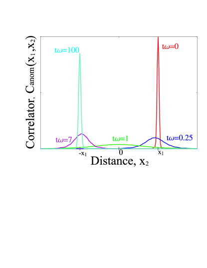
Figure 1: (Color online) The figure shows the anomalous density-density correlator [see Eq. (18)] in rescaled units: $C_{\rm anom}(x_{1},x_{2};t)=\sigma^{2}(t)\left\langle n[x_{1}\sigma(t),t]n[x_{2}\sigma(t),t]\right\rangle$, where $\sigma(t)=\sqrt{1+\omega^{2}t^{2}}$. The correlator is plotted as a function of the coordinate $x_{2}$ with $x_{1}$ fixed. Note that at $t=0$, the correlator is peaked at $x_{2}=x_{1}$, which reflects the fact that the size of a Cooper pair is much smaller than the typical lengthscale determined by the trap. At intermediate times, the correlator shows a smaller peak, which drifts toward the point $x_{2}=-x_{1}$. At large times, the rescaled correlator shows a sharp peak at $x_{2}=-x_{1}$, which corresponds to the initial anti-correlation in momentum space.

At larger times $t>0$, we should consider the sum of type $\sum_{n}\psi_{n}(x_{1})\psi_{n}(x_{2})e^{-in\phi(t)}$, which no longer has the form of a resolution of unity. The behavior of the anomalous correlator (18) was investigated numerically (see Fig 1.) using the Ansatz (15). We note that Fig. 1 shows the evolution of the anomalous peak in terms of rescaled variables as defined in the caption. From Fig. 1, we see that after the expansion $0<\omega t\ll\Delta/\omega$, the initial peak at $x_{1}\sim x_{2}$ becomes smaller and moves toward $x_{1}\sim-x_{2}$. At large times $t\gg\Delta/\omega^{2}$, the peak re-appears exactly at $x_{1}=-x_{2}$ in accordance with Ref. [Altman et al., 2004]. In our formalism, the origin of the peak is due to the fact that the phase factor in Eq. (16) approaches $\phi(t\to\infty)=\pi/2$ at large times. Therefore the sum in the anomalous correlator reduces to $\sum_{n}(-1)^{n}\psi_{n}(x_{1})\psi_{n}(x_{2})\sqrt{f_{n}}$. Using the symmetry properties of the Hermite polynomials, $H_{n}(-x)=(-1)^{n}H_{n}(x)$, one can see that in the absence of the factor $\sqrt{f_{n}}$, the sum reduces to a delta-function $\delta(x_{1}+x_{2})$ at the opposite points. The “BCS factor” $\sqrt{f_{n}}$ smears out the delta-function singularity; again due to a finite size of a Cooper pair in the original condensate.

To summarize, we have derived analytic expressions for the dynamics of particle density and density-density correlation function following a release of a Fermi system from a harmonic trap. We considered two types of initial states: A Fermi gas and a paired BCS state. Our results for the paired state are valid only in the limit of small level spacing $\omega\ll\Delta$. The opposite limit (in which the Cooper pair size is larger than the typical length-scale of the trapping potential) should be similar to the case of an ultra-small superconducting grain (see [von Delft, 2001] and references therein). In the latter case, there is no true superfluidity, but there exist a variety of interesting mesoscopic correlation effects (see, e.g., Ref. [Matveev and Larkin, 1997]), which are in principle accessible in small atomic systems.

Acknowledgements — P.N. was supported by the JQI Graduate Fellowship. The authors are grateful to Carlos Sa de Melo, Vito Scarola, Eite Tiesinga, and Chuanwei Zhang for helpful discussions.

References

- Altman et al. (2004) E. Altman, E. Demler, and M. D. Lukin, Phys. Rev. A 70, 013603 (2004).
- Greiner et al. (2005) M. Greiner, C. A. Regal, J. T. Stewart, and D. S. Jin, Phys. Rev. Lett. 94, 110401 (2005).
- (3) C. H. Schunck, M. W. Zwierlein, A. Schirotzek, and W. Ketterle, cond-mat/0607298 (2006).
- Schneider and Wallis (1998) J. Schneider and H. Wallis, Phys. Rev. A 57, 1253 (1998).
- Brack and Murthy (2003) M. Brack and M. Murthy, J. Phys. A: Math. Gen. 36, 1111 (2003).
- Wang (2002) X.-Z. Wang, J. Phys. A: Math. Gen. 35, 9601 (2002).
- Gleisberg et al. (2000) F. Gleisberg et al., Phys. Rev. A 62, 063602 (2000).
- B. P. van Zyl et al. (2003) B. P. van Zyl, R. K. Bhaduri, A. Suzuki, and M. Brack, Phys. Rev. A 67, 023609 (2003).
- Bruun (2001) G. M. Bruun, Phys. Rev. A 63, 043408 (2001).
- Bruun and Heiselberg (2002) G. M. Bruun and H. Heiselberg, Phys. Rev. A 65, 053407 (2002).
- Bardeen et al. (1957) J. Bardeen, L. N. Cooper, and J. R. Schrieffer, Phys. Rev. 108, 1175 (1957).
- von Delft (2001) J. von Delft, Ann. Phys. (Leipzig) 10, 1 (2001).
- Richardson (1963) R. W. Richardson, Phys. Lett. 3, 227 (1963).
- Richardson and Sherman (1964) R. W. Richardson and N. Sherman, Nucl. Phys. 52, 221 (1964).
- Braun and von Delft (1999) F. Braun and J. von Delft, Phys. Rev. B 59, 9527 (1999).
- Menotti et al. (2002) C. Menotti, P. Pedri, and S. Stringari, Phys. Rev. Lett. 89, 250402 (2002).
- Matveev and Larkin (1997) K. A. Matveev and A. I. Larkin, Phys. Rev. Lett. 78, 3749 (1997).