2cm1cm0.5cm2cm

Hofstadter butterflies of bilayer graphene

Abstract

We calculate the electronic spectrum of bilayer graphene in perpendicular magnetic fields nonperturbatively. To accomodate arbitrary displacements between the two layers, we apply a periodic gauge based on singular flux vortices of phase $2\pi$. The resulting Hofstadter-like butterfly plots show a reduced symmetry, depending on the relative position of the two layers against each other. The split of the zero-energy relativistic Landau level differs by one order of magnitude between Bernal and non-Bernal stacking.

After the theoretical prediction of the peculiar electronic properties of graphene in 1947 by WallaceWallace (1947) and the subsequent studies of its magnetic spectrum,McClure (1956); Zheng and Ando (2002) it took half a century until single layers of graphene could be isolated in experimentNovoselov et al. (2005a) and the novel mesoscopic properties of these two-dimensional (2D) Dirac-like electronic systems, e.g., their anomalous quantum Hall effect, could be measured.Zhang et al. (2005); Novoselov et al. (2005b); Zhang et al. (2006) Inspired by this experimental success, graphene has become the focus of numerous theoretical works.Gusynin and Sharapov (2005); Kane and Mele (2005); Peres et al. (2006); Guinea et al. (2006); Hasegawa and Kohmoto (2006) For bilayers of graphene, an additional degeneracy of the Landau levels and a Berry phase of $2\pi$ were predicted to lead to an anomalous quantum Hall effect, different from either the regular massive electrons or the special Dirac-type electrons of single-layer graphene,McCann and Fal’ko (2006) which was confirmed in experiment shortly afterwardsNovoselov et al. (2006) and used for the characterization of bilayer samples.Ohta et al. (2006)

The low-energy electronic structure of a single layer of graphene is well described by a linearization near the corner points of the hexagonal Brillouin zone ($K$ points), resulting in an effective Hamiltonian formally equivalent to that of massless Dirac particles in two dimensions.DiVincenzo and Mele (1984) A related Hamiltonian can be constructed featuring a supersymmetric structure which can be exploited to derive the electronic spectrum in the presence of an external magnetic field.Ezawa (2006) The level at zero energy, characteristic for any supersymmetric system, maps directly to a special half-filled Landau level fixed at the Fermi energy $E_{\mathrm{F}}$, henceforth called the supersymmetric Landau level (SUSYLL).

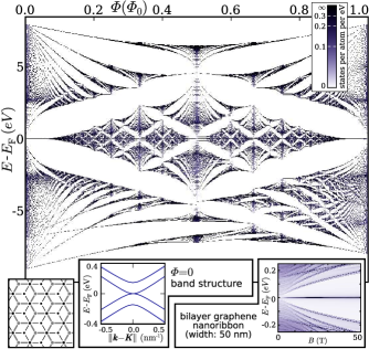
Figure 1: (Color online) Hofstadter butterfly of a bilayer graphene in the Bernal stacking configuration. The band structure at zero magnetic field is rotationally symmetric in good approximation for an area around the $K$ point and shows a split into four massive bands, with the two middle ones touching at $E_{\mathrm{F}}$. The density of states (DOS) of a finite-width ribbon [a pair of (200,0) zigzag ribbons] in the same configuration shows the SUSYLL emerging at finite magnetic field. The split of the SUSYLL (discussed below) is not visible due to the limited resolution of the plot.

In this Rapid Communication, we use the nonperturbative method pioneered in 1933 by PeierlsPeierls (1933) for the implementation of a magnetic field in a model, which led Hofstadter, in 1976, to the discovery of the fractal spectrum of 2D lattice electrons in a magnetic field.Hofstadter (1976) Since its discovery, various aspects of the so-called Hofstadter butterfly have been studied,Albrecht et al. (2001); Analytis et al. (2004) particularly in relation to graphenelike honeycomb structures.Rammal (1985); Hasegawa and Kohmoto (2006); Nemec and Cuniberti (2006) Featuring a large variety of topologies, all these systems have in common that the atoms inside the unit cell are located on discrete coordinates. All closed loops have commensurate areas, and the atomic network is regular enough that the magnetic phases of all links can be determined individually without the need of a continuously defined gauge field. For bilayer graphene, such a direct scheme for implementing a magnetic field is possible only for highly symmetric configurations like Bernal stacking.Bernal (1924); McCann and Fal’ko (2006) To handle more general configurations, such as continuous displacements between the layers, it is in general unavoidable to choose a continuously defined gauge that fixes the phase for arbitrarily placed atoms. The difficulty that arises can be seen immediately: For any gauge field that is periodic in two dimensions, the magnetic phase of a closed loop around a single unit cell must cancel out exactly, corresponding to a vanishing total magnetic flux. Conversely, this means that any gauge field that results in a nonzero homogeneous magnetic field will invariably break the periodicity of the underlying system.

A possible way to bypass this problem is based on defining a magnetic flux vortex, here oriented in the $z$ direction and located in $\left(x_{0},y_{0}\right)$, asTrellakis (2003); Cai and Galli (2004)

$$\boldsymbol{B}\left(x,y,z\right) = \Phi_{0}\delta\left(x-x_{0}\right)\delta\left(y-y_{0}\right)\boldsymbol{e}_{z},$$

where $\Phi_{0}=h/e$ is the flux quantum. Physically, such a vortex is equivalent to a vanishing magnetic field, since it leaves the phase of any possible closed path unchanged modulo $2\pi$. One possible gauge field resulting in such a single flux vortex can be written as

$$\boldsymbol{A}\left(\boldsymbol{r}\right) = \frac{\Phi_{0}\left(\boldsymbol{e}_{z}\times\boldsymbol{r}\right)}{2\pi\left|\boldsymbol{e}_{z}\times\boldsymbol{r}\right|^{2}}.$$

Finding a periodic gauge follows straightforwardly. To the homogeneous magnetic field, we add a periodic array of flux vortices with a density such that the average magnetic field is exactly zero. For the resulting field, which is physically equivalent to the original, it is now possible to find a gauge field with the same periodicity as the array of vortices. If the underlying system is periodic and the array of flux vortices has commensurate periodicity, there exists a supercell where the magnetic Hamiltonian is periodic. One possible periodic gauge that is especially advantageous for numerical implementation consists in a two-dimensional periodic system with lattice vectors $\boldsymbol{a}_{x}$ and $\boldsymbol{a}_{y}$. The reciprocal lattice vectors (scaled by $2\pi$) are $\tilde{\boldsymbol{a}}_{i}$ such that $\boldsymbol{a}_{i}\cdot\tilde{\boldsymbol{a}}_{j}=\delta_{ij}$. The magnetic field is $\boldsymbol{B}=\ell\Phi_{0}\left(\tilde{\boldsymbol{a}}_{x}\times\tilde{\boldsymbol{a}}_{y}\right)$ with $\ell$ integer. The usual linear—but aperiodic—gauge for this field would be $\boldsymbol{A}_{\operatorname{lin}}\left(\boldsymbol{r}\right)=\ell\Phi_{0}\left(\boldsymbol{r}\cdot\tilde{\boldsymbol{a}}_{x}\right)\tilde{\boldsymbol{a}}_{y}$. A periodic gauge can now be defined as:

$$\boldsymbol{A}\left(\boldsymbol{r}\right) = \ell\Phi_{0}\left\llbracket\boldsymbol{r}\cdot\tilde{\boldsymbol{a}}_{x}\right\rrbracket\left(\tilde{\boldsymbol{a}}_{y}-\delta\left(\left\llbracket\boldsymbol{r}\cdot\tilde{\boldsymbol{a}}_{y}\right\rrbracket\right)\tilde{\boldsymbol{a}}_{x}\right)$$

where $\left\llbracket\cdot\right\rrbracket$ denotes the fractional part of a real number. To make sure that the phase of every link between two atoms is well defined, the gauge field is displaced by an infinitesimal amount such that every atom is either left or right of the divergent line.

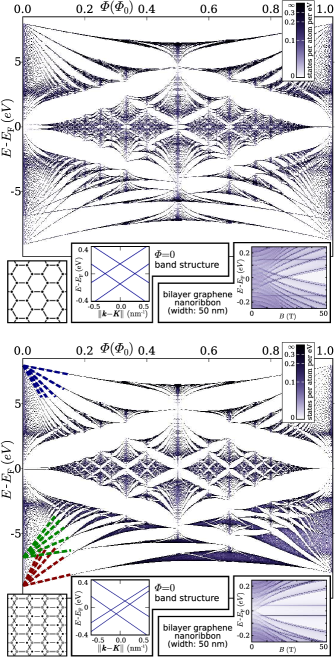
Figure 2: (Color online) Hofstadter butterfly of a bilayer graphene in two differently shifted configurations. Top panel: AA stacking (two layers exactly aligned). The band structure for this highly symmetric stacking (same rotational symmetry as for Bernal stacking in Fig. 1) shows the single-layer cone simply split up in energy. Bottom panel: Intermediate position between Bernal and AA stacking. The rotational symmetry is broken and the bands split into two cones at different offsets from the $K$ point and different energies. The straight lines overlaid at the energy minimum and maximum are the regular Landau levels of the massive bands. Near $E_{\mathrm{F}}$, one can make out the parabolic traces of the relativistic Landau levels and the horizontal lines of the SUSYLLs (see text). Insets at the lower right of each panel: DOS of a finite-width ribbon shows the corresponding behavior in each case.

The Hamiltonian without magnetic field—based on a tight-binding parametrization originally used for multiwalled carbon nanotubesLambin et al. (1994); Nemec and Cuniberti (2006)—consists of a contribution for nearest neighbors within a layer $\langle i,j\rangle$ and one for pairs of atoms located on different sheets $\left\langle\left\langle i,j\right\rangle\right\rangle$:

$$\mathcal{H} = -\sum_{\langle i,j\rangle}\gamma_{i,j}^{\operatorname{intra}}c^{{\dagger}}_{i}c^{\phantom{{\dagger}}}_{j}-\sum_{\left\langle\left\langle i,j\right\rangle\right\rangle}\gamma_{i,j}^{\operatorname{inter}}c^{{\dagger}}_{i}c^{\phantom{{\dagger}}}_{j}.$$

In absence of a magnetic field, the intralayer hopping is fixed to $\gamma_{i,j}^{\operatorname{intra}}=\gamma_{0}=2.66~{}\mathrm{\operatorname{eV}}$, while the interlayer hopping depends on the distance only,

$$\gamma_{i,j}^{\operatorname{inter}} = \beta\exp\left(\frac{a-\left|\boldsymbol{r}_{i}-\boldsymbol{r}_{j}\right|}{\delta}\right),$$

with $\beta=\gamma_{0}/8$, $a=3.34~{}\text{{\AA}}$, and $\delta=0.45~{}\text{{\AA}}$. A cutoff is chosen as $r_{\operatorname{cutoff}}=a+5\delta$. Following the Peierls substitution,Peierls (1933) the magnetic field $\boldsymbol{B}$ is now implemented by multiplying a magnetic phase factor to each link between two atoms $i$ and $j$:

$$\gamma_{i,j}\left(\boldsymbol{B}\right) = \gamma_{i,j}\left(\boldsymbol{B}=0\right)\exp\left(\mathrm{i}\frac{2\pi}{\Phi_{0}}\int_{\boldsymbol{r}_{i}}^{\boldsymbol{r}_{j}}\boldsymbol{A}_{B}\left(\boldsymbol{r}\right)\cdot\mathrm{d}\boldsymbol{r}\right),$$

where the integral is computed on a straight line between the atomic positions $\boldsymbol{r}_{i}$ and $\boldsymbol{r}_{j}$.

For the bilayer graphene, we arrive thus at a periodic Hamiltonian with a two-dimensional unit cell containing four atoms and spanning the area of one hexagonal graphene plaquette: $A_{\operatorname{plaquette}}=(3\sqrt{3}/2)d_{\operatorname{CC}}^{2}$, where $d_{\operatorname{CC}}=1.42~{}\text{{\AA}}$ is the intralayer distance between neighboring carbon atoms. The effect of a perpendicular magnetic field, measured in flux per plaquette $\Phi=A_{\operatorname{plaquette}}B$, can be calculated for commensurate values $\Phi=\left(p/q\right)\Phi_{0}$ ($p$, $q$ integers) by constructing a supercell of $q$ unit cells. The corresponding Bloch Hamiltonian $\mathcal{H}\left(\boldsymbol{k}\right)$ is a $4q\times 4q$ matrix that can be diagonalized for arbitrary values of $\boldsymbol{k}$ in the two-dimensional Brillouin zone of area $4\pi^{2}/qA_{\operatorname{plaquette}}$.

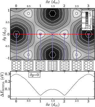
Figure 3: (Color online) Evolution of the split of the supersymmetric Landau level as a function of the displacement between the two graphene layers. Top panel: Magnitude of the split for displacements in two directions. The light spots correspond to Bernal stacking where the level is nearly degenerate. Bottom panel: Same data along a cut at $\delta y=0$. The small remaining split at the Bernal stacking configuration originates in the long-range interlayer hoppings contained in the parametrization. The small discontinuities are caused by the cutoff $r_{\operatorname{cut}}$. The calculation here was done at $\Phi=\Phi_{0}/256$, but proved to be independent of the magnetic field for values up to $\sim 0.05\Phi_{0}$.

To obtain the butterfly plots as displayed in Figs. 1 and 2, we chose $0\leqslant p\leqslant q=512$, reducing the fraction $p/q$ for efficiency. For each value of $\Phi$ the density of states was calculated from a histogram over the spectral values for a random sampling of $\boldsymbol{k}$ over the Brillouin zone. The number of sampling points was chosen individually for different values of $p$ to achieve convergence. In Figs. 1 and 2, the Hofstadter spectra of three differently aligned graphene bilayers are presented. The Bernal stacking (Fig. 1) stands out, as it is the configuration of layers in natural graphite.Bernal (1924); Hembacher et al. (2003) Alternative configurations like AA stacking were found in ab initio calculations to be energetically unfavorable;Aoki and Amawashi (2007) they can, however, be thought of as either mechanically shifted samples or sections of curved bilayers (e.g., sections of two shells in a large multiwall carbon nanotube) where the alignment unavoidably varies over distance. Compared to the Hofstadter butterfly of a single sheet of graphene,Rammal (1985) two asymmetries are visible in all three plots: The electron-hole symmetry ($E\leftrightarrow-E$) is broken down by the interlayer coupling already at zero magnetic field: while the lowest-energy states of a single graphene layer have constant phase over all atoms and can couple efficiently into symmetric and antisymmetric hybrid states of the bilayer system, the states at high energies have alternating phases for neighboring atoms, so interlayer hybridization is prohibited by the second-nearest-neighbor interlayer coupling. For low magnetic fields, two sets of Landau levels can therefore be observed at the bottom of the spectrum, indicating a split of the massive band of graphene at the $\Gamma$ point ($E_{\min}^{0}=-3\gamma_{0}$, $m^{\ast}_{0}=2\hbar^{2}/3\gamma_{0}d_{\operatorname{CC}}^{2}$) into two bands at different energies and with different effective masses [$E_{\min}^{\pm}\approx E_{\min}^{0}\pm 1.1~{}\mathrm{\operatorname{eV}}$, $m_{\pm}^{\ast}\approx m_{0}^{\ast}/(1\mp 2.1\beta/\gamma_{0})$, independent of the relative shift of the two layers; see the straight lines overlaid in the bottom panel of Fig. 2]. At the top of the spectrum, where the split is prohibited, only one degenerate set of Landau levels appears, as in single-layer graphene. The original periodic symmetry along the $B$-field axis at one flux quantum per graphene plaquette is broken down due to the smaller areas formed by interlayer loops. The breaking of this symmetry is comparably small in the AA stacking configuration (Fig. 2, top) where loops of the full plaquette area are dominant. In the two other configurations smaller loops are more dominant, so the periodicity is perturbed more severely. In the intermediate configuration (Fig. 2, bottom), the fractal patterns appear slightly smeared out for high magnetic fields, due to the reduced symmetry of the system.

The right insets of Figs. 1 and 2 display the spectra of (200,0) bilayer graphene nanoribbons,Nakada et al. (1996) each in a corresponding configuration, obtained by a method described beforeNemec and Cuniberti (2006) that allows handling of continuous magnetic fields. For low magnetic fields, these spectra are strongly influenced by finite-size effects.Wakabayashi et al. (1999) Only for magnetic fields larger than $B^{\ast}\approx 4\Phi_{0}/d^{2}$, which for a ribbon of width $d=50~{}\operatorname{nm}$ relates to $\sim 7~{}\mathrm{T}$, do the spectra of two-dimensional bilayer graphene begin to emerge. Prominent in all three insets are the dark, horizontal pairs of lines at the center, the supersymmetric Landau levels. While these represent discrete levels in two-dimensional graphene sheets, they are broadened by the finite width of the ribbon to a peak of the same shape as in carbon nanotubes.Lee and Novikov (2003); Nemec and Cuniberti (2006) The mesoscopic character of these split SUSYLLs in dependence on the width $W$ of the ribbon is captured by the functional form of the density of states:

$$\rho\left(E,B,W)\right. = f\left(\left(E-E_{0}\right)W,BW^{2}\right)$$

where $E_{0}$ is the position of the maximum.

Single-layer graphene is known to feature an anomalous supersymmetric Landau level at the Fermi energy.McClure (1956); Gusynin and Sharapov (2005); Ezawa (2006) Neglecting Zeeman splitting, this level is fourfold degenerate (twice spin, twice valley) and half filled. For bilayer graphene in Bernal stacking (Fig. 1) the SUSYLLs of the two layers have been shown to be protected by symmetry and to remain degenerate, giving in total an eightfold degeneracy.McCann and Fal’ko (2006) In Fig. 2, this degeneracy can be observed to be lifted for displaced bilayers, leading to a split of the SUSYLL into a bonding and an antibonding hybrid state in the two layers, each fourfold degenerate. The continuous evolution of the split for varying displacement of the two layers against each other is displayed in Fig. 3. The split reaches its maximum of $\Delta E\sim 0.3~{}\mathrm{\operatorname{eV}}$ for the AA-stacking configuration and is minimal for Bernal stacking. For simpler tight-binding parametrizations that take into account only first- and second-nearest-neighbor interlayer hoppings, the degeneracy in the Bernal configuration is known to be exact.McCann and Fal’ko (2006) Here, in contrast, this degeneracy is split by $\Delta E\sim 0.01~{}\mathrm{\operatorname{eV}}$ due to interlayer hoppings of a longer range, similar to the effect caused by second-nearest-neighbor interactions within one layer.McCann (2006)

In conclusion, we have developed a method that allows the nonperturbative implementation of a magnetic field in periodic systems with arbitrarily positioned atoms. A $\pi$ orbital parametrization for graphitic interlayer interactions with arbitrary displacements was then used to calculate the Hofstadter spectrum of bilayer graphene in various configurations, revealing common features like electron-hole symmetry breaking, and differences, especially in the breaking of the magnetic-field periodicity. A close look at the supersymmetric Landau level at low fields near the Fermi energy revealed a breaking of the previously found symmetry, resulting in a split of the level, depending on the lateral displacement of the two graphene layers against each other.

We acknowledge fruitful discussions with I. Adagideli, C. Berger, V. Fal’ko, F. Guinea and H. Schomerus. This work was funded by the Volkswagen Foundation under Grant No. I/78 340 and by the European Union program CARDEQ under Contract No. IST-021285-2. Support from the Vielberth Foundation is also gratefully acknowledged.

References

- Wallace (1947) P. R. Wallace, Phys. Rev. 71, 622 (1947).
- McClure (1956) J. W. McClure, Phys. Rev. 104, 666 (1956).
- Zheng and Ando (2002) Y. Zheng and T. Ando, Phys. Rev. B 65, 245420 (2002).
- Novoselov et al. (2005a) K. S. Novoselov, D. Jiang, F. Schedin, T. J. Booth, V. V. Khotkevich, S. V. Morozov, and A. K. Geim, Proc. Natl. Acad. Sci. 102, 10451 (2005a).
- Zhang et al. (2005) Y. Zhang, Y.-W. Tan, H. L. Stormer, and P. Kim, Nature 438, 201 (2005).
- Novoselov et al. (2005b) K. S. Novoselov, A. K. Geim, S. V. Morozov, D. Jiang, M. I. Katsnelson, I. V. Grigorieva, S. V. Dubonos, and A. A. Firsov, Nature 438, 197 (2005b).
- Zhang et al. (2006) Y. Zhang, Z. Jiang, J. P. Small, M. S. Purewal, Y.-W. Tan, M. Fazlollahi, J. D. Chudow, J. A. Jaszczak, H. L. Stormer, and P. Kim, Phys. Rev. Lett. 96, 136806 (2006).
- Gusynin and Sharapov (2005) V. P. Gusynin and S. G. Sharapov, Phys. Rev. Lett. 95, 146801 (2005).
- Kane and Mele (2005) C. L. Kane and E. J. Mele, Phys. Rev. Lett. 95, 226801 (2005).
- Peres et al. (2006) N. M. R. Peres, F. Guinea, and A. H. Castro Neto, Phys. Rev. B 73, 125411 (2006).
- Guinea et al. (2006) F. Guinea, A. H. Castro Neto, and N. M. R. Peres, Phys. Rev. B 73, 245426 (2006).
- Hasegawa and Kohmoto (2006) Y. Hasegawa and M. Kohmoto, Phys. Rev. B 74, 155415 (2006).
- McCann and Fal’ko (2006) E. McCann and V. I. Fal’ko, Phys. Rev. Lett. 96, 086805 (2006).
- Novoselov et al. (2006) K. S. Novoselov, E. McCann, S. V. Morozov, V. I. Fal’ko, M. I. Katsnelson, U. Zeitler, D. Jiang, F. Schedin, and A. K. Geim, Nat. Phys. 2, 177 (2006).
- Ohta et al. (2006) T. Ohta, A. Bostwick, T. Seyller, K. Horn, and E. Rotenberg, Science 313, 951 (2006).
- DiVincenzo and Mele (1984) D. P. DiVincenzo and E. J. Mele, Phys. Rev. B 29, 1685 (1984).
- Ezawa (2006) M. Ezawa, unpublished, eprint cond-mat/0606084.
- Peierls (1933) R. Peierls, Z. Phys. 80, 763 (1933).
- Hofstadter (1976) D. R. Hofstadter, Phys. Rev. B 14, 2239 (1976).
- Albrecht et al. (2001) C. Albrecht, J. H. Smet, K. von Klitzing, D. Weiss, V. Umansky, and H. Schweizer, Phys. Rev. Lett. 86, 147 (2001).
- Analytis et al. (2004) J. G. Analytis, S. J. Blundell, and A. Ardavan, Am. J. Phys. 72, 613 (2004).
- Rammal (1985) R. Rammal, J. Phys. (Paris) 46, 1345 (1985).
- Nemec and Cuniberti (2006) N. Nemec and G. Cuniberti, Phys. Rev. B 74, 165411 (2006).
- Bernal (1924) J. D. Bernal, Proc. R. Soc. London, Ser. A 106, 749 (1924).
- Trellakis (2003) A. Trellakis, Phys. Rev. Lett. 91, 056405 (2003).
- Cai and Galli (2004) W. Cai and G. Galli, Phys. Rev. Lett. 92, 186402 (2004).
- Lambin et al. (1994) P. Lambin, J. Charlier, and J. Michenaud, Electronic Structure of Coaxial Carbon Tubules (World Scientific, Singapore, 1994), pp. 130–134, ISBN 981-021887-7.
- Hembacher et al. (2003) S. Hembacher, F. J. Giessibl, J. Mannhart, and C. F. Quate, Proc. Natl. Acad. Sci. 100, 12539 (2003).
- Aoki and Amawashi (2007) M. Aoki and H. Amawashi, Solid State Comm. 142, 123 (2007).
- Nakada et al. (1996) K. Nakada, M. Fujita, G. Dresselhaus, and M. S. Dresselhaus, Phys. Rev. B 54, 17954 (1996).
- Wakabayashi et al. (1999) K. Wakabayashi, M. Fujita, H. Ajiki, and M. Sigrist, Phys. Rev. B 59, 8271 (1999).
- Lee and Novikov (2003) H.-W. Lee and D. S. Novikov, Phys. Rev. B 68, 155402 (2003).
- McCann (2006) E. McCann, Phys. Rev. B 74, 161403(R) (2006).