Gibbs states and the set of solutions of random constraint satisfaction problems

Abstract

An instance of a random constraint satisfaction problem defines a random subset ${\cal S}$ (the set of solutions) of a large product space ${\cal X}^{N}$ (the set of assignments). We consider two prototypical problem ensembles (random $k$-satisfiability and $q$-coloring of random regular graphs), and study the uniform measure with support on ${\cal S}$. As the number of constraints per variable increases, this measure first decomposes into an exponential number of pure states (‘clusters’), and subsequently condensates over the largest such states. Above the condensation point, the mass carried by the $n$ largest states follows a Poisson-Dirichlet process.

For typical large instances, the two transitions are sharp. We determine for the first time their precise location. Further, we provide a formal definition of each phase transition in terms of different notions of correlation between distinct variables in the problem.

The degree of correlation naturally affects the performances of many search/sampling algorithms. Empirical evidence suggests that local Monte Carlo Markov Chain strategies are effective up to the clustering phase transition, and belief propagation up to the condensation point. Finally, refined message passing techniques (such as survey propagation) may beat also this threshold.

Constraint satisfaction problems (CSPs) arise in a large spectrum of scientific disciplines. An instance of a CSP is said to be satisfiable if there exists an assignment of $N$ variables $(x_{1},x_{2},\dots,x_{N})\equiv\underline{x}$, $x_{i}\in{\cal X}$ (${\cal X}$ being a finite alphabet) which satisfies all the constraints within a given collection. The problem consists in finding such an assignment or show that the constraints are unsatisfiable. More precisely, one is given a set of functions $\psi_{a}:{\cal X}^{k}\to\{0,1\}$, with $a\in\{1,\dots,M\}\equiv[M]$ and of $k$-tuples of indices $\{i_{a}(1),\dots,i_{a}(k)\}\subseteq[N]$, and has to establish whether there exists $\underline{x}\in{\cal X}^{N}$ such that $\psi_{a}(x_{i_{a}(1)},\dots,x_{i_{a}(k)})=1$ for all $a$’s. In this article we shall consider two well known families of CSP’s (both known to be NP-complete [1]):

1. $k$-satisfiability ($k$-SAT) with $k\geq 3$. In this case ${\cal X}=\{0,1\}$. The constraints are defined by fixing a $k$-tuple $(z_{a}(1),\dots,z_{a}(k))$ for each $a$, and setting $\psi_{a}(x_{i_{a}(1)},\dots,x_{i_{a}(k)})=0$ if $(x_{i_{a}(1)},\dots,x_{i_{a}(k)})=(z_{a}(1),\dots,z_{a}(k))$ and $=1$ otherwise.

2. $q$-coloring ($q$-COL) with $q\geq 3$. Given a graph $G$ with $N$ vertices and $M$ edges, one is asked to assign colors $x_{i}\in{\cal X}\equiv\{1,\dots,q\}$ to the vertices in such a way that no edge has the same color at both ends.

The optimization (maximize the number of satisfied constraints) and counting (count the number of satisfying assignments) versions of this problems are defined straightforwardly. It is also convenient to represent CSP instances as factor graphs [2], i.e. bipartite graphs with vertex sets $[N]$, $[M]$ including an edge between node $i\in[N]$ and $a\in[M]$ if and only if the $i$-th variable is involved in the $a$-th constraint, cf. Fig. 1. This representation allows to define naturally a distance $d(i,j)$ between variable nodes.

Ensembles of random CSP’s (rCSP) were introduced (see e.g. [3]) with the hope of discovering generic mathematical phenomena that could be exploited in the design of efficient algorithms. Indeed several search heuristics, such as Walk-SAT [4] and ‘myopic’ algorithms [5] have been successfully analyzed and optimized over rCSP ensembles. The most spectacular advance in this direction has probably been the introduction of a new and powerful message passing algorithm (‘survey propagation’, SP) [6]. The original justification for SP was based on the (non-rigorous) cavity method from spin glass theory. Subsequent work proved that standard message passing algorithms (such as belief propagation, BP) can indeed be useful for some CSP’s [7, 8, 9]. Nevertheless, the fundamental reason for the (empirical) superiority of SP in this context remains to be understood and a major open problem in the field. Building on a refined picture of the solution set of rCSP, this paper provides a possible (and testable) explanation.

Figure 1: The factor graph of a small CSP allows to define the distance $d(i,j)$ between variables $x_{i}$ and $x_{j}$ (filled squares are constraints and empty circles variables). Here, for instance, $d(6,1)=2$ and $d(3,5)=1$.

We consider two ensembles that have attracted the majority of work in the field: $(i)$ random $k$-SAT: each $k$-SAT instance with $N$ variables and $M=N\alpha$ clauses is considered with the same probability; $(ii)$ $q$-COL on random graphs: the graph $G$ is uniformly random among the ones over $N$ vertices, with uniform degree $l$ (the number of constraints is therefore $M=Nl/2$).

0.1 Phase transitions in random CSP

It is well known that rCSP’s may undergo phase transitions as the number of constraints per variable $\alpha$ is varied. The best known of such phase transitions is the SAT-UNSAT one: as $\alpha$ crosses a critical value $\alpha_{\rm s}(k)$ (that can, in principle, depend on $N$), the instances pass from being satisfiable to unsatisfiable with high probability [10]. For $k$-SAT, it is known that $\alpha_{\rm s}(2)=1$. A conjecture based on the cavity method was put forward in [6] for all $k\geq 3$ that implied in particular the values presented in Table 1 and $\alpha_{\rm s}(k)=2^{k}\log 2-\frac{1}{2}(1+\log 2)+O(2^{-k})$ for large $k$ [11]. Subsequently it was proved that $\alpha_{\rm s}(k)\geq 2^{k}\log 2-O(k)$ confirming this asymptotic behavior [12]. An analogous conjecture for $q$-coloring was proposed in [13] yielding, for regular random graphs [14], the values reported in Table 1 and $l_{\rm s}(q)=2q\log{q}-\log{q}-1+o(1)$ for large $q$ (according to our convention, random graphs are whp uncolorable if $l\geq l_{\rm s}(q)$). It was proved in [15, 12] that $l_{\rm s}(q)=2q\log q-O(\log q)$.

Even more interesting and challenging are phase transitions in the structure of the set ${\cal S}\subseteq{\cal X}^{N}$ of solutions of rCSP’s (‘structural’ phase transitions). Assuming the existence of solutions, a convenient way of describing ${\cal S}$ is to introduce the uniform measure over solutions $\mu(\underline{x})$:

$$\mu(\underline{x})=\frac{1}{Z}\,\prod_{a=1}^{M}\psi_{a}(x_{i_{a}(1)},\dots,x_{i_{a}(k)})\,,$$ (1)

where $Z\geq 1$ is the number of solutions. Let us stress that, since ${\cal S}$ depends on the rCSP instance, $\mu(\,\cdot\,)$ is itself random.

Table 1: Critical connectivities for the dynamical, condensation and satisfiability transitions in k-SAT and q-COL

SAT	$\alpha_{\rm d}$	$\alpha_{\rm c}$	$\alpha_{\rm s}$[11]	COL	$l_{\rm d}$[16]	$l_{\rm c}$	$l_{\rm s}$[14]
$k=4$	$9.38$	$9.547$	$9.93$	$q=4$	$9$	$10$	$10$
$k=5$	$19.16$	$20.80$	$21.12$	$q=5$	$14$	$14$	$15$
$k=6$	$36.53$	$43.08$	$43.4$	$q=6$	$18$	$19$	$20$

We shall now introduce a few possible ‘global’ characterizations of the measure $\mu(\,\cdot\,)$. Each one of these properties has its counterpart in the theory of Gibbs measures and we shall partially adopt that terminology here [17].

In order to define the first of such characterizations, we let $i\in[N]$ be a uniformly random variable index, denote as $\underline{x}_{\ell}$ the vector of variables whose distance from $i$ is at least $\ell$, and by $\mu(x_{i}|\underline{x}_{\ell})$ the marginal distribution of $x_{i}$ given $\underline{x}_{\ell}$. Then we say that the measure (1) satisfies the uniqueness condition if, for any given $i\in[N]$,

$$\mathbb{E}\sup_{\underline{x}_{\ell},\underline{x}^{\prime}_{\ell}}\sum_{x_{i}\in{\cal X}}\left|\mu(x_{i}|\underline{x}_{\ell})-\mu(x_{i}|\underline{x}^{\prime}_{\ell})\right|\to 0\,.$$ (2)

as $\ell\to\infty$ (here and below the limit $N\to\infty$ is understood to be taken before $\ell\to\infty$). This expresses a ‘worst case’ correlation decay condition. Roughly speaking: the variable $x_{i}$ is (almost) independent of the far apart variables $\underline{x}_{\ell}$ irrespective is the instance realization and the variables distribution outside the horizon of radius $\ell$. The threshold for uniqueness (above which uniqueness ceases to hold) was estimated in [9] for random $k$-SAT, yielding $\alpha_{\rm u}(k)=(2\log k)/k[1+o(1)]$ (which is asymptotically close to the threshold for the pure literal heuristics) and in [18] for coloring implying $l_{\rm u}(q)=q$ for $q$ large enough (a ‘numerical’ proof of the same statement exists for small $q$). Below such thresholds BP can be proved to return good estimates of the local marginals of the distribution (1).

Notice that the uniqueness threshold is far below the SAT-UNSAT threshold. Furthermore, several empirical studies [19, 20] pointed out that BP (as well as many other heuristics [4, 5]) is effective up to much larger values of the clause density. In a remarkable series of papers [21, 6], statistical physicists argued that a second structural phase transition is more relevant than the uniqueness one. Following this literature, we shall refer to this as the ‘dynamic phase transition’ (DPT) and denote the corresponding threshold as $\alpha_{\rm d}(k)$ (or $l_{\rm d}(q)$). In order to precise this notion, we provide here two alternative formulations corresponding to two distinct intuitions. According to the first one, above $\alpha_{\rm d}(k)$ the variables $(x_{1},\dots,x_{N})$ become globally correlated under $\mu(\,\cdot\,)$. The criterion in (2) is replaced by one in which far apart variables $\underline{x}_{\ell}$ are themselves sampled from $\mu$ (‘extremality’ condition):

$$\mathbb{E}\sum_{\underline{x}_{\ell}}\mu(\underline{x}_{\ell})\sum_{x_{i}}\left|\mu(x_{i}|\underline{x}_{\ell})-\mu(x_{i})\right|\to 0\,.$$ (3)

as $\ell\to\infty$. The infimum value of $\alpha$ (respectively $l$) such that this condition is no longer fulfilled is the threshold $\alpha_{\rm d}(k)$ ($l_{\rm d}(k)$). Of course this criterion is weaker than the uniqueness one (hence $\alpha_{\rm d}(k)\geq\alpha_{\rm u}(k)$).

According to the second intuition, above $\alpha_{\rm d}(k)$, the measure (1) decomposes into a large number of disconnected ‘clusters’. This means that there exists a partition $\{A_{n}\}_{n=1\dots\cal N}$ of ${\cal X}^{N}$ (depending on the instance) such that: $(i)$ One cannot find $n$ such that $\mu(A_{n})\to 1$; $(ii)$ Denoting by $\partial_{\epsilon}A$ the set of configurations $\underline{x}\in{\cal X}^{N}\backslash A$ whose Hamming distance from $A$ is at most $N\epsilon$, we have $\mu(\partial_{\epsilon}A_{n})/\mu(A_{n})(1-\mu(A_{n}))\to 0$ exponentially fast in $N$ for all $n$ and $\epsilon$ small enough. Notice that the measure $\mu$ can be decomposed as

$$\mu(\,\cdot\,)=\sum_{n=1}^{{\cal N}}w_{n}\,\mu_{n}(\,\cdot\,)\,,$$ (4)

where $w_{n}\equiv\mu(A_{n})$ and $\mu_{n}(\,\cdot\,)\equiv\mu(\,\cdot\,|A_{n})$. We shall always refer to $\{A_{n}\}$ as the ‘finer’ partition with these properties.

The above ideas are obviously related to the performance of algorithms. For instance, the correlation decay condition in (3) is likely to be sufficient for approximate correctness of BP on random formulae. Also, the existence of partitions as above implies exponential slowing down in a large class of MCMC sampling algorithms.

Recently, some important rigorous results were obtained supporting this picture [22, 23]. However, even at the heuristic level, several crucial questions remain open. The most important concern the distribution of the weights $\{w_{n}\}$: are they tightly concentrated (on an appropriate scale) or not? A (somewhat surprisingly) related question is: can the absence of decorrelation above $\alpha_{\rm d}(k)$ be detected by probing a subset of variables bounded in $N$?

SP [6] can be thought as an inference algorithm for a modified graphical model that gives unit weight to each cluster [24, 20], thus tilting the original measure towards small clusters. The resulting performances will strongly depend on the distribution of the cluster sizes $w_{n}$. Further, under the tilted measure, $\alpha_{\rm d}(k)$ is underestimated because small clusters have a larger impact. The correct value was never determined (but see [16] for coloring). The authors of [25] undertook the technically challenging task of determining the cluster size distribution, without however clarifying several of its properties.

In this paper we address these issues, and unveil at least two unexpected phenomena. Our results are described in the next Section with a summary just below. Finally we will discuss the connection with the performances of SP. Some technical details of the calculation are collected in the last Section.

1 Results and discussion

The formulation in terms of extremality condition, cf. Eq. (3), allows for an heuristic calculation of the dynamic threshold $\alpha_{\rm d}(k)$. Previous attempts were based instead on the cavity method, that is an heuristic implementation of the definition in terms of pure state decomposition, cf. Eq. (4). Generalizing the results of [16], it is possible to show that the two calculations provide identical results. However, the first one is technically simpler and under much better control. As mentioned above we obtain, for all $k\geq 4$ a value of $\alpha_{\rm d}(k)$ larger than the one quoted in [6, 11].

Further we determined the distribution of cluster sizes $w_{n}$, thus unveiling a third ‘condensation’ phase transition at $\alpha_{\rm c}(k)\geq\alpha_{\rm d}(k)$ (strict inequality holds for $k\geq 4$ in SAT and $q\geq 4$ in coloring, see below). For $\alpha<\alpha_{\rm c}(k)$ the weights $w_{n}$ concentrate on a logarithmic scale (namely $-\log w_{n}$ is $\Theta(N)$ with $\Theta(N^{1/2})$ fluctuations). Roughly speaking the measure is evenly split among an exponential number of clusters.

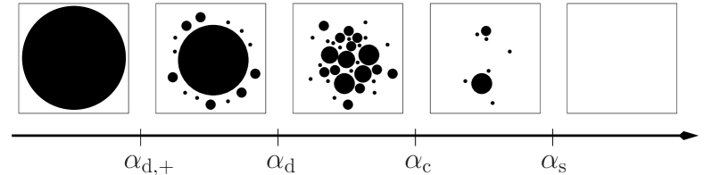
Figure 2: Pictorial representation of the different phase transitions in the set of solutions of a rCSP. At $\alpha_{{\rm d},+}$ some clusters appear, but for $\alpha_{{\rm d},+}<\alpha<\alpha_{\rm d}$ they comprise only an exponentially small fraction of solutions. For $\alpha_{\rm d}<\alpha<\alpha_{\rm c}$ the solutions are split among about $e^{N\Sigma_{*}}$ clusters of size $e^{Ns_{*}}$. If $\alpha_{\rm c}<\alpha<\alpha_{\rm s}$ the set of solutions is dominated by a few large clusters (with strongly fluctuating weights), and above $\alpha_{\rm s}$ the problem does not admit solutions any more.

For $\alpha>\alpha_{\rm c}(k)$ (and $<\alpha_{\rm s}(k)$) the measure is carried by a subexponential number of clusters. More precisely, the ordered sequence $\{w_{n}\}$ converges to a well known Poisson-Dirichlet process $\{w^{*}_{n}\}$, first recognized in the spin glass context by Ruelle [26]. This is defined by $w^{*}_{n}=x_{n}/\sum x_{n}$, where $x_{n}>0$ are the points of a Poisson process with rate $x^{-1-m(\alpha)}$ and $m(\alpha)\in(0,1)$. This picture is known in spin glass theory as ‘one step replica symmetry breaking’ (1RSB) and has been proven in Ref. [27] for some special models. The ‘Parisi 1RSB parameter’ $m(\alpha)$ is monotonically decreasing from $1$ to $0$ when $\alpha$ increases from $\alpha_{\rm c}(k)$, to $\alpha_{\rm s}(k)$, cf. Fig. 3.

Remarkably the condensation phase transition is also linked to an appropriate notion of correlation decay. If $i(1),\dots,i(n)\in[N]$ are uniformly random variable indices, then, for $\alpha<\alpha_{\rm c}(k)$ and any fixed $n$:

$$\mathbb{E}\sum_{\{x_{i(\cdot)}\}}\left|\mu(x_{i(1)}\dots x_{i(n)})-\mu(x_{i(1)})\cdots\mu(x_{i(n)})\right|\to 0$$ (5)

as $N\to\infty$. Conversely, the quantity on the left hand side remains positive for $\alpha>\alpha_{\rm c}(k)$. It is easy to understand that this condition is even weaker than the extremality one, cf. Eq. (3), in that we probe correlations of finite subsets of the variables. In the next two Sections we discuss the calculation of $\alpha_{\rm d}$ and $\alpha_{\rm c}$.

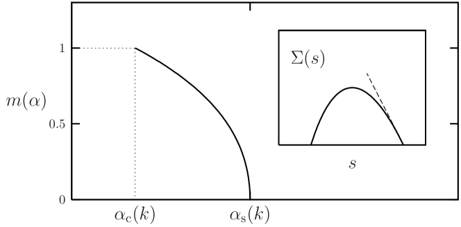
Figure 3: The Parisi 1RSB parameter $m(\alpha)$ as a function of the constraint density $\alpha$. In the inset, the complexity $\Sigma(s)$ as a function of the cluster entropy for $\alpha=\alpha_{\rm s}(k)-0.1$ (the slope at $\Sigma(s)=0$ is $-m(\alpha)$). Both curves have been computed from the large $k$ expansion.

1.1 Dynamic phase transition and Gibbs measure extremality

A rigorous calculation of $\alpha_{\rm d}(k)$ along any of the two definitions provided above, cf. Eqs. (3) and (4) remains an open problem. Each of the two approaches has however an heuristic implementation that we shall now describe. It can be proved that the two calculations yield equal results as further discussed in the last Section of the paper.

The approach based on the extremality condition in (3) relies on an easy-to-state assumption, and typically provides a more precise estimate. We begin by observing that, due to the Markov structure of $\mu(\,\cdot\,)$, it is sufficient for Eq. (3) to hold that the same condition is verified by the correlation between $x_{i}$ and the set of variables at distance exactly $\ell$ from $i$, that we shall keep denoting as $\underline{x}_{\ell}$. The idea is then to consider a large yet finite neighborhood of $i$. Given $\bar{\ell}\geq\ell$, the factor graph neighborhood of radius $\bar{\ell}$ around $i$ converges in distribution to the radius–$\bar{\ell}$ neighborhood of the root in a well defined random tree factor graph $T$.

For coloring of random regular graphs, the correct limiting tree model $T$ is coloring on the infinite $l$-regular tree. For random $k$-SAT, $T$ is defined by the following construction. Start from the root variable node and connect it to $l$ new function nodes (clauses), $l$ being a Poisson random variable of mean $k\alpha$. Connect each of these function nodes with $k-1$ new variables and repeat. The resulting tree is infinite with non-vanishing probability if $\alpha>1/k(k-1)$. Associate a formula to this graph in the usual way, with each variable occurrence being negated independently with probability $1/2$.

The basic assumption within the first approach is that the extremality condition in (3) can be checked on the correlation between the root and generation-$\ell$ variables in the tree model. On the tree, $\mu(\,\cdot\,)$ is defined to be a translation invariant Gibbs measure [17] associated to the infinite factor graph $T$ (which provides a specification). The correlation between the root and generation-$\ell$ variables can be computed through a recursive procedure (defining a sequence of distributions $\overline{P}_{\ell}$, see Eq. (15) below). The recursion can be efficiently implemented numerically yielding the values presented in Table 1 for $k$ (resp. $q$)$=4,5,6$. For large $k$ (resp. $q$) one can formally expand the equations on $P_{\ell}$ and obtain

$$\alpha_{\rm d}(k) = \frac{2^{k}}{k}\left[\log k+\log\log k+\gamma_{\rm d}+O\left(\frac{\log\log k}{\log k}\right)\right]\,$$ (6)

$$l_{\rm d}(q) = q\ \left[\log q+\log\log q+\gamma_{\rm d}+o(1)\right]$$ (7)

with $\gamma_{\rm d}=1$ (under a technical assumption on the structure of $P_{\ell}$).

The second approach to the determination of $\alpha_{\rm d}(k)$ is based on the ‘cavity method’ [6, 25]. It begins by assuming a decomposition in pure states of the form (4) with two crucial properties: $(i)$ If we denote by $W_{n}$ the size of the $n$-th cluster (and hence $w_{n}=W_{n}/\sum W_{n}$), then the number of clusters of size $W_{n}=e^{Ns}$ grows approximately as $e^{N\Sigma(s)}$; $(ii)$ For each single-cluster measure $\mu_{n}(\,\cdot\,)$, a correlation decay condition of the form (3) holds.

The approach aims at determining the rate function $\Sigma(s)$, ‘complexity’: the result is expressed in terms of the solution of a distributional fixed point equation. For the sake of simplicity we describe here the simplest possible scenario resulting from such a calculation, cf. Fig. 4. For $\alpha<\alpha_{{\rm d},-\infty}(k)$ the cavity fixed point equation does not admit any solution: no clusters are present. At $\alpha_{{\rm d},-\infty}(k)$ a solution appears, eventually yielding, for $\alpha>\alpha_{{\rm d},+}$ a non-negative complexity $\Sigma(s)$ for some values of $s\in{\mathbb{R}}_{+}$. The maximum and minimum such values will be denoted by $s_{\rm max}$ and $s_{\rm min}$. At a strictly larger value $\alpha_{{\rm d},0}(k)$, $\Sigma(s)$ develops a stationary point (local maximum). It turns out that $\alpha_{{\rm d},0}(k)$ coincides with the threshold computed in [6, 11, 14]. In particular $\alpha_{{\rm d},0}(4)\approx 8.297$, $\alpha_{{\rm d},0}(5)\approx 16.12$, $\alpha_{{\rm d},0}(6)\approx 30.50$ and $l_{{\rm d},0}(4)=9$, $l_{{\rm d},0}(5)=13$, $l_{{\rm d},0}(6)=17$. For large $k$ (resp. $q$), $\alpha_{{\rm d},0}(k)$ admits the same expansion as in Eqs. (6), (7) with $\gamma_{{\rm d},0}=1-\log 2$. However, up to the larger value $\alpha_{\rm d}(k)$, the appearance of clusters is irrelevant from the point of view of $\mu(\,\cdot\,)$. In fact, within the cavity method it can be shown that $e^{N[s+\Sigma(s)]}$ remains exponentially smaller than the total number of solutions $Z$: most of the solutions are in a single “cluster”. The value $\alpha_{\rm d}(k)$ is determined by the appearance of a point $s_{*}$ with $\Sigma^{\prime}(s_{*})=-1$ on the complexity curve. Correspondingly, one has $Z\approx e^{N[\Sigma(s_{*})+s_{*}]}$: most of the solutions are comprised in clusters of size about $e^{Ns_{*}}$. The entropy per variable $\phi=\lim_{\begin{subarray}{c}N\end{subarray}\rightarrow\infty}N^{-1}\log Z$ remains analytic at $\alpha_{\rm d}(k)$.

1.2 Condensation phase transition

As $\alpha$ increases above $\alpha_{\rm d}$, $\Sigma(s_{*})$ decreases: clusters of highly correlated solutions may no longer satisfy the newly added constraints. In the inset of Fig. 5 we show the $\alpha$ dependency of $\Sigma(s_{*})$ for $4$-SAT. In the large $k$ limit, with $\alpha=\rho\,2^{k}$ we get $\Sigma(s^{*})=\log 2-\rho-\log 2\,e^{-k\rho}+O(2^{-k})$, and $s_{*}=\log 2\,e^{-k\rho}+O(2^{-k})$.

The condensation point $\alpha_{\rm c}(k)$ is the value of $\alpha$ such that $\Sigma(s_{*})$ vanishes: above $\alpha_{\rm c}(k)$, most of the measure is contained in a sub-exponential number of large clusters. Our estimates for $\alpha_{\rm c}(k)$ are presented in Table 1 (see also Fig. 4 for $\Sigma(s)$ in the $6$-coloring) while in the large-$k$ limit we obtain $\alpha_{\rm c}(k)=2^{k}\log 2-\frac{3}{2}\log 2+O(2^{-k})$ [recall that the SAT-UNSAT transition is at $\alpha_{\rm s}(k)=2^{k}\log 2-\frac{1+\log 2}{2}+O(2^{-k})$] and $l_{\rm c}(q)=2q\log q-\log q-2\log 2+o(1)$ [with the COL-UNCOL transition at $l_{\rm s}(q)=2q\log q-\log q-1+o(1)$].

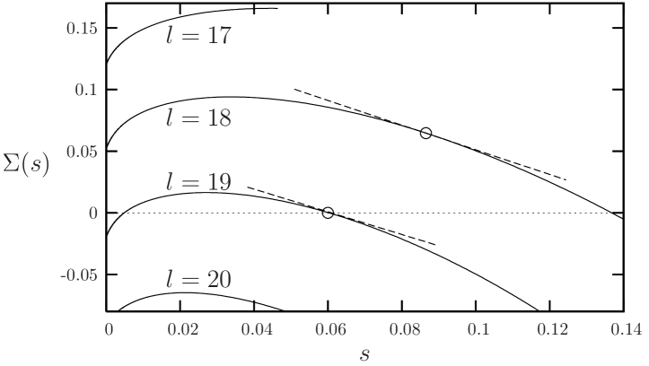
Figure 4: The complexity function (the number of clusters with entropy density $s$ is $e^{N\Sigma(s)}$) for the $6$-colorings of $l$-regular graphs with $l\in\{17,18,19,20\}$. Circles indicate the dominating states with entropy $s_{*}$; the dashed lines have slopes $\Sigma^{\prime}(s_{*})=-1$ for $l=18$ and $\Sigma^{\prime}(s_{*})=-0.92$ for $l=19$. The dynamic phase transition is $l_{\rm d}(6)=18$, the condensation one $l_{\rm d}(6)=19$, and the SAT-UNSAT one $l_{\rm s}(6)=20$.

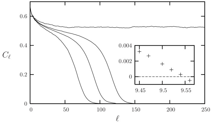
Figure 5: Correlation function (3) between the root and generation $\ell$ variables in a random $k$-SAT tree formula. Here $k=4$ and (from bottom to top) $\alpha=9.30$, $9.33$, $9.35$, $9.40$ (recall that $\alpha_{\rm d}(4)\approx 9.38$). In the inset, the complexity $\Sigma(s_{*})$ of dominant clusters as a function of $\alpha$ for $4$-SAT.

Technically the size of dominating clusters is found by maximizing $\Sigma(s)+s$ over the $s$ interval on which $\Sigma(s)\geq 0$. For $\alpha\in[\alpha_{\rm c}(k),\alpha_{\rm s}(k)]$, the maximum is reached at $s_{\rm max}$, with $\Sigma(s_{\rm max})=0$ yielding $\phi=s_{\rm max}$. It turns out that the solutions are comprised within a finite number of clusters, with entropy $e^{Ns_{\rm max}+\Delta}$, where $\Delta=\Theta(1)$. The shifts $\Delta$ are asymptotically distributed according to a Poisson point process of rate $e^{-m(\alpha)\Delta}$ with $m(\alpha)=-\Sigma^{\prime}(s_{\rm max})$. This leads to the Poisson Dirichlet distribution of weights discussed above. Finally, the entropy per variable $\phi$ is non-analytic at $\alpha_{\rm c}(k)$.

Let us conclude by stressing two points. First, we avoided the $3$-SAT and $3$-coloring cases. These cases (as well as the $3$-coloring on Erdös-Rényi graphs [25]) are particular in that the dynamic transition point $\alpha_{\rm d}$ is determined by a local instability (a Kesten-Stigum [29] condition, see also [21]), yielding $\alpha_{\rm d}(3)\approx 3.86$ and $l_{\rm d}(3)=6$ (the case $l=5$, $q=3$ being marginal). Related to this is the fact that $\alpha_{\rm c}=\alpha_{\rm d}$: throughout the clustered phase, the measure is dominated by a few large clusters (technically, $\Sigma(s_{*})<0$ for all $\alpha>\alpha_{\rm d}$). Second, we did not check the ‘local stability’ of the 1RSB calculation. By analogy with [30], we expect that an instability can modify the curve $\Sigma(s)$ but not the values of $\alpha_{\rm d}$ and $\alpha_{\rm c}$.

1.3 Algorithmic implications

Two message passing algorithms were studied extensively on random $k$-SAT: belief propagation (BP) and survey propagation (SP) (mixed strategies were also considered in [19, 20]). A BP message $\nu_{u\to v}(x)$ between nodes $u$ and $v$ on the factor graph is usually interpreted as the marginal distribution of $x_{u}$ (or $x_{v}$) in a modified graphical model. An SP message is instead a distribution over such marginals $P_{u\to v}(\nu)$. The empirical superiority of SP is usually attributed to the existence of clusters [6]: the distribution $P_{u\to v}(\nu)$ is a ‘survey’ of the marginal distribution of $x_{u}$ over the clusters. As a consequence, according to the standard wisdom, SP should outperform BP for $\alpha>\alpha_{\rm d}(k)$.

This picture has however several problems. Let us list two of them. First, it seems that essentially local algorithms (such as message passing ones) should be sensitive only to correlations among finite subsets of the variables, and these remain bounded up to the condensation transition. Recall in fact that the extremality condition in (3) involves a number of variables unbounded in $N$, while the weaker in (5) is satisfied up to $\alpha_{\rm c}(k)$.

Secondly, it would be meaningful to weight uniformly the solutions when computing the surveys $P_{u\to v}(\nu)$. In the cavity method jargon, this corresponds to using a 1RSB Parisi parameter $r=1$ instead of $r=0$ as is done in [6]. It is a simple algebraic fact of the cavity formalism that for $r=1$ the means of the SP surveys satisfy the BP equations. Since the means are the most important statistics used by SP to find a solution, BP should perform roughly as SP.

Figure 6: Performance of BP heuristics on random $4$-SAT formulae. The residual entropy per spin $N^{-1}\log Z$ (here we estimate it within Bethe approximation) as a function of the fraction of fixed variables. $t_{\text{max}}=20$ in these experiments.

Both arguments suggest that BP should perform well up to the condensation point $\alpha_{\rm c}(k)$. We tested this conclusion on $4$-SAT at $\alpha=9.5\in(\alpha_{\rm d}(4),\alpha_{\rm c}(4))$, through the following numerical experiment, cf. Fig. 6. $(i)$ Run BP for $t_{\rm max}$ iterations. $(ii)$ Compute the BP estimates $\nu_{i}(x)$ for the single bit marginals and choose the one with largest bias. $(iii)$ Fix $x_{i}=0$ or $1$ with probabilities $\nu_{i}(0)$, $\nu_{i}(1)$. $(iv)$ Reduce the formula accordingly (i.e. eliminate the constraints satisfied by the assignment of $x_{i}$ and reduce the ones violated). This cycle is repeated until a solution is found or a contradiction is encountered. If the marginals $\nu_{i}(\,\cdot\,)$ were correct, this procedure would provide a satisfying assignment sampled uniformly from $\mu(\,\cdot\,)$. In fact we found a solution with finite probability (roughly $0.4$), despite the fact that $\alpha>\alpha_{\rm d}(4)$. The experiment was repeated at $\alpha=9$ with a similar fraction of successes (more data on the success probability will be reported in [31]).

Above the condensation transition, correlations become too strong and the BP fixed point no longer describes the measure $\mu$. Indeed the same algorithm proved unsuccessful at $\alpha=9.7\in(\alpha_{\rm c}(4),\alpha_{\rm s}(4))$. As mentioned above, SP can be regarded as an inference algorithm in a modified graphical model that weights preferentially small clusters. More precisely, it selects clusters of size $e^{N\bar{s}}$ with $\bar{s}$ maximizing the complexity $\Sigma(s)$. With respect to the new measure, the weak correlation condition in (5) still holds and allows to perform inference by message passing.

Within the cavity formalism, the optimal choice would be to take $r\approx m(\alpha)\in[0,1)$. Any parameter corresponding to a non-negative complexity $r\in[0,m(\alpha)]$ should however give good results. SP corresponds to the choice $r=0$ that has some definite computational advantages, since messages have a compact representation in this case (they are real numbers).

2 Cavity formalism, tree reconstruction and SP

This Section provides some technical elements of our computation. The reader not familiar with this topic is invited to further consult Refs. [6, 11, 25, 32] for a more extensive introduction. The expert reader will find a new derivation, and some hints of how we overcame technical difficulties. A detailed account shall be given in [31, 33].

On a tree factor graph, the marginals of $\mu(\,\cdot\,)$, Eq. (1) can be computed recursively. The edge of the factor graph from variable node $i$ to constraint node $a$ (respectively from $a$ to $i$) carries “message” $\overline{\eta}_{i\to a}$ ($\overline{\nu}_{a\to i}$), a probability measure on ${\cal X}$ defined as the marginal of $x_{i}$ in the modified graphical model obtained by deleting constraint node $a$ (resp. all constraint nodes around $i$ apart from $a$). The messages are determined by the equations

$$\!\!\overline{\eta}_{i\to a}(x_{i})\!\!\! = \!\!\!\frac{1}{z_{i\to a}(\{\overline{\nu}_{b\to i}\})}\prod_{b\in\partial i\setminus a}\overline{\nu}_{b\to i}(x_{i})\,,$$ (8)

$$\!\!\overline{\nu}_{a\to i}(x_{i})\!\!\! = \!\!\!\frac{1}{\widehat{z}_{a\to i}(\{\overline{\eta}_{j\to a}\})}\sum_{\underline{x}_{\partial a\setminus i}}\!\!\psi_{a}(\underline{x}_{\partial a})\!\!\!\prod_{j\in\partial a\setminus i}\!\!\overline{\eta}_{j\to a}(x_{j})\,,$$ (9)

where $\partial u$ is the set of nodes adjacent to $u$, $\setminus$ denotes the set subtraction operation, and $\underline{x}_{A}=\{x_{j}:j\in A\}$. These are just the BP equations for the model (1). The constants $z_{i\to a}$, $\widehat{z}_{a\to i}$ are uniquely determined from the normalization conditions $\sum_{x_{i}}\overline{\eta}_{i\to a}(x_{i})=\sum_{x_{i}}\overline{\nu}_{a\to i}(x_{i})=1$. In the following we refer to these equations by introducing functions $f_{i\to a}(\,\cdot\,)$, $f_{a\to i}(\,\cdot\,)$ such that

$$\overline{\eta}_{i\to a}=f_{i\to a}(\{\overline{\nu}_{b\to i}\}_{b\in\partial i\setminus a})\ ,\ \ \overline{\nu}_{a\to i}=f_{a\to i}(\{\overline{\eta}_{j\to a}\}_{j\in\partial a\setminus i})\ ,$$ (10)

The marginals of $\mu$ are then computed from the solution of these equations. For instance $\mu(x_{i})$ is a function of the messages $\overline{\nu}_{a\to i}$ from neighboring function nodes.

The log-number of solutions, $\log Z$, can be expressed as a sum of contributions which are local functions of the messages that solve Eqs. (8), (9)

$$\log Z= \sum_{a}\log z_{a}(\{\overline{\eta}_{i\to a}\})+\sum_{i}\log z_{i}(\{\overline{\nu}_{a\to i}\})+$$

$$-\sum_{(ai)}\log z_{ai}(\overline{\eta}_{i\to a},\overline{\nu}_{a\to i})$$ (11)

where the last sum is over undirected edges in the factor graph and

$$z_{a} \equiv\sum_{\underline{x}_{\partial a}}\psi_{a}(\underline{x}_{\partial a})\prod_{i\in\partial a}\overline{\eta}_{i\to a}(x_{i})\,,$$

$$z_{i} \equiv\sum_{x_{i}}\prod_{a\in\partial i}\overline{\nu}_{a\to i}(x_{i})\,,\qquad z_{ai}\equiv\sum_{x_{i}}\overline{\eta}_{i\to a}(x_{i})\overline{\nu}_{a\to i}(x_{i})\,.$$

Each term $z$ gives the change in the number of solutions when merging different subtrees (for instance $\log z_{i}$ is the change in entropy when the subtrees around $i$ are glued together). This expression coincides with the Bethe free-energy [34] as expressed in terms of messages.

In order to move from trees to loopy graphs, we first consider an intermediate step in which the factor graph is still a tree but a subset of the variables, $\underline{x}_{\mbox{\tiny B}}=\{x_{j}:j\in{\rm B}\}$ is fixed. We are therefore replacing the measure $\mu(\,\cdot\,)$, cf. Eq. (1), with the conditional one $\mu(\,\cdot\,|\underline{x}_{\mbox{\tiny B}})$. In physics terms, the variables in $\underline{x}_{\mbox{\tiny B}}$ specify a boundary condition.

Notice that the measure $\mu(\,\cdot\,|\underline{x}_{\mbox{\tiny B}})$ still factorizes according to (a subgraph of) the original factor graph. As a consequence, the conditional marginals $\mu(x_{i}|\underline{x}_{\mbox{\tiny B}})$ can be computed along the same lines as above. The messages $\eta_{i\to a}^{\underline{x}_{\mbox{\tiny B}}}$ and $\nu_{a\to i}^{\underline{x}_{\mbox{\tiny B}}}$ obey Eqs. (10), with an appropriate boundary condition for messages from ${\rm B}$. Also, the number of solutions that take values $\underline{x}_{\mbox{\tiny B}}$ on $j\in B$ (call it $Z(\underline{x}_{\mbox{\tiny B}})$) can be computed using Eq. (11).

Next, we want to consider the boundary variables themselves as random variables. More precisely, given $r\in{\mathbb{R}}$, we let the boundary to be $\underline{x}_{\mbox{\tiny B}}$ with probability

$$\widetilde{\mu}(\underline{x}_{\mbox{\tiny B}})=\frac{Z(\underline{x}_{\mbox{\tiny B}})^{r}}{{\cal Z}(r)}\ ,$$ (12)

where ${\cal Z}(r)$ enforces the normalization $\sum_{\underline{x}_{\mbox{\tiny B}}}\widetilde{\mu}(\underline{x}_{\mbox{\tiny B}})=1$. Define $P_{i\to a}(\eta)$ as the probability density of $\eta_{i\to a}^{\underline{x}_{\mbox{\tiny B}}}$ when $\underline{x}_{\mbox{\tiny B}}$ is drawn from $\widetilde{\mu}$, and similarly $Q_{a\to i}(\nu)$. One can show that Eq. (8) implies the following relation between messages distributions

$$P_{i\to a}(\eta)=\frac{1}{{\cal Z}_{i\to a}}\int\!\!\!\prod_{b\in\partial i\setminus a}\!\!{\rm d}Q_{b\to i}(\nu_{b})\,\delta[\eta-f_{i\to a}(\{\nu_{b}\})]\,z_{i\to a}(\{\nu_{b}\})^{r},$$ (13)

where $f_{i\to a}$ is the function defined in Eq. (10), $z_{i\to a}$ is determined by Eq. (8), and ${\cal Z}_{i\to a}$ is a normalization. A similar equation holds for $Q_{a\to i}(\nu)$. These coincide with the “1RSB equations” with Parisi parameter $r$. Survey propagation (SP) corresponds to a particular parameterization of Eq. (13) (and the analogous one expressing $Q_{a\to i}$ in terms of the $P$’s) valid for $r=0$.

The log-partition function $\Phi(r)=\log{\cal Z}(r)$ admits an expression that is analogous to Eq. (11),

$$\log{\cal Z}(r)= \sum_{a}\log{\cal Z}_{a}(\{P_{i\to a}\})+\sum_{i}\log{\cal Z}_{i}(\{Q_{a\to i}\})+$$

$$-\sum_{ai}\log{\cal Z}_{ai}(P_{i\to a},Q_{a\to i})$$ (14)

where the ‘shifts’ ${\cal Z}(\cdots)$ are defined through moments of order $r$ of the $z$’s, and sums run over vertices not in ${\rm B}$. For instance ${\cal Z}_{ai}$ is the expectation of $z_{ai}(\eta,\nu)^{r}$ when $\eta$, $\nu$ are independent random variables with distribution (respectively) $P_{i\to a}$ and $Q_{a\to i}$. The (Shannon) entropy of the distribution $\widetilde{\mu}$ is given by $\Sigma(r)=\Phi(r)-r\Phi^{\prime}(r)$.

As mentioned, the above derivation holds for tree factor graphs. Nevertheless, the local recursion equations (10), (13) can be used as an heuristics on loopy factor graphs as well. Further, although we justified Eq. (13) through the introduction of a random boundary condition $\underline{x}_{\mbox{\tiny B}}$, we can take ${\rm B}=\emptyset$ and still look for non-degenerate solutions of such equations.

Starting from an arbitrary initialization of the messages, the recursions are iterated until an approximate fixed point is reached. After convergence, the distributions $P_{i\to a}$, $Q_{a\to i}$ can be used to evaluate the potential $\Phi(r)$, cf. Eq. (14). From this we compute the complexity function $\Sigma(r)\equiv\Phi(r)-r\Phi^{\prime}(r)$, that gives access to the decomposition of $\mu(\,\cdot\,)$ in pure states. More precisely, $\Sigma(r)$ is the exponential growth rate of the number of states with internal entropy $s=\Phi^{\prime}(r)$. This is how curves such as in Fig. 4 are traced.

In practice it can be convenient to consider the distributions of messages $P_{i\to a}$, $Q_{a\to i}$ with respect to the graph realization. This approach is sometimes referred to as ‘density evolution’ in coding theory. If one consider a uniformly random directed edge $i\to a$ (or $a\to i$) in a rCSP instance, the corresponding message will be a random variable. After $t$ parallel updates according to Eq. (13), the message distribution converges (in the $N\to\infty$ limit) to a well defined law ${\cal P}_{t}$ (for variable to constraint messages) or ${\cal Q}_{t}$ (for constraint to variable). As $t\to\infty$, these converge to a fixed point ${\cal P}$, ${\cal Q}$ that satisfy the distributional equivalent of Eq. (13).

To be definite, let us consider the case of graph coloring. Since the compatibility functions are pairwise in this case (i.e. $k=2$ in Eq. (1)), the constraint-to-variable messages can be eliminated and Eq. (13) takes the form

$$P_{i\to j}(\eta)\propto\int\!\!\!\prod_{l\in\partial i\setminus j}\!\!{\rm d}P_{l\to i}(\eta_{l})\,\delta\left[\eta-f(\{\eta_{l}\})\right]z(\{\eta_{l}\})^{r}\,,$$

where $f$ is defined by $\eta(x)=z^{-1}\prod_{l}1-\eta_{l}(x)$ and $z$ by normalization. The distribution of $P_{i\to j}$ is then assumed to satisfy a distributional version of the last equation. In the special case of random regular graphs, a solution is obtained by assuming that $P_{i\to j}$ is indeed independent of the graph realization and of $i,j$. One has therefore simply to set $P_{i\to j}=P$ in the above and solve it for $P$.

In general, finding messages distributions ${\cal P}$, ${\cal Q}$ that satisfy the distributional version of Eq. (13) is an extremely challenging task, even numerically. We adopted the population dynamics method [32] which consists in representing the distributions by samples (this is closely related to particle filters in statistics). For instance, one represents ${\cal P}$ by a sample of $P$’s, each encoded as a list of $\eta$’s. Since computer memory drastically limits the samples size, and thus the precision of the results, we worked in two directions: $(1)$ We analytically solved the distributional equations for large $k$ (in the case of $k$-SAT) or $q$ ($q$-coloring); $(2)$ We identified and exploited simplifications arising for special values of $r$.

Let us briefly discuss point $(2)$. Simplifications emerge for $r=0$ and $r=1$. The first case correspond to SP: Refs. [6, 11] showed how to compute efficiently $\Sigma(r=0)$ through population dynamics. Building on this, we could show that the clusters internal entropy $s(r=0)$ can be computed at a small supplementary cost (see [31]).

The value $r=1$ corresponds instead to the ‘tree reconstruction’ problem [35]: In this case $\widetilde{\mu}(\underline{x}_{\mbox{\tiny B}})$, cf. Eq. (12), coincides with the marginal of $\mu$. Averaging Eq. (13) (and the analogous one for $Q_{a\to i}$) one obtains the BP equations (8), (9), e.g. $\int{\rm d}P_{i\to a}(\eta)\ \eta=\overline{\eta}_{i\to a}$. These remark can be used to show that the constrained averages

$$\overline{P}(\eta,\overline{\eta})=\int{\rm d}{\cal P}[P]\ P(\eta)\ \delta\left(\overline{\eta}-\int{\rm d}P(\eta^{\prime})\eta^{\prime}\right)\ ,$$ (15)

and $\overline{Q}(\nu,\overline{\nu})$ (defined analogously) satisfy closed equations which are much easier to solve numerically.

- [1] Garey MR and Johnson DS (1979) Computers and Intractability: A Guide to the Theory of NP-Completenes (Freeman, New York).
- [2] Kschischang FR, Frey BJ and Loeliger H-A (2001) IEEE Trans. Inform. Theory 47, 498-519.
- [3] Franco J and Paull M (1983) Discrete Appl. Math 5, 77-87.
- [4] Selman B, Kautz HA and Cohen B (1994) Proc. of AAAI-94, Seattle.
- [5] Achlioptas D and Sorkin GB (2000) Proc. of the Annual Symposium on the Foundations of Computer Science, Redondo Beach, CA.
- [6] Mézard M, Parisi G and Zecchina R (2002) Science 297, 812-815.
- [7] Bayati M, Shah D and Sharma M (2006) Proc. of International Symposium on Information Theory, Seattle.
- [8] Gamarnik D and Bandyopadhyay A (2006) Proc. of the Symposium on Discrete Algorithms, Miami.
- [9] Montanari A and Shah D (2007) Proc. of the Symposium on Discrete Algorithms, New Orleans.
- [10] Friedgut E (1999) J. Amer. Math. Soc. 12, 1017-1054.
- [11] Mertens S, Mézard M and Zecchina R (2006) Rand. Struct. and Alg. 28, 340-373.
- [12] Achlioptas D, Naor A and Peres Y (2005) Nature 435, 759-764.
- [13] Mulet R, Pagnani A, Weigt M and Zecchina R (2002) Phys. Rev. Lett. 89, 268701.
- [14] Krzakala F, Pagnani A and Weigt M (2004) Phys. Rev. E 70, 046705.
- [15] Luczak T (1991) Combinatorica 11, 45-54.
- [16] Mézard M and Montanari A (2006) J. Stat. Phys. 124, 1317-1350.
- [17] Georgii HO (1988) Gibbs Measures and Phase Transitions (De Gruyter, Berlin).
- [18] Jonasson J (2002) Stat. and Prob. Lett. 57, 243-248.
- [19] Aurell E, Gordon U and Kirkpatrick S (2004) Proc. of Neural Information Processing Symposium, Vancouver.
- [20] Maneva EN, Mossel E and Wainwright MJ (2005) Proc. of the Symposium on Discrete Algorithms, Vancouver.
- [21] Biroli G, Monasson R and Weigt M (2000) Eur. Phys. J. B 14, 551-568.
- [22] Mézard M, Mora T and Zecchina R (2005) Phys. Rev. Lett. 94, 197205.
- [23] Achlioptas D and Ricci-Tersenghi F (2006) Proc. of the Symposyum on the Theory of Computing, Washington.
- [24] Braunstein A and Zecchina R (2004) J. Stat. Mech., P06007.
- [25] Mézard M, Palassini M and Rivoire O (2005) Phys. Rev. Lett. 95, 200202.
- [26] Ruelle D (1987) Commun. Math. Phys. 108, 225-239.
- [27] Talagrand M (2000) C. R. Acad. Sci. Paris, Ser. I 331, 939-942.
- [28] Montanari A and Semerjian G, In preparation.
- [29] Kesten H and Stigum BP (1966) Ann. Math. Statist. 37, 1463-1481. Kesten H and Stigum BP (1966) J. Math. Anal. Appl. 17, 309-338.
- [30] Montanari A and Ricci-Tersenghi F (2004) Phys. Rev. B 70, 134406.
- [31] Montanari A, Ricci-Tersenghi F and Semerjian G, In preparation.
- [32] Mézard M and Parisi G (2001) Eur. Phys. J. B 20, 217-233.
- [33] Krzakala F and Zdeborová L, In preparation.
- [34] Yedidia J, Freeman WT and Weiss Y (2005) IEEE Trans. Inform. Theory 51, 2282-2312.
- [35] Mossel E and Peres Y (2003) Ann. Appl. Probab. 13, 817-844.