Systematic Low-Energy Effective Field Theory for
Electron-Doped Antiferromagnets

Abstract

In contrast to hole-doped systems which have hole pockets centered at $(\pm\frac{\pi}{2a},\pm\frac{\pi}{2a})$, in lightly electron-doped antiferromagnets the charged quasiparticles reside in momentum space pockets centered at $(\frac{\pi}{a},0)$ or $(0,\frac{\pi}{a})$. This has important consequences for the corresponding low-energy effective field theory of magnons and electrons which is constructed in this paper. In particular, in contrast to the hole-doped case, the magnon-mediated forces between two electrons depend on the total momentum $\vec{P}$ of the pair. For $\vec{P}=0$ the one-magnon exchange potential between two electrons at distance $r$ is proportional to $1/r^{4}$, while in the hole case it has a $1/r^{2}$ dependence. The effective theory predicts that spiral phases are absent in electron-doped antiferromagnets.

1 Introduction

Although they are not yet high-temperature superconductors, understanding lightly doped antiferromagnets is a great challenge in condensed matter physics. A lot is known about hole- and electron-doped systems both from experiments and from studies of microscopic Hubbard or $t$-$J$-type models [1, 2, 3, 4, 5, 6, 7, 8, 9, 10, 11, 12, 13, 14, 15, 16, 17, 18, 19, 20, 21, 22, 23, 24, 25, 26, 27, 28, 29, 30, 31, 32, 33]. Based on the work of Haldane [2] and of Chakravarty, Halperin, and Nelson [6] who described the low-energy magnon physics by a $(2+1)$-d $O(3)$-invariant nonlinear $\sigma$-model, several attempts have been made to include charge carriers in the effective theory [5, 9, 10, 12]. However, conflicting results have been obtained. For example, the various approaches differ in the fermion field content of the effective theory and in how various symmetries are realized on those fields. In particular, it has not yet been established that any of the effective theories proposed so far indeed correctly describes the low-energy physics of the underlying microscopic systems in a quantitative manner.

In analogy to chiral perturbation theory for the pseudo-Nambu-Goldstone pions of QCD [34, 35], the $(2+1)$-d $O(3)$-invariant nonlinear $\sigma$-model has been established as a systematic and quantitatively correct low-energy effective field theory in the pure magnon sector [6, 36, 37, 38, 39, 40, 41, 42, 43]. In analogy to baryon chiral perturbation theory [44, 45, 46, 47, 48] — the effective theory for pions and nucleons — we have recently extended the pure magnon effective theory by including charge carriers [49, 50, 51]. The effective theory provides a powerful theoretical framework in which the low-energy physics of magnons and charge carriers can be addressed in a systematic manner. The predictions of the effective theory are universal and apply to a large class of doped antiferromagnets. This is in contrast to calculations in microscopic models which usually suffer from uncontrolled approximations and are limited to just one underlying system. While some results obtained with the effective theory can be obtained directly from microscopic systems, the effective field theory treatment allows us to derive such results in a systematic and more transparent manner and it puts them on a solid theoretical basis. In order not to obscure the basic physics of magnons and charge carriers, the effective theory has been based on microscopic systems that share the symmetries of Hubbard or $t$-$J$-type models. In particular, effects of impurities, long-range Coulomb forces, anisotropies, or small couplings between different $CuO_{2}$ layers have so far been neglected, but can be added whenever this becomes desirable. Before such effects have been included, one should be aware of the fact that the effective theory does not describe the actual materials in all details. Still, for systems that share the symmetries of the Hubbard or $t$-$J$ model, the effective theory makes predictions that are exact, order by order in a systematic low-energy expansion.

Hole-doped cuprates have hole pockets centered at lattice momenta $(\pm\frac{\pi}{2a},\pm\frac{\pi}{2a})$. The location of the hole pockets has important consequences for the fermion field content of the effective theory and on the realization of the various symmetries of these fields. In electron-doped cuprates the charged quasiparticles reside in momentum space pockets centered at $(\frac{\pi}{a},0)$ or $(0,\frac{\pi}{a})$ [27, 28, 29, 30, 31, 32, 33]. We have computed the single-electron dispersion relation in the $t$-$t^{\prime}$-$J$ model shown in figure 1. The energy $E(\vec{p})$ of an electron is indeed minimal when its lattice momentum $\vec{p}=(p_{1},p_{2})$ is located in an electron pocket centered at $(\frac{\pi}{a},0)$ or $(0,\frac{\pi}{a})$.

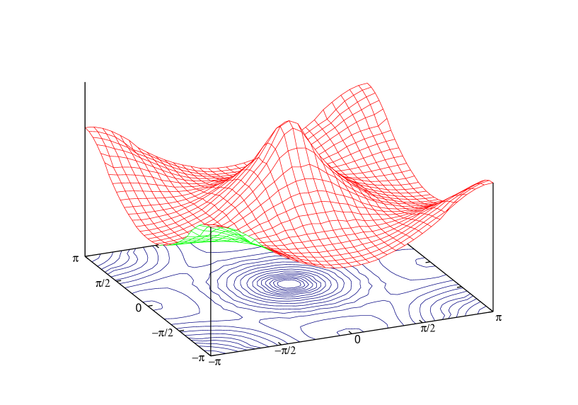
Figure 1: The dispersion relation $E(\vec{p})$ of a single electron in the $t$-$t^{\prime}$-$J$ model (on a $32\times 32$ lattice for $J=0.4t$ and $t^{\prime}=-0.3t$) with electron pockets centered at $(\frac{\pi}{a},0)$ and $(0,\frac{\pi}{a})$.

The location of these pockets again has important effects on the electron dynamics, which turns out to be quite different from that of the holes. In particular, in contrast to hole-doped systems, in electron-doped antiferromagnets the magnon-mediated forces between two electrons depend on the total momentum $\vec{P}$ of the pair. For $\vec{P}=0$ the one-magnon exchange potential between two electrons at distance $r$ is proportional to $1/r^{4}$, while in the hole case it has a $1/r^{2}$ dependence. The different locations of electron and hole pockets also affect the phase structure. While spiral phases are possible in the hole-doped case [5, 7, 52], they are absent in electron-doped cuprates [17, 20, 22, 24, 26].

The paper is organized as follows. In section 2 the symmetries of charge carrier fields are summarized. Based on this, the electron fields are identified and the hole fields are eliminated. The low-energy effective action for magnons and electrons is then constructed in a systematic manner. Section 3 contains the derivation of the one-magnon exchange potential between two electrons as well as a discussion of the corresponding Schrödinger equation. In section 4 spiral configurations of the staggered magnetization and in section 5 the reduction of the staggered magnetization upon doping are investigated. Section 6 contains our conclusions. The somewhat subtle transformation of the one-magnon exchange potential from momentum to coordinate space is discussed in an appendix.

2 Symmetries of Magnon and Electron Fields

In this section, based on [49, 51], we summarize the transformation properties of magnon and charge carrier fields. We then identify the electron fields and eliminate the hole fields in order to construct the low-energy effective theory for magnons and electrons.

2.1 Symmetries of Magnon Fields

In an antiferromagnet the spontaneous breaking of the $SU(2)_{s}$ spin symmetry down to $U(1)_{s}$ gives rise to two massless magnons. The staggered magnetization is described by a unit-vector field

$$\vec{e}(x)=(e_{1}(x),e_{2}(x),e_{3}(x))=(\sin\theta(x)\cos\varphi(x),\sin\theta(x)\sin\varphi(x),\cos\theta(x)),$$ (2.1)

in the coset space $SU(2)_{s}/U(1)_{s}=S^{2}$, where $x=(x_{1},x_{2},t)$ is a point in $(2+1)$-d space-time. It is convenient to use a ${\mathbb{C}}P(1)$ representation in terms of $2\times 2$ Hermitean projection matrices $P(x)$ with

$$P(x)=\frac{1}{2}({\mathbbm{1}}+\vec{e}(x)\cdot\vec{\sigma}),\quad P(x)^{\dagger}=P(x),\quad\mbox{Tr}P(x)=1,\quad P(x)^{2}=P(x).$$ (2.2)

As discussed in detail in [49], the magnon field transforms as

$$SU(2)_{s}: P(x)^{\prime} =gP(x)g^{\dagger},$$

$$SU(2)_{Q}: {}^{\vec{Q}}P(x) =P(x),$$

$$D_{i}: {}^{D_{i}}P(x) ={\mathbbm{1}}-P(x),$$

$$D^{\prime}_{i}: {}^{D^{\prime}_{i}}P(x) =P(x)^{*},$$

$$O: {}^{O}P(x) =P(Ox), \quad Ox =(-x_{2},x_{1},t),$$

$$R: {}^{R}P(x) =P(Rx), \quad Rx =(x_{1},-x_{2},t),$$

$$T: {}^{T}P(x) ={\mathbbm{1}}-P(Tx), \quad Tx =(x_{1},x_{2},-t),$$

$$T^{\prime}: {}^{T^{\prime}}P(x) =(i\sigma_{2})\left[{}^{T}P(x)\right](i\sigma_{2})^{\dagger}=P(Tx)^{*}.$$ (2.3)

The various symmetries are the $SU(2)_{s}$ spin rotations, the non-Abelian $SU(2)_{Q}$ extension of the $U(1)_{Q}$ fermion number symmetry (also known as pseudo-spin symmetry) that arises in the Hubbard model at half-filling, the displacement symmetry by one lattice spacing in the $i$-direction $D_{i}$, the symmetry $D_{i}$ combined with the spin rotation $i\sigma_{2}$ resulting in $D_{i}^{\prime}$, as well as the 90 degrees rotation $O$, the reflection at the $x_{1}$-axis $R$, time reversal $T$, and $T$ combined with the spin rotation $i\sigma_{2}$ resulting in $T^{\prime}$.

The spontaneously broken $SU(2)_{s}$ symmetry is nonlinearly realized on the charge carrier fields. The global $SU(2)_{s}$ symmetry then manifests itself as a local $U(1)_{s}$ symmetry in the unbroken subgroup, and the charge carrier fields couple to the magnon field via composite vector fields. In order to construct these vector fields one first diagonalizes $P(x)$ by a unitary transformation $u(x)\in SU(2)$, i.e.

$$u(x)P(x)u(x)^{\dagger}=\frac{1}{2}({\mathbbm{1}}+\sigma_{3})=\left(\begin{array}[]{cc}1&0\\ 0&0\end{array}\right),\qquad u_{11}(x)\geq 0,$$ (2.6)

$$u(x)=\left(\begin{array}[]{cc}\cos\frac{\theta(x)}{2}&\sin\frac{\theta(x)}{2}\exp(-i\varphi(x))\\ -\sin\frac{\theta(x)}{2}\exp(i\varphi(x))&\cos\frac{\theta(x)}{2}\end{array}\right).$$ (2.9)

Under a global $SU(2)_{s}$ transformation $g$, the diagonalizing field $u(x)$ transforms as

$$u(x)^{\prime}=h(x)u(x)g^{\dagger},\qquad u_{11}(x)^{\prime}\geq 0.$$ (2.10)

This defines the nonlinear symmetry transformation

$$h(x)=\exp(i\alpha(x)\sigma_{3})=\left(\begin{array}[]{cc}\exp(i\alpha(x))&0\\ 0&\exp(-i\alpha(x))\end{array}\right)\in U(1)_{s}.$$ (2.11)

Under the displacement symmetry $D_{i}$ the staggered magnetization changes sign, i.e. ${}^{D_{i}}\vec{e}(x)=-\vec{e}(x)$, and one obtains

$${}^{D_{i}}u(x)=\tau(x)u(x),\qquad\tau(x)=\left(\begin{array}[]{cc}0&-\exp(-i\varphi(x))\\ \exp(i\varphi(x))&0\end{array}\right).$$ (2.12)

In order to couple magnons and charge carriers, one constructs the traceless anti-Hermitean field

$$v_{\mu}(x)=u(x)\partial_{\mu}u(x)^{\dagger},$$ (2.13)

which transforms as

$$SU(2)_{s}: v_{\mu}(x)^{\prime} =h(x)[v_{\mu}(x)+\partial_{\mu}]h(x)^{\dagger},$$

$$SU(2)_{Q}: {}^{\vec{Q}}v_{\mu}(x) =v_{\mu}(x),$$

$$D_{i}: {}^{D_{i}}v_{\mu}(x) =\tau(x)[v_{\mu}(x)+\partial_{\mu}]\tau(x)^{\dagger},$$

$$D^{\prime}_{i}: {}^{D^{\prime}_{i}}v_{\mu}(x) =v_{\mu}(x)^{*},$$

$$O: {}^{O}v_{i}(x) =\varepsilon_{ij}v_{j}(Ox),\quad {}^{O}v_{t}(x) =v_{t}(Ox),$$

$$R: {}^{R}v_{1}(x) =v_{1}(Rx),\quad {}^{R}v_{2}(x) =-v_{2}(Rx),\quad^{R}v_{t}(x)=v_{t}(Rx),$$

$$T: {}^{T}v_{j}(x) =\ ^{D_{i}}v_{j}(Tx),\quad {}^{T}v_{t}(x) =-\ ^{D_{i}}v_{t}(Tx),$$

$$T^{\prime}: {}^{T^{\prime}}v_{j}(x) =\ ^{D^{\prime}_{i}}v_{j}(Tx),\quad {}^{T^{\prime}}v_{t}(x) =-^{D^{\prime}_{i}}v_{t}(Tx).$$ (2.14)

The field $v_{\mu}(x)$ decomposes into an Abelian “gauge” field $v_{\mu}^{3}(x)$ and two “charged” vector fields $v_{\mu}^{\pm}(x)$, i.e.

$$v_{\mu}(x)=iv_{\mu}^{a}(x)\sigma_{a},\qquad v_{\mu}^{\pm}(x)=v_{\mu}^{1}(x)\mp iv_{\mu}^{2}(x).$$ (2.15)

2.2 Fermion Fields in Momentum Space Pockets

In [51] matrix-valued charge carrier fields

$$\Psi^{k}(x)=\left(\begin{array}[]{cc}\psi^{k}_{+}(x)&\psi^{-k^{\prime}\dagger}_{-}(x)\\ \psi^{k}_{-}(x)&-\psi^{-k^{\prime}\dagger}_{+}(x)\end{array}\right),\quad\Psi^{k\dagger}(x)=\left(\begin{array}[]{cc}\psi^{k\dagger}_{+}(x)&\psi^{k\dagger}_{-}(x)\\ \psi^{-k^{\prime}}_{-}(x)&-\psi^{-k^{\prime}}_{+}(x)\end{array}\right)$$ (2.16)

have been constructed. Here $k^{\prime}=k+\big{(}\frac{\pi}{a},\frac{\pi}{a}\big{)}$ and $\psi^{k}_{\pm}(x)$ and $\psi^{k\dagger}_{\pm}(x)$ are independent Grassmann fields which are associated with the following eight lattice momentum values illustrated in figure 2

$$k=(k_{1},k_{2})\in\left\{\big{(}0,0\big{)},\;\big{(}\frac{\pi}{a},\frac{\pi}{a}\big{)},\;\big{(}\frac{\pi}{a},0\big{)},\;\big{(}0,\frac{\pi}{a}\big{)},\;\big{(}\pm\frac{\pi}{2a},\pm\frac{\pi}{2a}\big{)}\right\}.$$ (2.17)

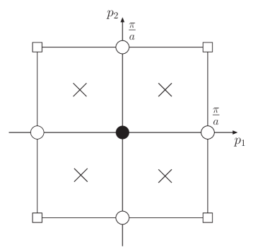
Figure 2: Eight lattice momenta and their periodic copies. In the cuprates the holes reside in momentum space pockets centered at lattice momenta $\big{(}\pm\frac{\pi}{2a},\pm\frac{\pi}{2a}\big{)}$ which are represented by the four crosses, while electrons reside at $\big{(}\frac{\pi}{a},0\big{)}$ or $\big{(}0,\frac{\pi}{a}\big{)}$ (represented by the circles).

The charge carrier fields transform as

$$SU(2)_{s}: \Psi^{k}(x)^{\prime} =h(x)\Psi^{k}(x),$$

$$SU(2)_{Q}: {}^{\vec{Q}}\Psi^{k}(x) =\Psi^{k}(x)\Omega^{T},$$

$$D_{i}: {}^{D_{i}}\Psi^{k}(x) =\exp(ik_{i}a)\tau(x)\Psi^{k}(x)\sigma_{3},$$

$$D^{\prime}_{i}: {}^{D^{\prime}_{i}}\Psi^{k}(x) =\exp(ik_{i}a)(i\sigma_{2})\Psi^{k}(x)\sigma_{3},$$

$$O: {}^{O}\Psi^{k}(x) =\Psi^{Ok}(Ox),$$

$$R: {}^{R}\Psi^{k}(x) =\Psi^{Rk}(Rx),$$

$$T: {}^{T}\Psi^{k}(x) =\tau(Tx)(i\sigma_{2})\left[\Psi^{-k\dagger}(Tx)^{T}\right]\sigma_{3},$$

$${}^{T}\Psi^{k\dagger}(x) =-\sigma_{3}\left[\Psi^{-k}(Tx)^{T}\right](i\sigma_{2})^{\dagger}\tau(Tx)^{\dagger},$$

$$T^{\prime}: {}^{T^{\prime}}\Psi^{k}(x) =-\left[\Psi^{-k\dagger}(Tx)^{T}\right]\sigma_{3},$$

$${}^{T^{\prime}}\Psi^{k\dagger}(x) =\sigma_{3}\left[\Psi^{-k}(Tx)^{T}\right].$$ (2.18)

Here $\Omega\in SU(2)_{Q}$ and $Ok$ and $Rk$ are the momenta obtained by rotating or reflecting the momentum $k$.

2.3 Electron Field Identification and Hole Field Elimination

ARPES measurements as well as theoretical investigations [27, 28, 29, 30, 31, 32, 33] (see also figure 1) indicate that electrons doped into an antiferromagnet appear in momentum space pockets centered at

$$k=\big{(}\frac{\pi}{a},0\big{)},\qquad k^{\prime}=\big{(}0,\frac{\pi}{a}\big{)}.$$ (2.19)

Hence, only the fermion fields with these two momentum labels will appear in the low-energy effective theory. Using the transformation rules of eq.(2.2) one can construct the following invariant mass terms

$$\frac{1}{2}\mbox{Tr}\big{[}{\cal M}(\Psi^{k\dagger}\sigma_{3} \Psi^{k^{\prime}}+\Psi^{k^{\prime}\dagger}\sigma_{3}\Psi^{k})+m(\Psi^{k\dagger}\Psi^{k}\sigma_{3}+\Psi^{k^{\prime}\dagger}\Psi^{k^{\prime}}\sigma_{3})\big{]}$$

$$= \;\;\;{\cal M}\big{(}\psi^{k\dagger}_{+}\psi^{k^{\prime}}_{+}-\psi^{k\dagger}_{-}\psi^{k^{\prime}}_{-}+\psi^{k^{\prime}\dagger}_{+}\psi^{k}_{+}-\psi^{k^{\prime}\dagger}_{-}\psi^{k}_{-}\big{)}$$

$$+m\big{(}\psi^{k\dagger}_{+}\psi^{k}_{+}+\psi^{k\dagger}_{-}\psi^{k}_{-}+\psi^{k^{\prime}\dagger}_{+}\psi^{k^{\prime}}_{+}+\psi^{k^{\prime}\dagger}_{-}\psi^{k^{\prime}}_{-}\big{)}$$

$$= \;\;\;\big{(}\psi^{k\dagger}_{+},\,\psi^{k^{\prime}\dagger}_{+}\big{)}\bigg{(}\begin{array}[]{cc}m&{\cal M}\\ {\cal M}&m\end{array}\bigg{)}\bigg{(}\begin{array}[]{c}\psi^{k}_{+}\\ \psi^{k^{\prime}}_{+}\end{array}\bigg{)}$$ (2.24)

$$+\big{(}\psi^{k\dagger}_{-},\,\psi^{k^{\prime}\dagger}_{-}\big{)}\bigg{(}\begin{array}[]{cc}m&-{\cal M}\\ -{\cal M}&m\end{array}\bigg{)}\bigg{(}\begin{array}[]{c}\psi^{k}_{-}\\ \psi^{k^{\prime}}_{-}\end{array}\bigg{)}.$$ (2.29)

The terms proportional to ${\cal M}$ are $SU(2)_{Q}$-invariant while those proportional to $m$ are only $U(1)_{Q}$-invariant. By diagonalizing the mass matrices, electron and hole fields can be identified. The resulting eigenvalues are $m\pm{\cal M}$. In the $SU(2)_{Q}$-symmetric case, i.e. for $m=0$, there is an electron-hole symmetry. The electrons correspond to positive energy states with eigenvalue ${\cal M}$ and the holes correspond to negative energy states with eigenvalue $-{\cal M}$. In the presence of $SU(2)_{Q}$-breaking terms these energies are shifted and electrons now correspond to states with eigenvalue $m+{\cal M}$, while holes correspond to states with eigenvalue $m-{\cal M}$. The electron fields are given by the corresponding eigenvectors

$$\psi_{+}(x)=\frac{1}{\sqrt{2}}\big{[}\psi^{k}_{+}(x)+\psi^{k^{\prime}}_{+}(x)\big{]},\qquad\psi_{-}(x)=\frac{1}{\sqrt{2}}\big{[}\psi^{k}_{-}(x)-\psi^{k^{\prime}}_{-}(x)\big{]}.$$ (2.30)

Under the various symmetries they transform as

$$SU(2)_{s}: \psi_{\pm}(x)^{\prime} =\exp(\pm i\alpha(x))\psi_{\pm}(x),$$

$$U(1)_{Q}: {}^{Q}\psi_{\pm}(x) =\exp(i\omega)\psi_{\pm}(x),$$

$$D_{i}: {}^{D_{i}}\psi_{\pm}(x) =\mp\exp(ik_{i}a)\exp(\mp i\varphi(x))\psi_{\mp}(x),$$

$$D^{\prime}_{i}: {}^{D^{\prime}_{i}}\psi_{\pm}(x) =\pm\exp(ik_{i}a)\psi_{\mp}(x),$$

$$O: {}^{O}\psi_{\pm}(x) =\pm\psi_{\pm}(Ox),$$

$$R: {}^{R}\psi_{\pm}(x) =\psi_{\pm}(Rx),$$

$$T: {}^{T}\psi_{\pm}(x) =\exp(\mp i\varphi(Tx))\psi^{\dagger}_{\pm}(Tx),$$

$${}^{T}\psi^{\dagger}_{\pm}(x) =-\exp(\pm i\varphi(Tx))\psi_{\pm}(Tx),$$

$$T^{\prime}: {}^{T^{\prime}}\psi_{\pm}(x) =-\psi^{\dagger}_{\pm}(Tx),$$

$${}^{T^{\prime}}\psi^{\dagger}_{\pm}(x) =\psi_{\pm}(Tx).$$ (2.31)

The action of magnons and electrons must be invariant under these symmetries.

2.4 Effective Action for Magnons and Electrons

We decompose the action into terms containing different numbers of fermion fields $n_{\psi}$ (with $n_{\psi}$ even) such that

$$S[\psi^{\dagger}_{\pm},\psi_{\pm},P]=\int d^{2}x\ dt\ \sum_{n_{\psi}}{\cal L}_{n_{\psi}}.$$ (2.32)

The leading terms in the effective Lagrangian without fermion fields are given by

$${\cal L}_{0}=\rho_{s}\mbox{Tr}\big{[}\partial_{i}P\partial_{i}P+\frac{1}{c^{2}}\partial_{t}P\partial_{t}P\big{]},$$ (2.33)

with the spin stiffness $\rho_{s}$ and the spinwave velocity $c$ as low-energy parameters. The terms with two fermion fields (containing at most one temporal or two spatial derivatives) describe the propagation of electrons as well as their couplings to magnons, and are given by

$${\cal L}_{2}= \sum_{s=+,-}\Big{[}M\psi^{\dagger}_{s}\psi_{s}+\psi^{\dagger}_{s}D_{t}\psi_{s}+\frac{1}{2M^{\prime}}D_{i}\psi^{\dagger}_{s}D_{i}\psi_{s}+N\psi^{\dagger}_{s}v^{s}_{i}v^{-s}_{i}\psi_{s}$$

$$\hskip 18.00005pt+iK\big{(}D_{1}\psi^{\dagger}_{s}v^{s}_{1}\psi_{-s}-\psi^{\dagger}_{s}v^{s}_{1}D_{1}\psi_{-s}-D_{2}\psi^{\dagger}_{s}v^{s}_{2}\psi_{-s}+\psi^{\dagger}_{s}v^{s}_{2}D_{2}\psi_{-s}\big{)}\Big{]}.$$ (2.34)

Here $M$ is the rest mass and $M^{\prime}$ is the kinetic mass of an electron, $K$ is an electron-one-magnon, and $N$ is an electron-two-magnon coupling, which all take real values. The covariant derivatives are given by

$$D_{t}\psi_{\pm}(x) =\left[\partial_{t}\pm iv_{t}^{3}(x)-\mu\right]\psi_{\pm}(x),$$

$$D_{i}\psi_{\pm}(x) =\left[\partial_{i}\pm iv_{i}^{3}(x)\right]\psi_{\pm}(x).$$ (2.35)

The chemical potential $\mu$ enters the covariant time-derivative like an imaginary constant vector potential for the fermion number symmetry $U(1)_{Q}$.

Next we list the contributions with four fermion fields including up to one temporal or two spatial derivatives

$${\cal L}_{4}= \sum_{s=+,-}\Big{[}\frac{G_{1}}{2}\psi^{\dagger}_{s}\psi_{s}\psi^{\dagger}_{-s}\psi_{-s}+G_{2}D_{i}\psi^{\dagger}_{s}D_{i}\psi_{s}\psi^{\dagger}_{s}\psi_{s}+G_{3}D_{i}\psi^{\dagger}_{s}D_{i}\psi_{s}\psi^{\dagger}_{-s}\psi_{-s}$$

$$\hskip 18.99995pt+G_{4}D_{i}\psi^{\dagger}_{s}D_{i}\psi_{-s}\psi^{\dagger}_{-s}\psi_{s}+\frac{G_{5}}{2}\big{(}D_{i}\psi^{\dagger}_{s}\psi_{s}D_{i}\psi^{\dagger}_{-s}\psi_{-s}+\psi^{\dagger}_{s}D_{i}\psi_{s}\psi^{\dagger}_{-s}D_{i}\psi_{-s}\big{)}$$

$$\hskip 18.99995pt+iG_{6}\big{(}D_{1}\psi^{\dagger}_{s}\psi_{s}\psi^{\dagger}_{s}v^{s}_{1}\psi_{-s}-\psi^{\dagger}_{s}D_{1}\psi_{s}\psi^{\dagger}_{-s}v^{-s}_{1}\psi_{s}$$

$$\hskip 38.00008pt-D_{2}\psi^{\dagger}_{s}\psi_{s}\psi^{\dagger}_{s}v^{s}_{2}\psi_{-s}+\psi^{\dagger}_{s}D_{2}\psi_{s}\psi^{\dagger}_{-s}v^{-s}_{2}\psi_{s}\big{)}+\frac{G_{7}}{2}\psi^{\dagger}_{s}\psi_{s}v^{s}_{i}v^{-s}_{i}\psi^{\dagger}_{-s}\psi_{-s}$$

$$\hskip 18.99995pt+\frac{G_{8}}{2}\big{(}D_{t}\psi^{\dagger}_{s}\psi_{s}\psi^{\dagger}_{-s}\psi_{-s}-\psi^{\dagger}_{s}D_{t}\psi_{s}\psi^{\dagger}_{-s}\psi_{-s}\big{)}\Big{]}.$$ (2.36)

Since it contains $D_{t}$, the term proportional to $G_{8}$ would imply a deviation from canonical anticommutation relations in a Hamiltonian formulation of the theory. Fortunately, this term can be eliminated by a field redefinition $\psi_{s}\rightarrow\psi_{s}+\frac{G_{8}}{2}\psi_{s}\psi_{-s}^{\dagger}\psi_{-s}$. The redefined field obeys the same symmetry transformations as the original one and is constructed such that after the field redefinition $G_{8}=0$. All other terms in the action are reproduced in their present form.

For completeness, we finally list the only contribution with more than four fermion fields, again including up to one temporal or two spatial derivatives

$${\cal L}_{6}=\sum_{s=+,-} HD_{i}\psi^{\dagger}_{s}D_{i}\psi_{s}\psi^{\dagger}_{s}\psi_{s}\psi^{\dagger}_{-s}\psi_{-s}.$$ (2.37)

The leading fermion contact term is proportional to $G_{1}$. Due to the large number of low-energy parameters $G_{2},...,G_{7},H$, the higher-order terms are unlikely to be used in practical applications. We have used the algebraic program FORM [53], and independently thereof, the GiNaC framework for symbolic computation within the C++ programming language [54], to verify that the terms listed above form a complete linearly independent set.

It should be noted that, unlike in the hole case, the leading terms in the effective action are not invariant against Galilean boosts. This is not unexpected because the underlying microscopic systems also lack this symmetry. The lack of Galilean boost invariance has important physical consequences. In particular, the magnon-mediated forces between two electrons will turn out to depend on the total momentum $\vec{P}$ of the pair. Thus it is not sufficient to consider the two particles in their rest frame, i.e. at $\vec{P}=0$. This is due to the underlying crystal lattice which defines a preferred rest-frame (a condensed matter “ether”).

3 Magnon-mediated Binding between Electrons

We treat the forces between two electrons in the same way as the ones in the effective theory for magnons and holes [50, 51]. As in that case, one-magnon exchange dominates the long-range forces. In this section we calculate the one-magnon exchange potential between two electrons and we solve the corresponding two-particle Schrödinger equation.

3.1 One-Magnon Exchange Potential between Electrons

In order to calculate the one-magnon exchange potential between two electrons, we expand in the magnon fluctuations $m_{1}(x)$, $m_{2}(x)$ around the ordered staggered magnetization, i.e.

$$\vec{e}(x)=\Big{(}\frac{m_{1}(x)}{\sqrt{\rho_{s}}},\, \frac{m_{2}(x)}{\sqrt{\rho_{s}}},1\Big{)}+{\cal O}(m^{2})$$

$$\Rightarrow\quad v_{\mu}^{\pm}(x) =\frac{1}{2\sqrt{\rho_{s}}}\partial_{\mu}\big{[}m_{2}(x)\pm im_{1}(x)\big{]}+{\cal O}(m^{3}),$$

$$v_{\mu}^{3}(x) =\frac{1}{4\rho_{s}}\big{[}m_{1}(x)\partial_{\mu}m_{2}(x)-m_{2}(x)\partial_{\mu}m_{1}(x)\big{]}+{\cal O}(m^{4}).$$ (3.1)

The vertices with $v_{\mu}^{3}(x)$ (contained in $D_{\mu}$) involve at least two magnon fields. Hence, one-magnon exchange results exclusively from vertices with $v_{\mu}^{\pm}(x)$. Thus, two electrons can exchange a single magnon only if they have antiparallel spins ($+$ and $-$), which are both flipped in the magnon exchange process. We denote the momenta of the incoming and outgoing electrons by $\vec{p}_{\pm}$ and $\vec{p}_{\pm}\ \!\!\!\!^{\prime}\$, respectively. Furthermore, $\vec{q}$ represents the momentum of the exchanged magnon. We also introduce the total momentum $\vec{P}$ as well as the incoming and outgoing relative momenta $\vec{p}$ and $\vec{p}\ ^{\prime}$

$$\vec{P}=\vec{p}_{+}+\vec{p}_{-}=\vec{p}_{+}\ \!\!\!\!^{\prime}+\vec{p}_{-}\ \!\!\!\!^{\prime}\>,$$

$$\vec{p}=\frac{1}{2}(\vec{p}_{+}-\vec{p}_{-}),\qquad\vec{p}\ ^{\prime}=\frac{1}{2}(\vec{p}_{+}\ \!\!\!\!^{\prime}-\vec{p}_{-}\ \!\!\!\!^{\prime}).$$ (3.2)

Due to momentum conservation we then have

$$\vec{q}=\vec{p}+\vec{p}\ ^{\prime}.$$ (3.3)

Figure 3 shows the Feynman diagram describing one-magnon exchange.

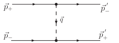
Figure 3: Feynman diagram for one-magnon exchange between two electrons with antiparallel spins undergoing a spin-flip.

In momentum space the resulting one-magnon exchange potential takes the form

$$\langle\vec{p}_{+}\ \!\!\!\!^{\prime}\ \vec{p}_{-}\ \!\!\!\!^{\prime}|V|\vec{p}_{+}\vec{p}_{-}\rangle =\frac{K^{2}}{2\rho_{s}}\frac{1}{q^{2}}\left[q_{1}^{2}-q_{2}^{2}+2(q_{1}p_{-1}-q_{2}p_{-2})\right]\left[q_{1}^{2}-q_{2}^{2}-2(q_{1}p_{+1}-q_{2}p_{+2})\right]$$

$$\;\;\;\;\times\delta(\vec{p}_{+}+\vec{p}_{-}-\vec{p}_{+}\ \!\!\!\!^{\prime}-\vec{p}_{-}\ \!\!\!\!^{\prime}).$$ (3.4)

Transforming the potential to coordinate space is not entirely trivial and is thus discussed in the appendix. In coordinate space the resulting potential is given by

$$\langle\vec{r}_{+}\ \!\!\!\!^{\prime}\vec{r}_{-}\ \!\!\!\!^{\prime}|V|\vec{r}_{+}\vec{r}_{-}\rangle=\frac{K^{2}}{2\pi\rho_{s}}\left[12\frac{\cos(4\varphi)}{r^{4}}+\frac{P^{2}}{2}\frac{\cos(2(\varphi+\chi))}{r^{2}}\right]\delta(\vec{r}_{+}-\vec{r}_{-}\ \!\!\!\!^{\prime})\ \delta(\vec{r}_{-}-\vec{r}_{+}\ \!\!\!\!^{\prime}).$$ (3.5)

Here $\varphi$ is the angle between the distance vector $\vec{r}=\vec{r}_{+}-\vec{r}_{-}$ of the two electrons and the $x_{1}$-axis. In contrast to the hole case, the potential depends on the magnitude $P$ of the total momentum $\vec{P}$ as well as on the angle $\chi$ between $\vec{P}$ and the $x_{1}$-axis. For $\vec{P}=0$ the one-magnon exchange potential between two electrons falls off as $1/r^{4}$, while in the hole case it is proportional to $1/r^{2}$. Retardation effects enter at higher orders only and thus the potential is instantaneous. We have omitted short-distance $\delta$-function contributions to the potential which add to the 4-fermion contact interactions. Since we will model the short-distance repulsion by a hard-core radius, the $\delta$-function contributions will not be needed in the following.

3.2 Schrödinger Equation for two Electrons

Let us consider two electrons with opposite spins $+$ and $-$. The wave function depends on the relative distance vector $\vec{r}$ which points from the spin $-$ electron to the spin $+$ electron. Magnon exchange is accompanied by a spin-flip. Hence, the vector $\vec{r}$ changes its direction in the magnon exchange process. The resulting Schrödinger equation then takes the form

$$-\frac{1}{M^{\prime}}\Delta\Psi(\vec{r})+\frac{K^{2}}{2\pi\rho_{s}}\left[12\frac{\cos(4\varphi)}{r^{4}}+\frac{P^{2}}{2}\frac{\cos(2(\varphi+\chi))}{r^{2}}\right]\Psi(-\vec{r})=\bigg{[}E-\frac{P^{2}}{2M^{\prime}}\bigg{]}\Psi(\vec{r}).$$ (3.6)

For simplicity, instead of explicitly using the 4-fermion contact interactions, we model the short-distance repulsion between the electrons by a hard-core of radius $r_{0}$, i.e. we require $\Psi(\vec{r})=0$ for $|\vec{r}|\leq r_{0}$. In contrast to the hole case [50, 51], we have not been able to solve the above Schrödinger equation analytically. Instead, we have solved it numerically. A typical probability distribution for the ground state is illustrated in figure 4 for $\vec{P}=0$.

Figure 4: Probability distribution for the ground state of two electrons with total momentum $\vec{P}=(0,0)$.

The probability distribution resembles $d_{xy}$ symmetry. However, due to the 90 degrees rotation symmetry the continuum classification scheme of angular momenta is inappropriate. Under the group of discrete rotations and reflections the ground state wave function transforms in the trivial representation.

Due to the lack of Galilean boost invariance, the two-electron bound state changes its structure when it is boosted out of its rest frame. Of course, an electron pair with total momentum $\vec{P}\neq 0$ costs additional kinetic energy $P^{2}/2M^{\prime}$ for the center of mass motion. In addition, the binding energy also depends on $\vec{P}$. The strongest binding arises when the total momentum $\vec{P}$ points along a lattice diagonal. The corresponding probability distribution is illustrated in figure 5.

Figure 5: Probability distribution for the ground state of two electrons with total momentum $\vec{P}=\frac{1}{\sqrt{2}}(P,P)$ along a lattice diagonal.

Since they depend crucially on the precise values of the low-energy parameters, we have not attempted an extensive numerical investigation of the binding energy and other properties of the two-electron bound states. Once the low-energy parameters have been determined for a concrete underlying microscopic system, a precise calculation of the physical properties of the two-electron bound state is straightforward using the numerical method employed above.

In order to gain at least some approximate analytic insight into the bound state problem, let us also consider the semi-classical Bohr-Sommerfeld quantization. First, we consider a pair of electrons with total momentum $\vec{P}=0$ moving relative to each other along a lattice diagonal. The classical energy of the periodic relative motion is given by

$$E=M^{\prime}\left(\frac{dr}{dt}\right)^{2}-\frac{6K^{2}}{\pi\rho_{s}r^{4}}.$$ (3.7)

The Bohr-Sommerfeld quantization condition implies

$$S+ET = \int_{0}^{T}dt\ \left[M^{\prime}\left(\frac{dr}{dt}\right)^{2}+\frac{6K^{2}}{\pi\rho_{s}r^{4}}+E\right]=2\int_{0}^{T}dt\ M^{\prime}\left(\frac{dr}{dt}\right)^{2}$$ (3.8)

$$= 4\int_{r_{0}}^{R}dr\ M^{\prime}\ \frac{dr}{dt}=4\int_{r_{0}}^{R}dr\ \sqrt{EM^{\prime}+\frac{6K^{2}M^{\prime}}{\pi\rho_{s}r^{4}}}=2\pi n,$$

where $S$ is the action, $T$ is the period of the motion, and $n$ is a positive integer. The hard-core radius $r_{0}$ is a classical turning point and $R$ is the other classical turning point determined by

$$E=-\frac{6K^{2}}{\pi\rho_{s}R^{4}}.$$ (3.9)

The above equations lead to a relatively complicated expression for the energy in terms of elliptic integrals. Instead of investigating these expressions, we limit ourselves to estimating the number of bound states. For this purpose, we set $E=0$ which implies $R=\infty$, and we then obtain

$$n=\left[\ \int_{r_{0}}^{\infty}dr\ \sqrt{\frac{24K^{2}M^{\prime}}{\pi^{3}\rho_{s}r^{4}}}\ \right]=\left[\ \sqrt{\frac{24K^{2}M^{\prime}}{\pi^{3}\rho_{s}r_{0}^{2}}}\ \right].$$ (3.10)

The brackets denote the nearest integer smaller than the expression enclosed in the brackets. In particular, Bohr-Sommerfeld quantization suggests that a bound state exists only if

$$\frac{24K^{2}M^{\prime}}{\pi^{3}\rho_{s}r_{0}^{2}}\geq 1.$$ (3.11)

Of course, one should be aware of the fact that this is at best a semi-quantitative estimate because Bohr-Sommerfeld quantization should not be trusted quantitatively for small quantum numbers. Let us also repeat these considerations for $\vec{P}\neq 0$. Again, we consider $\vec{P}=\frac{1}{\sqrt{2}}(P,P)$ such that the diagonal motion of an electron-pair has the energy

$$E=M^{\prime}\left(\frac{dr}{dt}\right)^{2}-\frac{K^{2}}{2\pi\rho_{s}}\left(\frac{12}{r^{4}}+\frac{P^{2}}{2r^{2}}\right).$$ (3.12)

In complete analogy to the $\vec{P}=0$ case one then obtains

$$n=\left[\ \int_{r_{0}}^{\infty}dr\ \sqrt{\frac{2K^{2}M^{\prime}}{\pi^{3}\rho_{s}}\left(\frac{12}{r^{4}}+\frac{P^{2}}{2r^{2}}\right)}\ \right]\rightarrow\infty,$$ (3.13)

which suggests that infinitely many two-electron bound states exist for $\vec{P}\neq 0$. This is similar to the two-hole problem which has a $1/r^{2}$ potential with infinitely many bound states already for $\vec{P}=0$ [50, 51].

Two-electron bound states with $\vec{P}=0$ have been considered before by Kuchiev and Sushkov [19] in the context of the $t$-$t^{\prime}$-$J$ model. In contrast to the hole-case [13] with a $1/r^{2}$ potential and an infinite number of bound states, in the electron-case only a finite number of bound states was found. While some results of that work agree qualitatively with the results of our effective theory, there are also important differences. For example, in [19] the magnon-electron vertex was considered to be the same as the magnon-hole vertex, while the two vertices are different in the effective theory.

4 Investigation of Spiral Phases

In the following we will investigate phases with constant fermion density. The most general magnon field configuration $\vec{e}(x)$ which provides a constant background field for the doped electrons is not necessarily constant itself, but may represent a spiral in the staggered magnetization. While a spiral costs magnetic energy proportional to the spin stiffness $\rho_{s}$, the electrons might lower their energy by propagating in the spiral background. However, we will find that spiral phases are not energetically favorable in electron-doped systems.

4.1 Spirals with Uniform Composite Vector Fields

Since the electrons couple to the composite vector field $v_{i}(x)$ in a gauge covariant way, in order to provide a constant background field for the electrons, $v_{i}(x)$ must be constant up to a gauge transformation, i.e.

$${v^{3}_{i}}(x)^{\prime} =v^{3}_{i}(x)-\partial_{i}\alpha(x)=\partial_{i}\varphi(x)\sin^{2}\frac{\theta(x)}{2}-\partial_{i}\alpha(x)=c^{3}_{i},$$

$${v^{\pm}_{i}}(x)^{\prime} =v^{\pm}_{i}(x)\exp\big{(}\pm 2i\alpha(x)\big{)}$$

$$=\frac{1}{2}\big{[}\partial_{i}\varphi(x)\sin\theta(x)\pm i\partial_{i}\theta(x)\big{]}\exp\big{(}\pm 2i\alpha(x)\mp i\varphi(x)\big{)}=c^{\pm}_{i},$$ (4.1)

with $c^{3}_{i}$ and $c^{\pm}_{i}$ being constant. As shown in [52], the most general configuration that leads to a constant $v_{i}(x)^{\prime}$ represents a spiral in the staggered magnetization. In addition, by an appropriate gauge transformation one can always put

$$c_{i}^{+}=c_{i}^{-}=c_{i}\in{\mathbb{R}}.$$ (4.2)

The magnetic energy density of such configurations takes the form

$$\epsilon_{m}=\frac{\rho_{s}}{2}\partial_{i}\vec{e}(x)\cdot\partial_{i}\vec{e}(x)=2\rho_{s}v_{i}^{+}(x)v_{i}^{-}(x)=2\rho_{s}c_{i}c_{i}.$$ (4.3)

We now consider a concrete family of spiral configurations with

$$\theta(x)=\theta_{0},\qquad\quad\varphi(x)=k_{i}x_{i},$$ (4.4)

which implies

$$v_{t}(x)=0,\qquad v^{3}_{i}(x)=k_{i}\sin^{2}\frac{\theta_{0}}{2},\qquad v_{i}^{\pm}(x)=\frac{k_{i}}{2}\sin\theta_{0}\exp(\mp ik_{i}x_{i}).$$ (4.5)

Performing the gauge transformation

$$\alpha(x)=\frac{1}{2}k_{i}x_{i},$$ (4.6)

one arrives at

$$v_{t}(x)^{\prime} =v_{t}(x)-\partial_{t}\alpha(x)=0,$$

$${v^{3}_{i}}(x)^{\prime} =v^{3}_{i}(x)-\partial_{i}\alpha(x)=k_{i}\bigg{[}\sin^{2}\frac{\theta_{0}}{2}-\frac{1}{2}\bigg{]}=c^{3}_{i},$$

$${v^{\pm}_{i}}(x)^{\prime} =v^{\pm}_{i}(x)\exp\big{(}\pm 2i\alpha(x)\big{)}=\frac{k_{i}}{2}\sin\theta_{0}=c_{i},$$ (4.7)

such that

$$c^{3}_{i}=-\frac{k_{i}}{2}\cos\theta_{0},\qquad\quad a=\frac{|c_{i}|}{c^{3}_{i}}=-\tan\theta_{0}.$$ (4.8)

The magnetic energy density then takes the form

$$\epsilon_{m}=2\rho_{s}c_{i}c_{i}=\frac{\rho_{s}}{2}\big{(}k_{1}^{2}+k_{2}^{2}\big{)}\sin^{2}\theta_{0}.$$ (4.9)

4.2 Fermionic Contributions to the Energy

Let us now compute the fermionic contribution to the energy, first keeping the parameters $c^{3}_{i}$ and $c_{i}$ of the spiral fixed, and neglecting the 4-fermion contact interactions. The Euclidean action of eq.(2.4) implies the following fermion Hamiltonian

$$H= \sum_{s=+,-}\Big{[}M\Psi^{\dagger}_{s}\Psi_{s}+\frac{1}{2M^{\prime}}D_{i}\Psi^{\dagger}_{s}D_{i}\Psi_{s}+N\Psi^{\dagger}_{s}v^{s}_{i}v^{-s}_{i}\Psi_{s}$$

$$\hskip 18.00005pt+iK\big{(}D_{1}\Psi^{\dagger}_{s}v^{s}_{1}\Psi_{-s}-\Psi^{\dagger}_{s}v^{s}_{1}D_{1}\Psi_{-s}-D_{2}\Psi^{\dagger}_{s}v^{s}_{2}\Psi_{-s}+\Psi^{\dagger}_{s}v^{s}_{2}D_{2}\Psi_{-s}\big{)}\Big{]},$$ (4.10)

with the covariant derivative

$$D_{i}\Psi_{\pm}(x)=[\partial_{i}\pm iv^{3}_{i}(x)]\Psi_{\pm}(x).$$ (4.11)

Here $\Psi^{\dagger}_{\pm}(x)$ and $\Psi_{\pm}(x)$ are creation and annihilation operators (not Grassmann numbers) for electrons with spin parallel ($+$) or antiparallel ($-$) to the local staggered magnetization. The Hamiltonian is invariant under time-independent $U(1)_{s}$ gauge transformations

$$\Psi_{\pm}(x)^{\prime} =\exp\big{(}\pm i\alpha(x)\big{)}\Psi_{\pm}(x),$$

$${v^{3}_{i}}(x)^{\prime} =v^{3}_{i}(x)-\partial_{i}\alpha(x),$$

$${v^{\pm}_{i}}(x)^{\prime} =v^{\pm}_{i}(x)\exp\big{(}\pm 2i\alpha(x)\big{)}.$$ (4.12)

We now consider electrons propagating in the background of a spiral in the staggered magnetization with

$${v^{3}_{i}}(x)^{\prime}=c^{3}_{i},\qquad\quad{v^{\pm}_{i}}(x)^{\prime}=c_{i}\in{\mathbb{R}}.$$ (4.13)

After an appropriate gauge transformation, the fermions propagate in a constant composite vector field ${v_{i}}(x)^{\prime}$. The Hamiltonian is diagonalized by going to momentum space. The Hamiltonian for single electrons with spatial momentum $\vec{p}=(p_{1},p_{2})$ is given by

$$H(\vec{p})=\left(\begin{array}[]{cc}M+\frac{(p_{i}-c_{i}^{3})^{2}}{2M^{\prime}}+Nc_{i}c_{i}&2K(-p_{1}c_{1}+p_{2}c_{2})\\ 2K(-p_{1}c_{1}+p_{2}c_{2})&M+\frac{(p_{i}+c_{i}^{3})^{2}}{2M^{\prime}}+Nc_{i}c_{i}\end{array}\right).$$ (4.14)

The diagonalization of the Hamiltonian yields

$$E_{\pm}(\vec{p})=M+\frac{p_{i}^{2}+(c_{i}^{3})^{2}}{2M^{\prime}}+Nc_{i}c_{i}\pm\sqrt{\bigg{(}\frac{p_{i}c_{i}^{3}}{M^{\prime}}\bigg{)}^{2}+4K^{2}(p_{1}c_{1}-p_{2}c_{2})^{2}}.$$ (4.15)

It should be noted that in this case the index $\pm$ does not refer to the spin orientation. In fact, the eigenvectors corresponding to $E_{\pm}(\vec{p})$ are linear combinations of both spins. Since $c_{i}^{3}$ does not affect the magnetic contribution to the energy density, it can be fixed by minimizing $E_{\pm}(\vec{p})$ which leads to $c_{1}^{3}=c_{2}^{3}=0$. According to eq.(4.1) this implies that $\theta_{0}=\frac{\pi}{2}$, i.e. the spiral is along a great circle on the sphere $S^{2}$. For $c_{i}^{3}=0$ the energies of eq.(4.15) reduce to

$$E_{\pm}(\vec{p})=M+\frac{p_{i}^{2}}{2M^{\prime}}+Nc_{i}c_{i}\pm 2K|p_{1}c_{1}-p_{2}c_{2}|.$$ (4.16)

The lines of constant energy are shown in figure 6. In particular, the lines of constant $E_{-}(\vec{p})$ are circles centered around $\pm 2KM^{\prime}(c_{1},-c_{2})$.

Figure 6: Lines of constant energy for electrons propagating in a spiral configuration. The contours of the lower energy $E_{-}(\vec{p})$ are shown on the left, and the contours of the higher energy $E_{+}(\vec{p})$ are displayed on the right.

For given $c_{i}\neq 0$ we now fill the lowest energy states with a small number of electrons. The filled electron pockets are circles centered around $\pm 2KM^{\prime}(c_{1},-c_{2})$ with a radius determined by the kinetic energy

$$T=\frac{1}{2M^{\prime}}\left[(p_{1}\mp 2KM^{\prime}c_{1})^{2}+(p_{2}\pm 2KM^{\prime}c_{2})^{2}\right]$$ (4.17)

of an electron at the Fermi surface. The two occupied circular electron pockets define a region $P$ in momentum space. The area of this region determines the fermion density as

$$n=\frac{1}{(2\pi)^{2}}\int_{P}d^{2}p=\frac{1}{\pi}M^{\prime}T.$$ (4.18)

The two circles do not overlap as long as $n<\frac{2}{\pi}M^{\prime 2}K^{2}c_{i}c_{i}$. The kinetic energy density of the filled region $P$ is given by

$$t=\frac{1}{(2\pi)^{2}}\int_{P}d^{2}p\ \frac{1}{2M^{\prime}}\left[(p_{1}\mp 2KM^{\prime}c_{1})^{2}+(p_{2}\pm 2KM^{\prime}c_{2})^{2}\right]=\frac{1}{2\pi}M^{\prime}T^{2}=\frac{\pi n^{2}}{2M^{\prime}},$$ (4.19)

and the total energy density of electrons then is

$$\epsilon_{e}=(M+Nc_{i}c_{i}-2K^{2}M^{\prime}c_{i}c_{i})n+\frac{\pi n^{2}}{2M^{\prime}}.$$ (4.20)

The resulting total energy density that includes the vacuum energy density $\epsilon_{0}$ as well as the magnetic energy density $\epsilon_{m}$ is given by

$$\epsilon=\epsilon_{0}+\epsilon_{m}+\epsilon_{e}=\epsilon_{0}+2\rho_{s}c_{i}c_{i}+(M+Nc_{i}c_{i}-2K^{2}M^{\prime}c_{i}c_{i})n+\frac{\pi n^{2}}{2M^{\prime}}.$$ (4.21)

For $\rho_{s}>(K^{2}M^{\prime}-\frac{1}{2}N)n$ (which is always satisfied for sufficiently small density $n$) the energy is minimized for $c_{i}=0$ and the value of the energy density at the minimum is given by

$$\epsilon=\epsilon_{0}+Mn+\frac{\pi n^{2}}{2M^{\prime}}.$$ (4.22)

However, one should not forget that, as the $c_{i}$ become smaller, the two occupied circles eventually touch each other once $\frac{2}{\pi}M^{\prime 2}K^{2}c_{i}c_{i}=n$. Interestingly, in this moment the states with energy $E_{+}(\vec{p})$ also become occupied. Indeed, as one can see in figure 6, the almond-shaped region of occupied states with energy $E_{+}(\vec{p})$ and the peanut-shaped region of occupied states with energy $E_{-}(\vec{p})$, combine to two complete overlapping circles. This is also illustrated in figure 7, in which the energies $E_{-}(\vec{p})$ and $E_{+}(\vec{p})$ combine to form two overlapping parabolic dispersion relations.

Figure 7: The energies $E_{-}(\vec{p})$ (solid curve) and $E_{+}(\vec{p})$ (dashed curve) along the line $\vec{p}\propto(c_{1},-c_{2})$ (the dashed lines in figure 6) define two independent parabolic dispersion relations.

As a result, eq.(4.22) is still valid even when the occupied circles overlap. Consequently, the energy minimum is indeed at $c_{i}=0$ and thus a homogeneous phase arises. This is in contrast to hole-doped cuprates for which a spiral phase is energetically favored for intermediate values of the spin stiffness $\rho_{s}$ [52]. The effective theory predicts that spiral phases are absent in electron-doped antiferromagnets.

4.3 Inclusion of 4-Fermion Couplings

Let us also calculate the effect of the 4-fermion contact interactions on the energy density. We perform this calculation to first order of perturbation theory, assuming that the 4-fermion interactions are weak. Depending on the underlying microscopic system such as the Hubbard model, the 4-fermion couplings may or may not be small. We like to point out that, while the on-site Coulomb repulsion responsible for antiferromagnetism is always large in the microscopic systems, the 4-fermion couplings in the effective theory may still be small. If they are large, the result of the perturbative calculation should not be trusted.

The perturbation of the Hamiltonian due to the leading 4-fermion contact term of eq.(2.4) is given by

$$\Delta H=\frac{G_{1}}{2}\int d^{2}x\sum_{s=+,-}\Psi^{\dagger}_{s}\Psi_{s}\Psi^{\dagger}_{-s}\Psi_{-s}.$$ (4.23)

It should be noted that $\Psi^{\dagger}_{s}(x)$ and $\Psi_{s}(x)$ again are fermion creation and annihilation operators (and not Grassmann numbers). The terms proportional to $G_{2},G_{3},...,G_{7}$ are of higher order and will hence not be taken into account. The fermion density is equally distributed among the two spin orientations such that

$$\langle\Psi^{\dagger}_{+}\Psi_{+}\rangle=\langle\Psi^{\dagger}_{-}\Psi_{-}\rangle=\frac{n}{2}.$$ (4.24)

The brackets denote expectation values in the unperturbed state determined before. Since the fermions are uncorrelated we have

$$\langle\Psi^{\dagger}_{s}\Psi_{s}\Psi^{\dagger}_{-s}\Psi_{-s}\rangle=\langle\Psi^{\dagger}_{s}\Psi_{s}\rangle\langle\Psi^{\dagger}_{-s}\Psi_{-s}\rangle.$$ (4.25)

Taking the 4-fermion contact terms into account in first order perturbation theory, the total energy density of eq.(4.22) receives an additional contribution and now reads

$$\epsilon=\epsilon_{0}+Mn+\frac{\pi n^{2}}{2M^{\prime}}+\frac{G_{1}}{4}n^{2}.$$ (4.26)

5 Reduction of the Staggered Magnetization upon Doping

The order parameter of the undoped antiferromagnet is the local staggered magnetization $\vec{M}_{s}(x)={\cal M}_{s}\,\vec{e}(x)$ with ${\cal M}_{s}$ being the length of the staggered magnetization vector. In a doped antiferromagnet the staggered magnetization receives additional contributions from the electrons such that

$$\vec{M}_{s}(x)=\Big{[}{\cal M}_{s}-m\sum_{s=+,-}\psi^{\dagger}_{s}(x)\psi_{s}(x)\Big{]}\vec{e}(x).$$ (5.1)

The low-energy parameter $m$ determines the reduction of the staggered magnetization upon doping. Further contributions to $\vec{M}_{s}(x)$ which include derivatives or contain more than two fermion fields are of higher order and have thus been neglected. Using

$$\sum_{s=+,-}\langle\Psi^{\dagger}_{s}\Psi_{s}\rangle=n,$$ (5.2)

we then obtain

$${\cal M}_{s}(n)={\cal M}_{s}-mn,$$ (5.3)

i.e. at leading order the staggered magnetization decreases linearly with increasing electron density. The higher-order terms that we have neglected will give rise to sub-leading corrections of ${\cal O}(n^{2})$.

6 Conclusions

In analogy to the hole-doped case [49, 51], we have constructed a systematic effective field theory for lightly electron-doped antiferromagnets. Interestingly, the different locations of electron- and hole-pockets in the Brillouin zone have important consequences for the dynamics.

In the hole-doped case, the pockets are located at $(\pm\frac{\pi}{2a},\pm\frac{\pi}{2a})$ which gives rise to a flavor index that determines to which pocket a hole belongs. Due to spontaneous symmetry breaking, holes and magnons are derivatively coupled. The leading magnon-hole coupling contains a single spatial derivative and is responsible for a variety of interesting effects. First, it leads to a $1/r^{2}$ potential between a pair of holes which gives rise to an infinite number of two-hole bound states [50, 51]. Remarkably, in the hole-doped case, in the $c\rightarrow\infty$ limit the symmetries give rise to an accidental Galilean boost invariance. Hence, it is sufficient to consider the bound state in its rest-frame. Second, in the hole-doped systems, the single-derivative magnon-hole coupling gives rise to a spiral phase for intermediate values of $\rho_{s}$.

In the electron-doped case discussed in this paper, the momentum space pockets are located at $(\frac{\pi}{a},0)$ and $(0,\frac{\pi}{a})$. Due to antiferromagnetism these are actually two half-pockets which combine to a single electron-pocket. Hence, in contrast to the hole-doped systems, electrons do not carry an additional flavor index. As in the hole-case, electrons and magnons are derivatively coupled. However, due to the different implementation of the symmetries, the leading magnon-electron coupling now contains two spatial derivatives. In other words, at low energies magnons are coupled to holes more strongly than to electrons. As a consequence, the one-magnon exchange potential between two electrons in their rest-frame decays as $1/r^{4}$ and is hence weaker at large distances than in the hole-case. Still, magnon exchange is capable of binding electrons. As another consequence of symmetry considerations, an accidental Galilean boost invariance is absent in the electron-case. Indeed, the one-magnon exchange potential depends on the total momentum $\vec{P}$ of the electron-pair, and it is hence not sufficient to consider the system in its rest-frame. The momentum-dependent contribution to the potential is proportional to $P^{2}/r^{2}$, which gives rise to a non-trivial structure of moving bound states. As another consequence of the weakness of the magnon-electron coupling, in contrast to the hole-doped case, spiral phases are energetically unfavorable for electron-doped systems. While this is not a new result, we find it remarkable that it follows unambiguously from the very few basic assumptions of the systematic low-energy effective field theory, such as locality, symmetry, and unitarity.

We like to point out that the systematic effective field theory approach is universally applicable to a large class of antiferromagnets. While it remains to be seen if the effective theory can also be applied to high-temperature superconductors, it makes unbiased, quantitative predictions for both lightly hole- and electron-doped cuprates and should be pursued further.

Appendix A Magnon Exchange Potential in Coordinate
Space

In this appendix we discuss the transformation of the one-magnon exchange potential between two electrons from momentum space to coordinate space, which is not entirely straightforward.

In momentum space the one-magnon exchange potential is given by

$$\langle\vec{p}_{+}\ \!\!\!\!^{\prime}\ \vec{p}_{-}\ \!\!\!\!^{\prime}|V|\vec{p}_{+}\vec{p}_{-}\rangle=V(\vec{p},\vec{p}\ ^{\prime})\delta(\vec{p}_{+}+\vec{p}_{-}-\vec{p}_{+}\ \!\!\!\!^{\prime}-\vec{p}_{-}\ \!\!\!\!^{\prime}),$$ (A.1)

with

$$V(\vec{p},\vec{p}\ ^{\prime})=\frac{K^{2}}{2\rho_{s}}\frac{1}{q^{2}}\left[q_{1}^{2}-q_{2}^{2}+2(q_{1}p_{-1}-q_{2}p_{-2})\right]\left[q_{1}^{2}-q_{2}^{2}-2(q_{1}p_{+1}-q_{2}p_{+2})\right].$$ (A.2)

Using

$$\vec{P}=\vec{p}_{+}+\vec{p}_{-}=\vec{p}_{+}\ \!\!\!\!^{\prime}+\vec{p}_{-}\ \!\!\!\!^{\prime},$$

$$\vec{p}=\frac{1}{2}(\vec{p}_{+}-\vec{p}_{-}),\qquad\vec{p}\ ^{\prime}=\frac{1}{2}(\vec{p}_{+}\ \!\!\!\!^{\prime}-\vec{p}_{-}\ \!\!\!\!^{\prime}),\qquad\vec{q}=\vec{p}+\vec{p}\ ^{\prime},$$ (A.3)

it is easy to show that

$$V(\vec{p},\vec{p}\ ^{\prime})=V_{0}(\vec{p},\vec{p}\ ^{\prime})+V_{\vec{P}}(\vec{p},\vec{p}\ ^{\prime}),$$ (A.4)

with the rest-frame potential

$$V_{0}(\vec{p},\vec{p}\ ^{\prime})=\frac{K^{2}}{2\rho_{s}}\frac{p_{1}^{2}-{p_{1}^{\prime}}^{2}-p_{2}^{2}+{p_{2}^{\prime}}^{2}}{(p_{1}+p_{1}^{\prime})^{2}+(p_{2}+p_{2}^{\prime})^{2}},$$ (A.5)

and the momentum-dependent contribution

$$V_{\vec{P}}(\vec{p},\vec{p}\ ^{\prime})=-\frac{K^{2}}{2\rho_{s}}\frac{\left[P_{1}(p_{1}+p_{1}^{\prime})-P_{2}(p_{2}+p_{2}^{\prime})\right]}{(p_{1}+p_{1}^{\prime})^{2}+(p_{2}+p_{2}^{\prime})^{2}}.$$ (A.6)

The potential in coordinate space is the Fourier transform of the potential in momentum space

$$V(\vec{x},\vec{x}\ ^{\prime})=\frac{1}{(2\pi)^{4}}\int d^{2}p\ d^{2}p^{\prime}\ V(\vec{p},\vec{p}\ ^{\prime})\exp(i\vec{p}\cdot\vec{x}-i\vec{p}\ ^{\prime}\cdot\vec{x}\ ^{\prime}).$$ (A.7)

Introducing

$$\vec{k}=\frac{1}{2}(\vec{p}-\vec{p}\ ^{\prime}),\qquad\vec{r}=\frac{1}{2}(\vec{x}-\vec{x}\ ^{\prime}),\qquad\vec{y}=\vec{x}+\vec{x}\ ^{\prime},$$ (A.8)

one obtains

$$\vec{p}\cdot\vec{x}-\vec{p}\ ^{\prime}\cdot\vec{x}\ ^{\prime}=\vec{q}\cdot\vec{r}+\vec{k}\cdot\vec{y},$$ (A.9)

such that the momentum-dependent contribution takes the form

$$V_{\vec{P}}(\vec{x},\vec{x}\ ^{\prime})=-\frac{K^{2}}{2\rho_{s}}\frac{1}{(2\pi)^{2}}\int d^{2}q\ \frac{\left(P_{1}q_{1}-P_{2}q_{2}\right)^{2}}{q_{1}^{2}+q_{2}^{2}}\,\exp(i\vec{q}\cdot\vec{r})\,\delta(\vec{y}).$$ (A.10)

The $\delta$-function arises from the $k$-integration and implies $\vec{x}\ ^{\prime}=-\vec{x}$ as well as $\vec{r}=\vec{x}$, which just means that the potential is local in coordinate space. Using

$$\frac{1}{(2\pi)^{2}}\int d^{2}q\ \frac{q_{1}^{2}-q_{2}^{2}}{q_{1}^{2}+q_{2}^{2}}=-\frac{1}{\pi}\frac{\cos(2\varphi)}{r^{2}},\qquad\frac{1}{(2\pi)^{2}}\int d^{2}q\ \frac{2q_{1}q_{2}}{q_{1}^{2}+q_{2}^{2}}=-\frac{1}{\pi}\frac{\sin(2\varphi)}{r^{2}},$$ (A.11)

with $\vec{r}=r(\cos\varphi,\sin\varphi)$ the $q$-integration results in

$$V_{\vec{P}}(\vec{x},\vec{x}\ ^{\prime}) =\frac{K^{2}}{2\pi\rho_{s}}\left[\frac{1}{2}(P_{1}^{2}-P_{2}^{2})\frac{\cos(2\varphi)}{r^{2}}-P_{1}P_{2}\frac{\sin(2\varphi)}{r^{2}}\right]\delta(\vec{y})$$

$$=\frac{K^{2}P^{2}}{4\pi\rho_{s}}\,\frac{\cos\big{(}2(\varphi+\chi)\big{)}}{r^{2}}\,\delta(\vec{y}).$$ (A.12)

In the last step we have introduced $\vec{P}=P(\cos\chi,\sin\chi)$.

Similarly, the rest-frame potential takes the form

$$V_{0}(\vec{x},\vec{x}\ ^{\prime})=\frac{K^{2}}{2\rho_{s}}\frac{1}{(2\pi)^{4}}\int d^{2}q\ d^{2}k\ \frac{\left(2q_{1}k_{1}-2q_{2}k_{2}\right)^{2}}{q_{1}^{2}+q_{2}^{2}}\exp(i\vec{q}\cdot\vec{r})\exp(i\vec{k}\cdot\vec{y}).$$ (A.13)

The $k$-integration results in the second derivative of a $\delta$-function which again implies $\vec{x}\ ^{\prime}=-\vec{x}$ as well as $\vec{r}=\vec{x}$. Hence, also the rest-frame potential is local and one can write

$$V_{0}(\vec{x},\vec{x}\ ^{\prime})=V_{ij}(\vec{r})\partial_{y_{i}}\partial_{y_{j}}\delta(\vec{y}),$$ (A.14)

with $V_{ij}(\vec{r})$ implicitly defined through eq.(A.13). In order to figure out how $V_{0}(\vec{x},\vec{x}\ ^{\prime})$ acts on a wave function we calculate

$$\langle\Phi|V_{0}|\Psi\rangle =\int d^{2}x\ d^{2}x^{\prime}\ \langle\Phi|\vec{x}\rangle V_{0}(\vec{x},\vec{x}\ ^{\prime})\langle\vec{x}\ ^{\prime}|\Psi\rangle$$

$$=\int d^{2}x\ d^{2}x^{\prime}\ \langle\Phi|\vec{x}\rangle V_{ij}(\vec{r})\partial_{y_{i}}\partial_{y_{j}}\delta(\vec{y})\langle\vec{x}\ ^{\prime}|\Psi\rangle$$

$$=\int d^{2}r\ d^{2}y\ \langle\Phi|\frac{\vec{y}}{2}+\vec{r}\rangle V_{ij}(\vec{r})\partial_{y_{i}}\partial_{y_{j}}\delta(\vec{y})\langle\frac{\vec{y}}{2}-\vec{r}|\Psi\rangle$$

$$=\frac{1}{4}\int d^{2}r\ V_{ij}(\vec{r})\partial_{r_{i}}\partial_{r_{j}}(\langle\Phi|\vec{r}\rangle\langle-\vec{r}|\Psi\rangle)$$

$$=\frac{1}{4}\int d^{2}r\ \langle\Phi|\vec{r}\rangle\left[\partial_{r_{i}}\partial_{r_{j}}V_{ij}(\vec{r})\right]\langle-\vec{r}|\Psi\rangle.$$ (A.15)

It is now straightforward to convince oneself that

$$\frac{1}{4}\partial_{r_{i}}\partial_{r_{j}}V_{ij}(\vec{r})=\frac{6K^{2}}{\pi\rho_{s}}\frac{r_{1}^{4}-6r_{1}^{2}r_{2}^{2}+r_{2}^{4}}{r^{8}}=\frac{6K^{2}}{\pi\rho_{s}}\frac{\cos(4\varphi)}{r^{4}}.$$ (A.16)

Altogether, in coordinate space the resulting potential is hence given by

$$\langle\vec{r}_{+}\ \!\!\!\!^{\prime}\vec{r}_{-}\ \!\!\!\!^{\prime}|V|\vec{r}_{+}\vec{r}_{-}\rangle=\frac{K^{2}}{2\pi\rho_{s}}\left[12\frac{\cos(4\varphi)}{r^{4}}+\frac{P^{2}}{2}\frac{\cos\big{(}2(\varphi+\chi)\big{)}}{r^{2}}\right]\delta(\vec{r}_{+}-\vec{r}_{-}\ \!\!\!\!^{\prime})\ \delta(\vec{r}_{-}-\vec{r}_{+}\ \!\!\!\!^{\prime}).$$ (A.17)

References

- [1] W. F. Brinkman and T. M. Rice, Phys. Rev. B2 (1970) 1324.
- [2] F. D. M. Haldane, Phys. Lett. 93A (1983) 464.
- [3] P. W. Anderson, Science 235 (1987) 1196.
- [4] C. Gros, R. Joynt, and T. M. Rice, Phys. Rev. B36 (1987) 381.
- [5] B. I. Shraiman and E. D. Siggia, Phys. Rev. Lett. 60 (1988) 740; Phys. Rev. Lett. 61 (1988) 467; Phys. Rev. Lett. 62 (1989) 1564; Phys. Rev. B46 (1992) 8305.
- [6] S. Chakravarty, B. I. Halperin, and D. R. Nelson, Phys. Rev. B39 (1989) 2344.
- [7] C. L. Kane, P. A. Lee, and N. Read, Phys. Rev. B39 (1989) 6880.
- [8] S. Sachdev, Phys. Rev. B39 (1989) 12232.
- [9] X. G. Wen, Phys. Rev. B39 (1989) 7223.
- [10] R. Shankar, Phys. Rev. Lett. 63 (1989) 203; Nucl. Phys. B330 (1990) 433.
- [11] P. Monthoux, A. V. Balatsky, and D. Pines, Phys. Rev. Lett. 67 (1991) 3448.
- [12] C. Kübert and A. Muramatsu, Phys. Rev. B47 (1993) 787; cond-mat/9505105.
- [13] M. Y. Kuchiev and O. P. Sushkov, Physica C218 (1993) 197.
- [14] V. V. Flambaum, M. Y. Kuchiev, and O. P. Sushkov, Physica C227 (1994) 467.
- [15] O. P. Sushkov, Phys. Rev. B49 (1994) 1250.
- [16] E. Dagotto, Rev. Mod. Phys. 66 (1994) 763.
- [17] R. J. Gooding, K. J. E. Vos, and P. W. Leung, Phys. Rev. B50 (1994) 12866.
- [18] V. I. Belinicher, A. L. Chernychev, A. V. Dotsenko, and O. P. Sushkov, Phys. Rev. B51 (1994) 6076.
- [19] M. Y. Kuchiev and O. P. Sushkov, Phys. Rev. B52 (1995) 12977.
- [20] K. Yamada et al., J. Phys. Chem. (Solids) 60 (1999) 1025.
- [21] M. Brunner, F. F. Assaad, and A. Muramatsu, Phys. Rev. B62 (2000) 15480.
- [22] C. Kusko, R. S. Markiewicz, M. Lindroos, and A. Bansil, Phys. Rev. B66 (2002) 140513.
- [23] N. P. Armitage et al., Phys. Rev. Lett. 88 (2002) 257001.
- [24] K. Yamada et al., Phys. Rev. Lett. 90 (2003) 137004.
- [25] S. Sachdev, Rev. Mod. Phys. 75 (2003) 913; Annals Phys. 303 (2003) 226.
- [26] R. S. Markiewicz, cond-mat/0308361.
- [27] T. K. Lee, C.-M. Ho, and N. Nagaosa, Phys. Rev. Lett. 90 (2003) 067001.
- [28] H. Kusunose and T. M. Rice, Phys. Rev. Lett. 91 (2003) 186407.
- [29] D. Senechal and A.-M. S. Tremblay, Phys. Rev. Lett. 92 (2004) 126401.
- [30] Q. Yuan, Y. Chen, T. K. Lee, and C. S. Ting, Phys. Rev. B69 (2004) 214523.
- [31] T. Tohyama, Phys. Rev. B70 (2004) 174517.
- [32] H. Guo and S. Feng, Phys. Lett. A355 (2006) 473.
- [33] M. Aichhorn, E. Arrigoni, M. Potthoff, and W. Hanke, Phys. Rev. B74 (2006) 024508.
- [34] S. Weinberg, Physica 96 A (1979) 327.
- [35] J. Gasser and H. Leutwyler, Nucl. Phys. B250 (1985) 465.
- [36] H. Neuberger and T. Ziman, Phys. Rev. B39 (1989) 2608.
- [37] D. S. Fisher, Phys. Rev. B39 (1989) 11783.
- [38] P. Hasenfratz and H. Leutwyler, Nucl. Phys. B343 (1990) 241.
- [39] P. Hasenfratz and F. Niedermayer, Phys. Lett. B268 (1991) 231.
- [40] P. Hasenfratz and F. Niedermayer, Z. Phys. B92 (1993) 91.
- [41] A. Chubukov, T. Senthil, and S. Sachdev, Phys. Rev. Lett. 72 (1994) 2089; Nucl. Phys. B426 (1994) 601.
- [42] H. Leutwyler, Phys. Rev. D49 (1994) 3033.
- [43] C. P. Hofmann, Phys. Rev. B60 (1999) 388; Phys. Rev. B60 (1999) 406; Phys. Rev. B65 (2002) 094430; in Particle and Fields: Eight Mexican Workshop, edited by J. L. Diaz-Cruz, J. Engelfried, M. Kirchbach, and M. Mondragon, AIP Conf. Proc. vol. 623 (AIP, Melville, New York, 2002), 305.
- [44] H. Georgi, Weak Interactions and Modern Particle Theory, Benjamin-Cummings Publishing Company, 1984.
- [45] J. Gasser, M. E. Sainio, and A. Svarc, Nucl. Phys. B307 (1988) 779.
- [46] E. Jenkins and A. Manohar, Phys. Lett. B255 (1991) 558.
- [47] V. Bernard, N. Kaiser, J. Kambor, and U.-G. Meissner, Nucl. Phys. B388 (1992) 315.
- [48] T. Becher and H. Leutwyler, Eur. Phys. J. C9 (1999) 643.
- [49] F. Kämpfer, M. Moser, and U.-J. Wiese, Nucl. Phys. B729 (2005) 317.
- [50] C. Brügger, F. Kämpfer, M. Pepe, and U.-J. Wiese, Eur. Phys. J. B53 (2006) 433.
- [51] C. Brügger, F. Kämpfer, M. Moser, M. Pepe, and U.-J. Wiese, cond-mat/0606766, to appear in Phys. Rev. B.
- [52] C. Brügger, C. P. Hofmann, F. Kämpfer, M. Pepe, and U.-J. Wiese, cond-mat/0609731, to appear in Phys. Rev. B.
- [53] J. A. M. Vermaseren, “New Features of FORM”, math-ph/0010025.
- [54] C. Bauer, A. Frink, and R. Kreckel, J. Symbolic Computation 33 (2002) 1, cs/0004015.