Mixed-state aspects of an out-of-equilibrium Kondo problem in a quantum dot

Abstract

We reexamine basic aspects of a nonequilibrium steady state in the Kondo problem for a quantum dot under a bias voltage ($eV=\mu_{L}-\mu_{R}$) using a reduced density matrix (RDM). It is obtained in the Fock space by integrating out one of the two conduction channels, which can be separated from the dot. The remaining subspace is described by a single-channel Anderson model, and the statistical distribution is determined by the RDM. At zero temperature, the noninteracting RDM is constructed as the mixed states that show a close similarity to the high-temperature distribution in equilibrium. Specifically, when the system has an inversion symmetry, the one-particle states in an energy region between the two chemical potentials ($\mu_{R}<\varepsilon<\mu_{L}$) are occupied, or unoccupied, completely at random with an equal weight. The Coulomb interaction preserves these aspects, and the correlation functions can be expressed in a Lehmann-representation form with the mixed-state distribution. Furthermore, the statistical weight shows a broad distribution in the many-particle Hilbert space, spreading out in a wide energy region over the bias energy $eV$.

I Introduction

The Kondo effect in quantum dots has been an active research field over a decade.GR ; NG ; Goldharber ; Cronenwett ; Simmel ; VanDerWiel So far, the equilibrium and linear-response properties of a single quantum dot have been understood well, basically, based on the knowledge of the Kondo physics in dilute magnetic alloys.Hewson The nonlinear transport under a finite bias voltage $V$,WM ; HDW however, is still not fully understood, although a number of previous worksTheoriesII ; SchillerHershfield ; KNG ; KSL ; OguriA ; OguriB and recent onesFujiiUeda ; GogolinKomnik ; HB have contributed to the continuous progress. One of the complications in the nonequilibrium system is that the density matrix is not a simple function of the Hamiltonian $H$. In thermal equilibrium, the density matrix has a universal form $\widehat{\rho}_{\rm eq}^{\phantom{0}}\propto e^{-\beta H}$. On the other hand, the nonequilibrium density matrix is not unique, even for the steady states.

The Keldysh formalism has widely been used for constructing the nonequilibrium density matrix.Keldysh ; Caroli It has traditionally been described with a perturbative Green’s function approach. However, in order to study comprehensively the nonequilibrium properties of strongly correlated electron systems, accurate nonperturbative approaches are also required. For instance, in the thermal equilibrium the approaches such as numerical renormalization group (NRG)KWW and quantum Monte CarloFH methods played important roles to clarify the Kondo physics on the whole energy scale. On the other hand, we still have not had systematic ways to handle the nonequilibrium density matrix. It makes the construction of nonperturbative approaches difficult. Therefore, further considerations about the basic formulation itself seem to be still needed.

In this paper, we describe a reformulation of a nonequilibrium steady state, using a reduced density matrix (RDM). It is obtained in the Fock space by integrating out one of the two channel degrees of freedom, which can be separated out from the dot by a reconstruction of the linear combination of the channels. The rest of the Hilbert space consists of the dot and the remaining channel, which are coupled with each other by a tunneling matrix element. The RDM takes a simple form in the noninteracting case, as shown in Eq. (35). It enables us to treat the nonequilibrium averages using a single-channel Anderson model. The bias voltage appears in the subspace through an energy-dependent parameter $\mathcal{T}_{\varepsilon}$ given in Eq. (37), which has a close relation to the usual nonequilibrium distribution function $f_{\mathrm{eff}}(\varepsilon)$. Specifically for the symmetric coupling $\Gamma_{L}=\Gamma_{R}$, the electrons distribute at zero temperature to the one-particle states between the two chemical potentials $\mu_{L}$ and $\mu_{R}$ completely at random. The Coulomb interaction is taken into account adiabatically, and then the nonequilibrium averages can be expressed in form of Eq. (54), in terms of the interacting eigenstates and the RDM. This expression could be used for Hamiltonian-based nonperturbative calculations. It is also deduced that the nonequilibrium statistical weight spreads out in a rather wide energy region of the many-particle Hilbert space over the bias energy $eV$.

The model is described in Sec. II. The derivation of the RDM is given in Sec. III. The mixed-state aspects of the RDM are examined for $\Gamma_{L}=\Gamma_{R}$ in Sec. IV. The nonequilibrium distribution in the many-particle Hilbert space is discussed in Sec. V. Summary is given in Sec. VI. In the Appendixes, details of some calculations are provided.

II Formulation

II.1 Scattering states

We start with a single Anderson impurity connected to two leads on the left ($L$) and right ($R$). The Hamiltonian is given by $H=H_{0}+H_{U}$ with $H_{0}=H_{d}+H_{c}+H_{T}$,

$$H_{d}\,=\,\Bigl{(}\epsilon_{d}+\frac{U}{2}\,\Bigr{)}\,n_{d}^{\phantom{0}}\,,\qquad H_{U}=\frac{U}{2}\Bigl{(}n_{d}^{\phantom{0}}-1\Bigr{)}^{2},$$ (1)

$$H_{c}\,=\sum_{\nu=L,R}\sum_{\sigma}\int\!d\varepsilon\,\varepsilon\,c^{\dagger}_{\varepsilon,\nu\sigma}\,c^{\phantom{\dagger}}_{\varepsilon,\nu\sigma}\;,$$ (2)

$$H_{T}\,=\,\sum_{\nu=L,R}\sum_{\sigma}v_{\nu}^{\phantom{0}}\,\Bigl{(}\,d_{\sigma}^{\dagger}\,C_{\nu\sigma}^{\phantom{\dagger}}+C_{\nu\sigma}^{\dagger}\,d_{\sigma}^{\phantom{\dagger}}\Bigr{)}\;.$$ (3)

Here, $d_{\sigma}^{\dagger}$ creates an electron with spin $\sigma$ in the dot, $n_{d}^{\phantom{0}}=\sum_{\sigma}d^{\dagger}_{\sigma}d^{\phantom{\dagger}}_{\sigma}$, $\epsilon_{d}$ is the onsite potential, and $v_{\nu}^{\phantom{0}}$ is a tunneling matrix element between the dot and lead $\nu$. The conduction electrons are normalized as $\{c^{\phantom{\dagger}}_{\varepsilon,\nu\sigma},c^{\dagger}_{\varepsilon^{\prime},\nu^{\prime}\sigma^{\prime}}\}=\delta_{\nu\nu^{\prime}}\,\delta_{\sigma\sigma^{\prime}}\,\delta(\varepsilon-\varepsilon^{\prime})$, and $C_{\nu\sigma}^{\phantom{\dagger}}=\int d\varepsilon\sqrt{\rho(\varepsilon)}\,c^{\phantom{\dagger}}_{\varepsilon,\nu\sigma}$ with a condition $\int d\varepsilon\,\rho(\varepsilon)=1$; the same one-particle density of states $\rho(\varepsilon)$ is assumed for both of the leads. We are using explicitly the continuous form of the conduction bandsKWW in order to make the scattering states well defined. The Fermi level at equilibrium is taken to be $\mu=0$. The two different chemical potentials, $\mu_{L}=-\mu_{R}=eV/2$, are introduced usually into the isolated leads for $H_{T}=0$.Caroli Alternatively, as described by Hershfield,Hershfield the same steady state can be constructed from $H_{0}$ including $H_{T}$ in the initial condition, and it has been applied to some special models.SchillerHershfield ; Han We use the later formulation in the following to set up the nonequilibrium density matrix, and assign $\mu_{L}$ and $\mu_{R}$ to the scattering states incident from left and right, respectively. We will use units $\hbar=1$, except for the current defined in Eq. (5).

The two conduction bands can be classified into the $s$-wave and $p$-wave parts, defined by

$$s_{\varepsilon\sigma}^{\phantom{\dagger}}=\frac{v_{R}^{\phantom{|}}c_{\varepsilon,R\sigma}^{\phantom{\dagger}}+v_{L}^{\phantom{|}}c_{\varepsilon,L\sigma}^{\phantom{\dagger}}}{\sqrt{v_{R}^{2}+v_{L}^{2}}}\,,\quad p_{\varepsilon\sigma}^{\phantom{\dagger}}=\frac{v_{L}^{\phantom{|}}c_{\varepsilon,R\sigma}^{\phantom{\dagger}}-v_{R}^{\phantom{|}}c_{\varepsilon,L\sigma}^{\phantom{\dagger}}}{\sqrt{v_{R}^{2}+v_{L}^{2}}}\,.$$ (4)

The $s$-wave electrons couple to the dot via the tunneling matrix elements, as $H_{T}=\sum_{\sigma}\overline{v}\left(d_{\sigma}^{\dagger}S_{\nu\sigma}^{\phantom{\dagger}}+S_{\nu\sigma}^{\dagger}d_{\sigma}^{\phantom{\dagger}}\right)$, where $S_{\sigma}^{\phantom{\dagger}}=\int d\varepsilon\sqrt{\rho(\varepsilon)}\,s^{\phantom{\dagger}}_{\varepsilon\sigma}$ and $\overline{v}\equiv\sqrt{v_{R}^{2}+v_{L}^{2}}$. The $p$-wave electrons do not couple to the dot, but they contribute to the current through the impurity,KNG

$$\!\!J\equiv\frac{v_{R}^{2}J_{L}+v_{L}^{2}J_{R}}{v_{R}^{2}+v_{L}^{2}}=-i\frac{e}{\hbar}\frac{v_{L}^{\phantom{|}}v_{R}^{\phantom{|}}}{\overline{v}}\sum_{\sigma}\left(P_{\sigma}^{\dagger}d_{\sigma}^{\phantom{\dagger}}-d_{\sigma}^{\dagger}P_{\sigma}^{\phantom{\dagger}}\right).$$ (5)

Here, $P_{\sigma}^{\phantom{\dagger}}=\int d\varepsilon\sqrt{\rho(\varepsilon)}\,p^{\phantom{\dagger}}_{\varepsilon\sigma}$, and $J_{L}$ ($J_{R}$) is the current flowing from the left lead (dot) to the dot (right lead). The scattering states in the $s$-wave part, $\alpha_{\varepsilon\sigma}^{\dagger}$, can be calculated explicitly for $H_{U}=0$ including all effects of $H_{T}$,

$$\alpha_{\varepsilon\sigma}^{\dagger}\,=\,s_{\varepsilon\sigma}^{\dagger}\,+\,\overline{v}\,\sqrt{\rho(\varepsilon)}\,G^{r}_{0}(\varepsilon)\,d_{\sigma}^{\dagger}\,$$

$$\qquad\qquad\ \ +\overline{v}\sqrt{\rho(\varepsilon)}\,G^{r}_{0}(\varepsilon)\!\int\!d\varepsilon^{\prime}\,\frac{\sqrt{\rho(\varepsilon^{\prime})}}{\varepsilon-\varepsilon^{\prime}+i\delta}\ s_{\varepsilon^{\prime}\sigma}^{\dagger}\,,$$ (6)

$$G^{r}_{0}(\varepsilon)=\,\left[\varepsilon-\left(\epsilon_{d}+\frac{U}{2}\right)-\overline{v}^{2}\!\!\int\!d\varepsilon^{\prime}\frac{\rho(\varepsilon^{\prime})}{\varepsilon-\varepsilon^{\prime}+i\delta}\right]^{-1}\!.$$ (7)

Note that the resonance width of the impurity level is given by $\Delta(\varepsilon)\equiv\pi\overline{v}^{2}\rho(\varepsilon)=\Gamma_{L}+\Gamma_{R}$ with $\Gamma_{\nu}=\pi v_{\nu}^{2}\rho(\varepsilon)$ in the noninteracting case. We will also be using the advanced Green’s function $G^{a}_{0}(\varepsilon)\equiv\left\{G^{r}_{0}(\varepsilon)\right\}^{*}$. The one-particle states $\alpha^{\phantom{\dagger}}_{\varepsilon\sigma}$ and $p^{\phantom{\dagger}}_{\varepsilon\sigma}$ constitute the eigenstates of $\,H_{0}=H_{0}^{S}+H_{0}^{P}$,

$$H_{0}^{S}=\sum_{\sigma}\!\int\!\!d\varepsilon\,\varepsilon\,\alpha^{\dagger}_{\varepsilon\sigma}\alpha^{\phantom{\dagger}}_{\varepsilon\sigma},\quad\ H_{0}^{P}=\sum_{\sigma}\!\int\!\!d\varepsilon\,\varepsilon\,p^{\dagger}_{\varepsilon\sigma}p^{\phantom{\dagger}}_{\varepsilon\sigma}\,.$$ (8)

The scattering state is also normalized as $\{\alpha^{\phantom{\dagger}}_{\varepsilon,\sigma},\alpha^{\dagger}_{\varepsilon^{\prime},\sigma^{\prime}}\}=\delta_{\sigma\sigma^{\prime}}\,\delta(\varepsilon-\varepsilon^{\prime})$, and the impurity state $d_{\sigma}$ can be expressed in terms of $\alpha_{\varepsilon\sigma}$ as

$$d_{\sigma}=\overline{v}\int d\varepsilon\sqrt{\rho(\varepsilon)}\,G_{0}^{r}(\varepsilon)\,\alpha^{\phantom{\dagger}}_{\varepsilon\sigma}\;.$$ (9)

Here, we have omitted, for simplicity, the possibility that bound states could emerge outside of the conduction band. It can be taken into account when it is necessary.

II.2 Nonequilibrium steady state

The noninteracting Hamiltonian can also be diagonalized with the scattering states moving towards left and right,

$$H_{0}=\sum_{\nu=L,R}\sum_{\sigma}\int\!d\varepsilon\,\varepsilon\,\gamma^{\dagger}_{\varepsilon,\nu\sigma}\gamma^{\phantom{\dagger}}_{\varepsilon,\nu\sigma}\;,$$ (10)

$$\gamma_{\varepsilon,R\sigma}^{\phantom{\dagger}}=\frac{v_{R}^{\phantom{|}}\,\alpha_{\varepsilon\sigma}^{\phantom{\dagger}}+v_{L}^{\phantom{|}}\,p_{\varepsilon\sigma}^{\phantom{\dagger}}}{\sqrt{v_{L}^{2}+v_{R}^{2}}}\;,\quad\gamma_{\varepsilon,L\sigma}^{\phantom{\dagger}}=\frac{v_{L}^{\phantom{|}}\,\alpha_{\varepsilon\sigma}^{\phantom{\dagger}}-v_{R}^{\phantom{|}}\,p_{\varepsilon\sigma}^{\phantom{\dagger}}}{\sqrt{v_{L}^{2}+v_{R}^{2}}}\;.$$ (11)

This propagating-wave form of $H_{0}$ are compatible with the standing-wave form Eq. (8), as the scattering states have two-fold degeneracy. The chemical potentials $\mu_{L}$ and $\mu_{R}$ can be assigned to these two propagating states $\gamma^{\dagger}_{\varepsilon,L\sigma}$ and $\gamma^{\dagger}_{\varepsilon,R\sigma}$, respectively, usingHershfield ; KNG

$$Y_{0}\equiv \,\frac{eV}{2}\sum_{\sigma}\int\!d\varepsilon\left(\gamma^{\dagger}_{\varepsilon,L\sigma}\gamma^{\phantom{\dagger}}_{\varepsilon,L\sigma}-\gamma^{\dagger}_{\varepsilon,R\sigma}\gamma^{\phantom{\dagger}}_{\varepsilon,R\sigma}\right)$$

$$= \,-\,eV\,\frac{v_{L}v_{R}}{v_{L}^{2}+v_{R}^{2}}\sum_{\sigma}\int\!d\varepsilon\,\Bigl{(}\alpha^{\dagger}_{\varepsilon\sigma}\,p^{\phantom{\dagger}}_{\varepsilon\sigma}+p^{\dagger}_{\varepsilon\sigma}\alpha^{\phantom{\dagger}}_{\varepsilon\sigma}\Bigr{)}$$

$$\,+\frac{eV}{2}\frac{v_{L}^{2}-v_{R}^{2}}{v_{L}^{2}+v_{R}^{2}}\sum_{\sigma}\int\!d\varepsilon\,\Bigl{(}\alpha^{\dagger}_{\varepsilon\sigma}\alpha^{\phantom{\dagger}}_{\varepsilon\sigma}-p^{\dagger}_{\varepsilon\sigma}p^{\phantom{\dagger}}_{\varepsilon\sigma}\Bigr{)}.$$ (12)

With this operator, the noninteracting density matrix can be constructed as

$$\widehat{\rho}_{0}^{\phantom{0}}=\frac{e^{-\beta(H_{0}-Y_{0})}}{\Xi_{0}}\;,\qquad\Xi_{0}\equiv\mbox{Tr}\,e^{-\beta(H_{0}-Y_{0})}\;.$$ (13)

The statistical average is defined by $\langle\cdots\rangle_{0}=\mbox{Tr}\,[\widehat{\rho}_{0}^{\phantom{0}}\cdots]$. For instance, the distribution function for $\gamma^{\phantom{\dagger}}_{\varepsilon,\nu\sigma}$ is given by

$$\langle\gamma^{\dagger}_{\varepsilon,\nu\sigma}\gamma^{\phantom{\dagger}}_{\varepsilon^{\prime},\nu^{\prime}\sigma^{\prime}}\rangle_{0}=f_{\nu}(\varepsilon)\,\delta(\varepsilon-\varepsilon^{\prime})\,\delta_{\nu\nu^{\prime}}\,\delta_{\sigma\sigma^{\prime}}\;,$$ (14)

where $f_{\nu}(\varepsilon)\equiv f(\varepsilon-\mu_{\nu})$, and $f(\varepsilon)=\left[e^{\varepsilon/T}+1\right]^{-1}$ is the Fermi function. Similarly, from Eqs. (11) and (14), we obtain

$$\langle\alpha^{\dagger}_{\varepsilon\sigma}\alpha^{\phantom{\dagger}}_{\varepsilon^{\prime}\sigma^{\prime}}\rangle_{0}\,= \,f_{\mathrm{eff}}(\varepsilon)\,\delta(\varepsilon-\varepsilon^{\prime})\,\delta_{\sigma\sigma^{\prime}}\;,$$ (15)

$$f_{\mathrm{eff}}(\varepsilon)\equiv \,\frac{\Gamma_{L}\,f_{L}(\varepsilon)+\Gamma_{R}\,f_{R}(\varepsilon)}{\Gamma_{L}+\Gamma_{R}}\;,$$ (16)

and

$$\langle\alpha^{\dagger}_{\varepsilon\sigma}p^{\phantom{\dagger}}_{\varepsilon^{\prime}\sigma^{\prime}}\rangle_{0}\,=\,\langle p^{\dagger}_{\varepsilon^{\prime}\sigma^{\prime}}\alpha^{\phantom{\dagger}}_{\varepsilon\sigma}\rangle_{0}$$

$$\quad=-\,\frac{v_{L}^{\phantom{|}}v_{R}^{\phantom{|}}}{v_{R}^{2}+v_{L}^{2}}\bigl{[}\,f_{L}(\varepsilon)-f_{R}(\varepsilon)\,\bigr{]}\,\delta(\varepsilon-\varepsilon^{\prime})\,\delta_{\sigma\sigma^{\prime}}.$$ (17)

Here, the distribution function $f_{\mathrm{eff}}(\varepsilon)$ appears not only for the impurity state but also for all the scattering states with the $s$-wave character.HDW At zero temperature, $f_{\mathrm{eff}}(\varepsilon)$ takes a constant value $\Gamma_{L}/(\Gamma_{R}+\Gamma_{L})$ for $\mu_{R}<\varepsilon<\mu_{L}$, as shown in Fig. 1. Specifically, the constant becomes $1/2$ for the symmetric coupling $\Gamma_{L}=\Gamma_{R}$. This feature looks quite similar to a high-temperature behavior of the Fermi function $\left.f(\varepsilon)\right|_{T\to\infty}=1/2$, and it can be explained as a manifestation of the mixed-state nature of the RDM, which is given in Eq. (35).

Figure 1: Distribution function $f_{\mathrm{eff}}(\varepsilon)$ at $T=0$.

The Coulomb interaction is switched on adiabatically based on the Keldysh formalism,Keldysh

$$\widehat{\rho}\equiv S(0,-\infty)\,\widehat{\rho}_{0}^{\phantom{0}}\,S(-\infty,0)\;,$$ (18)

$$S(t_{2},t_{1})\equiv\mbox{T}\exp\!\left[-i\!\int_{t_{1}}^{t_{2}}\!dt\,e^{iH_{0}^{S}t}H_{U}e^{-iH_{0}^{S}t}\right].$$ (19)

Note that $\bigl{[}S(0,-\infty),\,p_{\varepsilon\sigma}^{\phantom{\dagger}}\bigr{]}=0$, and thus the interaction affects only the $s$-wave part of the Hilbert space, which is described by the Hamiltonian

$$H^{S}=H_{0}^{S}+H_{U}\;.$$ (20)

Hershfield has provided one possible way to construct an interacting operator $Y$, by which the full density matrix is written in the form $\widehat{\rho}\propto e^{-\beta(H-Y)}$.Hershfield In the present study, however, we go back to the original definition of $\widehat{\rho}$ given in Eq. (18) for a general description.

The interacting average $\langle\cdots\rangle$ is taken with the full density matrix $\widehat{\rho}$. For instance, using Eq. (9), the average for the local charge can be written in the form

$$\langle n_{d}^{\phantom{0}}\rangle= \ \overline{v}^{2}\sum_{\sigma}\!\int\!\!d\varepsilon\,d\varepsilon^{\prime}\sqrt{\rho(\varepsilon^{\prime})\rho(\varepsilon)}\,G^{0}_{a}(\varepsilon^{\prime})G^{0}_{r}(\varepsilon)\bigl{\langle}\alpha_{\varepsilon^{\prime}\sigma}^{\dagger}\alpha_{\varepsilon\sigma}^{\phantom{\dagger}}\bigr{\rangle},$$

$$= \sum_{\sigma}\!\int\!\frac{d\omega}{2\pi i}\,G^{<}(\omega)\;.$$ (21)

Here, $G^{<}(\omega)\equiv i\int_{-\infty}^{\infty}\!dt\,e^{i\omega t}\bigl{\langle}d_{\sigma}^{\dagger}\,e^{iH^{S}t}d_{\sigma}^{\phantom{\dagger}}e^{-iH^{S}t}\bigr{\rangle}$ is the lesser Green’s function, which for the noninteracting limit is given by $G_{0}^{<}(\varepsilon)=-f_{\mathrm{eff}}(\varepsilon)\left[G_{0}^{r}(\varepsilon)-G_{0}^{a}(\varepsilon)\right]$. The nonequilibrium current can also be expressed as an average defined in the $s$-wave subspace,MW

$$\langle J\rangle= -i\,\frac{e\,v_{L}^{\phantom{|}}v_{R}^{\phantom{|}}}{\hbar}\sum_{\sigma}\int\!\!d\varepsilon\,d\varepsilon^{\prime}\sqrt{\rho(\varepsilon^{\prime})\rho(\varepsilon)}$$

$$\times\left[\,G_{0}^{r}(\varepsilon)\,\bigl{\langle}p_{\varepsilon^{\prime}\sigma}^{\dagger}\alpha_{\varepsilon\sigma}^{\phantom{\dagger}}\bigr{\rangle}-G_{0}^{a}(\varepsilon)\,\bigl{\langle}\alpha_{\varepsilon\sigma}^{\dagger}p_{\varepsilon^{\prime}\sigma}^{\phantom{\dagger}}\bigr{\rangle}\,\right]\;,$$

$$= \,\frac{2e}{h}\int\!\!d\omega\,\bigl{[}f_{L}(\omega)-f_{R}(\omega)\bigr{]}\frac{4\Gamma_{L}\Gamma_{R}}{\Gamma_{L}+\Gamma_{R}}\left[\,-{\rm Im}\,G^{r}(\omega)\,\right].$$ (22)

Here, $G^{r}(\omega)\equiv-i\int_{0}^{\infty}\!dt\,e^{i(\omega+i\delta)t}\bigl{\langle}\bigl{\{}e^{iH^{S}t}d_{\sigma}^{\phantom{\dagger}}e^{-iH^{S}t},d_{\sigma}^{\dagger}\bigr{\}}\bigr{\rangle}$ is the full retarded Green’s function. Therefore, to calculate these averages, the $p$-wave degrees of freedom can be integrated out first before taking the trace over the correlated $s$-wave part.

III Reduced Density Matrix

We describe in this section a derivation of the RDM. To this end, we introduce a discretized Hamiltonian corresponding to Eq. (8) as $\widetilde{H}_{0}=\widetilde{H}_{0}^{S}+\widetilde{H}_{0}^{P}$,

$$\widetilde{H}_{0}^{S}=\!\sum_{\sigma}\sum_{m}\varepsilon_{m}\,\Bigl{(}\widetilde{\alpha}^{\dagger}_{\varepsilon_{m},\sigma}\widetilde{\alpha}^{\phantom{\dagger}}_{\varepsilon_{m},\sigma}-\langle\widetilde{\alpha}^{\dagger}_{\varepsilon_{m},\sigma}\widetilde{\alpha}^{\phantom{\dagger}}_{\varepsilon_{m},\sigma}\rangle^{\mathrm{GS}}_{0}\Bigr{)},$$ (23)

$$\widetilde{H}_{0}^{P}=\!\sum_{\sigma}\sum_{m}\varepsilon_{m}\,\Bigl{(}\widetilde{p}^{\dagger}_{\varepsilon_{m},\sigma}\widetilde{p}^{\phantom{\dagger}}_{\varepsilon_{m},\sigma}-\langle\widetilde{p}^{\dagger}_{\varepsilon_{m},\sigma}\widetilde{p}^{\phantom{\dagger}}_{\varepsilon_{m},\sigma}\rangle^{\mathrm{GS}}_{0}\Bigr{)},$$ (24)

with the normalization $\{\widetilde{\alpha}^{\phantom{\dagger}}_{\varepsilon_{m},\sigma},\widetilde{\alpha}^{\dagger}_{\varepsilon_{m^{\prime}},\sigma^{\prime}}\}=\delta_{mm^{\prime}}\delta_{\sigma\sigma^{\prime}}$, and $\{\widetilde{p}^{\phantom{\dagger}}_{\varepsilon_{m},\sigma},\widetilde{p}^{\dagger}_{\varepsilon_{m^{\prime}},\sigma^{\prime}}\}=\delta_{mm^{\prime}}\delta_{\sigma\sigma^{\prime}}$. The constant term $\langle\cdots\rangle^{\mathrm{GS}}_{0}$, which denotes the noninteracting ground-state average in equilibrium, is subtracted so as to make the lowest energy of $\widetilde{H}_{0}^{S}$ and that of $\widetilde{H}_{0}^{P}$ zero,

$$\!\!\langle\widetilde{\alpha}^{\dagger}_{\varepsilon_{m},\sigma}\widetilde{\alpha}^{\phantom{\dagger}}_{\varepsilon_{m},\sigma}\rangle^{\mathrm{GS}}_{0}=\langle\widetilde{p}^{\dagger}_{\varepsilon_{m},\sigma}\widetilde{p}^{\phantom{\dagger}}_{\varepsilon_{m},\sigma}\rangle^{\mathrm{GS}}_{0}=\left\{\!\!\begin{array}[]{cl}1,&\varepsilon_{m}<0,\\ 0,&\varepsilon_{m}>0.\end{array}\right.$$ (27)

Specifically, we assume a linear discretization with a finite level spacing $\delta\varepsilon$, such that $\varepsilon_{m}=(m+1/2)\,\delta\varepsilon$ for $m=0,\pm 1,\pm 2,\ldots$. The continuous spectrum can be recovered in the limit of $\delta\varepsilon\to 0$ with $\alpha_{\varepsilon,\sigma}^{\phantom{\dagger}}=\widetilde{\alpha}_{\varepsilon_{m},\sigma}^{\phantom{\dagger}}/\sqrt{\delta\varepsilon}$ and $p_{\varepsilon,\sigma}^{\phantom{\dagger}}=\widetilde{p}_{\varepsilon_{m},\sigma}^{\phantom{\dagger}}/\sqrt{\delta\varepsilon}$. The discretized operator is also introduced for the propagating states $\widetilde{\gamma}^{\phantom{\dagger}}_{\varepsilon_{m},\nu\sigma}$ using Eq. (11), and then $\widetilde{H}_{0}$ can also be written in the form

$$\widetilde{H}_{0}=\!\sum_{\nu}\sum_{\sigma}\sum_{m}\varepsilon_{m}\,\Bigl{(}\widetilde{\gamma}^{\dagger}_{\varepsilon_{m},\nu\sigma}\widetilde{\gamma}^{\phantom{\dagger}}_{\varepsilon_{m},\nu\sigma}-\langle\widetilde{\gamma}^{\dagger}_{\varepsilon_{m},\nu\sigma}\widetilde{\gamma}^{\phantom{\dagger}}_{\varepsilon_{m},\nu\sigma}\rangle^{\mathrm{GS}}_{0}\Bigr{)}.$$ (28)

In this discretization, each discrete level $\varepsilon_{m}$ preserves the two-fold degeneracy due to the left-going and right-going scattering states. This degeneracy is essential to describe the current-carrying state with the density matrix.

The trace over the Hilbert space can be carried out explicitly for the discretized model. The normalization factor $\widetilde{\Xi}_{0}=\mbox{Tr}\,e^{-\beta(\widetilde{H}_{0}-\widetilde{Y}_{0})}$, where $\widetilde{Y}_{0}$ is the discretized version of Eq. (12), can be calculated as

$$\widetilde{\Xi}_{0}= \,\prod_{\nu=L,R}\prod_{\sigma}\prod_{\varepsilon_{m}}\left[1+e^{-\beta(\varepsilon_{m}-\mu_{\nu})\,\mathrm{sgn}\,\varepsilon_{m}}\right]\;.$$ (29)

Here, we have used a property $e^{\beta(\mu_{L}+\mu_{R})}=1$ following from $\mu_{L}=-\mu_{R}=eV/2$. The corresponding free energy that is defined by $\widetilde{\Xi}_{0}=e^{-\beta F_{0}}$ takes the form

$$\beta F_{0}=-\frac{1}{\delta\varepsilon}\sum_{\nu=L,R}\!\sum_{\sigma}\!\int\!\!d\varepsilon\,\ln\left[1+e^{-\beta(\varepsilon-\mu_{\nu})\,\mathrm{sgn}\,\varepsilon}\right].$$ (30)

In the continuum limit $\delta\varepsilon\to 0$, the factor $1/\delta\varepsilon$ should be replaced by the Dirac $\delta$-function $\delta(0)$. It appears because the energy of the whole system is proportional to the system size $N$. For instance, the level spacing is given by $\delta\varepsilon=2D/N$ for a flat band with a half width $D$. Therefore the level spacing $\delta\varepsilon$ has the physical meanings for the averages of order $N$, although we have started from the continuous model in order to capture properly the two-fold degeneracy in the scattering states.

The density matrix can also be calculated as,

$$\widetilde{\rho}_{0}\,\equiv \ \frac{e^{-\beta(\widetilde{H}_{0}-\widetilde{Y}_{0})}}{\mbox{Tr}\,e^{-\beta(\widetilde{H}_{0}-\widetilde{Y}_{0})}}$$ (31)

$$= \prod_{\nu=L,R}\!\prod_{\sigma}\prod_{\varepsilon}\frac{1+\left[\,e^{-\beta(\varepsilon-\mu_{\nu})}-1\,\right]\widetilde{\gamma}_{\varepsilon,\nu\sigma}^{\dagger}\widetilde{\gamma}_{\varepsilon,\nu\sigma}^{\phantom{\dagger}}}{1+e^{-\beta(\varepsilon-\mu_{\nu})}}\;.$$ (32)

Here, we have suppressed the suffix $m$ of the discrete frequency $\varepsilon_{m}$, for simplicity. Equation (32) can be rewritten in terms of $\widetilde{\alpha}_{\varepsilon,\sigma}^{\phantom{\dagger}}$ and $\widetilde{p}_{\varepsilon,\sigma}^{\phantom{\dagger}}$, by substituting Eq.  (11), as

$$\!\!\!\!\!\!\widetilde{\rho}_{0}=\prod_{\sigma}\prod_{\varepsilon}\bigl{(}1-f_{L}\bigr{)}\bigl{(}1-f_{R}\bigr{)}\biggl{[}\ 1\ +$$

$$+\left(\frac{v_{L}^{2}}{v_{L}^{2}+v_{R}^{2}}\frac{f_{L}}{1-f_{L}}+\frac{v_{R}^{2}}{v_{L}^{2}+v_{R}^{2}}\frac{f_{R}}{1-f_{R}}-1\right)\widetilde{\alpha}_{\varepsilon\sigma}^{\dagger}\widetilde{\alpha}_{\varepsilon\sigma}^{\phantom{\dagger}}$$

$$+\left(\frac{v_{R}^{2}}{v_{L}^{2}+v_{R}^{2}}\frac{f_{L}}{1-f_{L}}+\frac{v_{L}^{2}}{v_{L}^{2}+v_{R}^{2}}\frac{f_{R}}{1-f_{R}}-1\right)\widetilde{p}_{\varepsilon\sigma}^{\dagger}\widetilde{p}_{\varepsilon\sigma}^{\phantom{\dagger}}$$

$$-\frac{v_{L}v_{R}}{v_{L}^{2}+v_{R}^{2}}\frac{f_{L}-f_{R}}{(1-f_{L})(1-f_{R})}\left(\widetilde{\alpha}_{\varepsilon\sigma}^{\dagger}\widetilde{p}_{\varepsilon\sigma}^{\phantom{\dagger}}+\widetilde{p}_{\varepsilon\sigma}^{\dagger}\widetilde{\alpha}_{\varepsilon\sigma}^{\phantom{\dagger}}\right)$$

$$+\frac{(1-2f_{L})(1-2f_{R})}{(1-f_{L})(1-f_{R})}\,\widetilde{\alpha}_{\varepsilon\sigma}^{\dagger}\widetilde{\alpha}_{\varepsilon\sigma}^{\phantom{\dagger}}\,\widetilde{p}_{\varepsilon\sigma}^{\dagger}\widetilde{p}_{\varepsilon\sigma}^{\phantom{\dagger}}\,\biggr{]}.$$ (33)

Furthermore, the partial trace over the $p$-wave part can be carried out to yield the RDM for the $s$-wave subspace

$$\mbox{Tr}_{P}\,\widetilde{\rho}_{0}= \prod_{\sigma}\prod_{\varepsilon}\left(1-f_{\mathrm{eff}}\right)\left[1+\frac{2f_{\mathrm{eff}}-1}{1-f_{\mathrm{eff}}}\,\widetilde{\alpha}_{\varepsilon\sigma}^{\dagger}\widetilde{\alpha}_{\varepsilon\sigma}^{\phantom{\dagger}}\right].$$ (34)

It can also be expressed in an exponential form,

$$\widehat{\rho}_{0}^{S}\equiv\mbox{Tr}_{P}\,\widetilde{\rho}_{0}\ =\frac{e^{-K_{0}^{S}}}{\mbox{Tr}_{S}\ e^{-K_{0}^{S}}}\;,$$ (35)

$$\!\!\!K_{0}^{S}\equiv\sum_{\sigma}\sum_{\varepsilon}\frac{\varepsilon}{\mathcal{T}_{\varepsilon}}\,\widetilde{\alpha}_{\varepsilon\sigma}^{\dagger}\widetilde{\alpha}_{\varepsilon\sigma}^{\phantom{\dagger}}\xrightarrow[\ \delta\varepsilon\to 0\ ]{}\sum_{\sigma}\int\!d\varepsilon\,\frac{\varepsilon}{\mathcal{T}_{\varepsilon}}\,\alpha_{\varepsilon\sigma}^{\dagger}\alpha_{\varepsilon\sigma}^{\phantom{\dagger}},$$ (36)

$$\frac{1}{\mathcal{T}_{\varepsilon}}\equiv\frac{1}{\varepsilon}\ln\!\left[\frac{1-f_{\mathrm{eff}}(\varepsilon)}{f_{\mathrm{eff}}(\varepsilon)}\right].$$ (37)

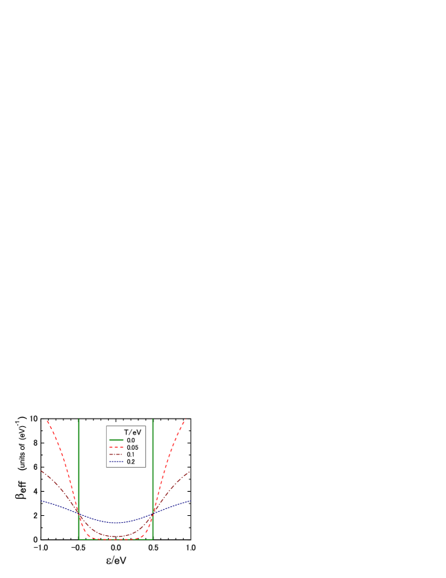
Figure 2: (color online). Parameter $\beta_{\mathrm{eff}}\equiv 1/\mathcal{T}_{\varepsilon}$, which determines the RDM as Eq. (36), is plotted as a function of $\varepsilon$ for several temperatures $T/(eV)=0.0,\,0.05,\,0.1$ and $0.2$, in the symmetric coupling case $\Gamma_{L}=\Gamma_{R}$.

Then, the average of an operator $\widehat{\cal O}_{S}=\widehat{\cal O}_{S}(\alpha,\alpha^{\dagger})$, which is an arbitrary function of $\alpha^{\phantom{\dagger}}_{\varepsilon,\sigma}$ and $\alpha^{\dagger}_{\varepsilon,\sigma}$, can be calculated in the $s$-wave subspace using the RDM,

$$\langle\widehat{\cal O}_{S}\rangle_{0}\equiv\mbox{Tr}_{S}^{\phantom{|}}\mbox{Tr}_{P}^{\phantom{|}}\!\left[\widehat{\rho}_{0}^{\phantom{S}}\widehat{\cal O}_{S}\right]=\mbox{Tr}_{S}^{\phantom{|}}\!\left[\widehat{\rho}_{0}^{S}\,\widehat{\cal O}_{S}\right].$$ (38)

Note that the impurity level has been included in the $s$-wave part. It is straight forward to confirm that $\langle\alpha^{\dagger}_{\varepsilon,\sigma}\alpha^{\phantom{\dagger}}_{\varepsilon^{\prime},\sigma^{\prime}}\rangle_{0}$ given in Eq. (15) can be reproduced from Eq. (38), and then the function $f_{\mathrm{eff}}(\varepsilon)$ defined in Eq. (16) can be expressed in terms of $\mathcal{T}_{\varepsilon}$ as

$$f_{\mathrm{eff}}(\varepsilon)=\frac{1}{e^{\varepsilon/\mathcal{T}_{\varepsilon}}+1}\;.$$ (39)

The bias dependence appears in the $s$-wave subspace through this energy-dependent parameter $\mathcal{T}_{\varepsilon}$. The inverse of this parameter, $\beta_{\mathrm{eff}}\equiv 1/\mathcal{T}_{\varepsilon}$, is plotted in Fig. 2 as a function of $\varepsilon$ for several values of real temperature $T$ in the symmetric coupling $\Gamma_{L}=\Gamma_{R}$ case. The energy dependence of $\mathcal{T}_{\varepsilon}$ becomes weak with increasing $T$. At zero temperature, it takes the form,

$$\mathcal{T}_{\varepsilon}\to\left\{\!\begin{array}[]{cl}\infty,&\ \ |\varepsilon|<eV/2,\\ 0,&\ \ |\varepsilon|>eV/2.\end{array}\right.$$ (42)

Namely, $\mathcal{T}_{\varepsilon}$ reaches infinity inside the energy window $|\varepsilon|<eV/2$, while it remain zero on the outside. For this reason, in the limit of $eV\to\infty$ the nonequilibrium Green’s functions at the impurity site coincide with the equilibrium ones for the high-temperature limit $T\to\infty$.OguriB

The partial trace over the $p$-wave part can be carried out also for $H_{U}\neq 0$, as the Coulomb interaction affects only the $s$-wave part of the Hilbert space. Therefore, the interacting RDM $\widehat{\rho}_{\phantom{0}}^{S}$ evolves adiabatically from the noninteracting RDM $\widehat{\rho}_{0}^{S}$ as

$$\widehat{\rho}_{\phantom{0}}^{S}= \,S(0,-\infty)\,\widehat{\rho}_{0}^{S}S(-\infty,0)\;,$$ (43)

$$\langle\widehat{\cal O}_{S}\rangle\equiv \,\mbox{Tr}_{S}^{\phantom{|}}\mbox{Tr}_{P}^{\phantom{|}}\!\left[\,\widehat{\rho}\ \widehat{\cal O}_{S}\right]=\mbox{Tr}_{S}^{\phantom{|}}\!\left[\,\widehat{\rho}_{\phantom{0}}^{S}\,\widehat{\cal O}_{S}\right]\;.$$ (44)

It enables us to treat the bias voltage within the $s$-wave part of the Hilbert space. Namely, one can start with the single-channel Anderson model $H^{S}$ in the continuous form, Eq. (20). Then, the nonequilibrium distribution can be taken into account through the initial RDM $\widehat{\rho}_{0}^{S}$, which evolves to the interacting one $\widehat{\rho}_{\phantom{0}}^{S}$. For the single-channel model, it is not necessary to use the same discretization scheme that was introduced to obtain Eq. (34), because $\widehat{\rho}_{0}^{S}$ has a well-defined continuum form as Eq. (36). In addition to these points, the correlation functions containing a $p$-wave operator can also be calculated with the single-channel model as shown in Appendix A.

IV Mixed-state aspect for $\Gamma_{L}=\Gamma_{R}$

As we see in Fig. 2, effects of the bias voltage are pronounced significantly at zero temperature, especially when the system has an inversion symmetry $\Gamma_{L}=\Gamma_{R}$. We consider in the following the properties of the RDM in this particular case.

At zero temperature $T=0$ the noninteracting density matrix $\widehat{\rho}_{0}^{\phantom{0}}$ for the whole system can be constructed as a pure state $\left|\Phi_{\rm neq}\right\rangle$, in which the scattering states incident from left and right are filled up to $\mu_{L}=eV/2$ and $\mu_{R}=-eV/2$, respectively,

$$\left|\Phi_{\rm neq}\right\rangle=\prod_{\varepsilon=0}^{\frac{eV}{2}}\prod_{\varepsilon^{\prime}=-\frac{eV}{2}}^{0}\prod_{\sigma}\widetilde{\gamma}_{\varepsilon,L\sigma}^{\dagger}\widetilde{\gamma}_{\varepsilon^{\prime},R\sigma}^{\phantom{\dagger}}\left|\Phi_{0}\right\rangle\;,$$ (45)

$$\left|\Phi_{0}\right\rangle\equiv\prod_{\varepsilon<0}\prod_{\sigma}\widetilde{\gamma}_{\varepsilon,L\sigma}^{\dagger}\widetilde{\gamma}_{\varepsilon,R\sigma}^{\dagger}\left|0\right\rangle=\prod_{\varepsilon<0}\prod_{\sigma}\widetilde{\alpha}_{\varepsilon\sigma}^{\dagger}\widetilde{p}_{\varepsilon\sigma}^{\dagger}\left|0\right\rangle.$$ (46)

Here, $\left|0\right\rangle$ is the vacuum state. The noninteracting ground state $\left|\Phi_{0}\right\rangle$ can be decomposed into the Fermi sea of the $s$-wave part $\left|\Phi_{0}^{S}\right\rangle$ and that of the $p$-wave part $\left|\Phi_{0}^{P}\right\rangle$ as $\left|\Phi_{0}\right\rangle=\left|\Phi_{0}^{S}\right\rangle\left|\Phi_{0}^{P}\right\rangle$. Therefore, Eq. (45) can be rewritten, using Eq. (11) for $v_{L}=v_{R}$, as

$$\left|\Phi_{\rm neq}\right\rangle =\,\prod_{\varepsilon=0}^{\frac{eV}{2}}\prod_{\varepsilon^{\prime}=-\frac{eV}{2}}^{0}\prod_{\sigma}\frac{(\widetilde{\alpha}_{\varepsilon\sigma}^{\dagger}-\widetilde{p}_{\varepsilon\sigma}^{\dagger})}{\sqrt{2}}\frac{(\widetilde{\alpha}_{\varepsilon^{\prime}\sigma}^{\phantom{\dagger}}+\widetilde{p}_{\varepsilon^{\prime}\sigma}^{\phantom{\dagger}})}{\sqrt{2}}\,\left|\Phi_{0}\right\rangle$$

$$=\,\frac{1}{\sqrt{Z_{0}}}\,{\sum_{i\in\mathcal{W}}}^{\prime}\left|\Phi_{i}^{S}\right\rangle\left|\Phi_{i}^{P}\right\rangle\;.$$ (47)

Here, $\left|\Phi_{i}^{S}\right\rangle$ and $\left|\Phi_{i}^{P}\right\rangle$ are the excited states of the $s$-wave part and that of the $p$-wave part, respectively: the sign caused by exchanges of the fermion operators is absorbed into the global phase of each many-particle eigenstate in the definition. The primed sum for $i$ runs over a set $\mathcal{W}$, which consists of all the possible excited states that can be generated from $\left|\Phi_{0}\right\rangle$ by changing the occupation of the one-particle states inside the biased energy region $|\varepsilon|<eV/2$. The factor $Z_{0}$ corresponds to the dimension of $\mathcal{W}$.

The pure-state average of an arbitrary operator $\widehat{\cal O}_{S}=\widehat{\cal O}_{S}(\alpha,\alpha^{\dagger})$ that is defined in the $s$-wave space can be calculated, carrying out the summation over the $p$-wave part, as

$$\left\langle\Phi_{\rm neq}\right|\widehat{\cal O}_{S}\left|\Phi_{\rm neq}\right\rangle=\frac{1}{Z_{0}}\,{\sum_{ij\in\mathcal{W}}}^{\prime}\!\left\langle\Phi_{i}^{P}\right|\!\!\left\langle\Phi_{i}^{S}\right|\widehat{\cal O}_{S}\left|\Phi_{j}^{S}\right\rangle\!\!\left|\Phi_{j}^{P}\right\rangle$$

$$\qquad\quad\ \ =\frac{1}{Z_{0}}\,{\sum_{i\in\mathcal{W}}}^{\prime}\!\left\langle\Phi_{i}^{S}\right|\widehat{\cal O}_{S}\left|\Phi_{i}^{S}\right\rangle=\mbox{Tr}_{S}^{\phantom{|}}\!\left[\,\widehat{\rho}_{0}^{S}\,\widehat{\cal O}_{S}\right].$$ (48)

Therefore in this case, the noninteracting RDM takes a mixed-state form $\widehat{\rho}_{0}^{S}=\sum_{n}\!\left|\Phi_{n}^{S}\right\rangle w_{0,n}^{S}\!\left\langle\Phi_{n}^{S}\right|$ with

$$w_{0,n}^{S}=\left\{\!\begin{array}[]{cl}1/Z_{0},&\quad n\in\mathcal{W},\\ 0,&\quad n\notin\mathcal{W}.\end{array}\right.$$ (51)

The summation with respect to $n$, or $\mbox{Tr}_{S}^{\phantom{|}}[\cdots]$, run over the whole region of the $s$-wave subspace. The statistical weight $w_{0,n}^{S}$ takes just two values $0$ or $1/Z_{0}$. However, it is not a simple function of the many-particle energy eigenvalue $E_{0,n}^{S}$ of $\widetilde{H}_{0}^{S}\left|\Phi_{n}^{S}\right\rangle=E_{0,n}^{S}\left|\Phi_{n}^{S}\right\rangle$.

There is another important relation between $\left|\Phi_{i}^{S}\right\rangle$ and $\left|\Phi_{i}^{P}\right\rangle$, as these states are generated simultaneously in Eq. (47). If a one-particle level $\varepsilon$ in the biased energy region $|\varepsilon|<eV/2$ is being occupied by an $s$-wave electron $\widetilde{\alpha}_{\varepsilon\sigma}^{\dagger}$ in $\left|\Phi_{i}^{S}\right\rangle$, then the corresponding level has to be unoccupied in the $p$-wave part $\left|\Phi_{i}^{P}\right\rangle$, or vice versa. Therefore, there exists a pair of states, $i$ and $i^{\prime}$, that show a relation $\widetilde{\alpha}_{\varepsilon\sigma}^{\phantom{\dagger}}\left|\Phi_{i}^{S}\right\rangle\!\left|\Phi_{i}^{P}\right\rangle=-\,\widetilde{p}_{\varepsilon\sigma}^{\phantom{\dagger}}\left|\Phi_{i^{\prime}}^{S}\right\rangle\!\left|\Phi_{i^{\prime}}^{P}\right\rangle$ for $|\varepsilon|<eV/2$. Here, the minus sign is caused by the order of the operators for the one-particle level $\varepsilon$. Using this property, a $p$-wave operator appearing in an average can be replaced by an $s$-wave operator as

$$\!\!\!\!\!\!\left\langle\Phi_{\rm neq}\right|\widehat{\cal O}_{S}\,p_{\varepsilon\sigma}\!\left|\Phi_{\rm neq}\right\rangle=\frac{1}{Z_{0}}{\sum_{ij\in\mathcal{W}}}^{\prime}\!\left\langle\Phi_{i}^{P}\right|\!\!\left\langle\Phi_{i}^{S}\right|\widehat{\cal O}_{S}\,p_{\varepsilon\sigma}\!\left|\Phi_{j}^{S}\right\rangle\!\!\left|\Phi_{j}^{P}\right\rangle$$

$$\qquad\qquad\quad=-\,\left[f_{L}(\varepsilon)-f_{R}(\varepsilon)\right]\,\mbox{Tr}_{S}^{\phantom{|}}\!\left[\widehat{\rho}_{0}^{S}\,\widehat{\cal O}_{S}\,\alpha_{\varepsilon\sigma}\right].$$ (52)

Similar relation holds also for the asymmetric coupling $\Gamma_{L}\neq\Gamma_{R}$ and at finite temperatures as shown in Appendix A.

The interacting density matrix at $T=0$ is also constructed as a pure state with the wavefunction

$$\left|\Psi_{\rm neq}\right\rangle\equiv S(0,-\infty)\left|\Phi_{\rm neq}\right\rangle=\frac{1}{\sqrt{Z_{0}}}{\sum_{i\in\mathcal{W}}}^{\prime}\left|\Psi_{i}^{S}\right\rangle\left|\Phi_{i}^{P}\right\rangle\;.$$ (53)

Here, $\left|\Psi_{n}^{S}\right\rangle\equiv S(0,-\infty)\left|\Phi_{n}^{S}\right\rangle$, and it is an interacting eigenstate,GML $(\widetilde{H}_{0}^{S}+H_{U})\left|\Psi_{n}^{S}\right\rangle=E_{n}^{S}\left|\Psi_{n}^{S}\right\rangle$. The wave function for the $p$-wave part keeps the noninteracting form, because $S(0,-\infty)$ commutes with the $p$-wave operators. Therefore, the summation over the $p$-wave part can be carried out in the same way as that in Eq. (48), and the interacting average for the operator $\widehat{\cal O}_{S}$ can be written in the form,

$$\left\langle\Psi_{\rm neq}\right|\widehat{\cal O}_{S}\left|\Psi_{\rm neq}\right\rangle =\frac{1}{Z_{0}}{\sum_{i\in\mathcal{W}}}^{\prime}\left\langle\Psi_{i}^{S}\right|\widehat{\cal O}_{S}\left|\Psi_{i}^{S}\right\rangle$$

$$=\sum_{n}w_{0,n}^{S}\!\left\langle\Psi_{n}^{S}\right|\widehat{\cal O}_{S}\left|\Psi_{n}^{S}\right\rangle.$$ (54)

The interacting RDM in this case also takes a simple form $\widehat{\rho}_{\phantom{0}}^{S}=\sum_{n}\left|\Psi_{n}^{S}\right\rangle w_{0,n}^{S}\!\left\langle\Psi_{n}^{S}\right|$. Equation (54) gives us much insight into the steady state. It will provide, obviously, an interacting equilibrium average if we replace $w_{0,n}^{S}$ by $\rho_{\mathrm{eq},n}^{S}\equiv e^{-\beta E_{n}^{S}}\!/\!\sum_{n}\!e^{-\beta E_{n}^{S}}$. Therefore, some of the nonequilibrium properties could be inferred from the difference between the statistical weights $w_{0,n}^{S}$ and $\rho_{\mathrm{eq},n}^{S}$.

As Eq. (54) is being expressed in terms of the interacting eigenstates, Hamiltonian-based nonperturbative approaches developed for equilibrium, such as exact diagonalization and NRG, can be applied to the matrix element $\left\langle\Psi_{n}^{S}\right|\!\widehat{\cal O}_{S}\!\left|\Psi_{n}^{S}\right\rangle$. Furthermore, the bias voltage appears just through $w_{0,n}^{S}$, which keeps the noninteracting form given in Eq. (51). Thus, what is necessary to carry out the summation with respect to $n$ in Eq. (54) is the information about whether or not each interacting eigenstate $\left|\Psi_{n}^{S}\right\rangle$ belongs to the set $\mathcal{W}$ in the limit of $H_{U}\to 0$. Namely, the correspondence between $\left|\Psi_{i}^{S}\right\rangle$ and its noninteracting counterpart $\left|\Phi_{i}^{S}\right\rangle$ is an additional issue that one has to solve in the nonequilibrium case. At low energies, the correspondence can be treated correctly with the quasi-particles of a local Fermi liquid.Hewson ; KNG ; OguriA ; FujiiUeda ; GogolinKomnik ; HB

The evolution of the wavefunctions is described formally with the time-dependent operator $S(0,-\infty)$. Alternatively, it can be expressed in a time-independent form as that in a stationary-state scattering theory,GML ; GMGB and several versions of the time-independent approaches have been examined with some different points of view. SchillerHershfield ; KSL ; KNG ; Han ; MehtaAndrei In our description, the adiabatic evolution of the interacting eigenstates from the noninteracting ones could also be traced directly in the Hilbert space of a discretized version of the single-channel model, by changing the coupling constant $U$ continuously.

V Energy distribution in the mixed states

We consider in the following the mixed-sate properties for the symmetric coupling $\Gamma_{L}=\Gamma_{R}$ further at $T=0$. The pure state $\left|\Phi_{\rm neq}\right\rangle$ given in Eq. (45) is an eigenstate, $\widetilde{H}_{0}\left|\Phi_{\rm neq}\right\rangle=E_{0}^{\mathrm{neq}}\left|\Phi_{\rm neq}\right\rangle$, of the noninteracting Hamiltonian with an excitation energy

$$E_{0}^{\mathrm{neq}}\,=\,2\!\sum_{\varepsilon_{m}=-eV/2}^{eV/2}|\varepsilon_{m}|\xrightarrow[\ \delta\varepsilon\to 0\ ]{}\frac{\left(eV\right)^{2}}{2\,\delta\varepsilon}\;.$$ (55)

Here, we retained only the dominant term that is proportional to the system size of order $N$. As mentioned in Sec. III, the level spacing is given by $\delta\varepsilon=2D/N$ for a flat band with a half width $D$. The feature of the pure state reflects in the $s$-wave subspace through the RDM. The mean excitation energy in the subspace is equal to a half of the one in Eq. (55), $\overline{E}_{0}^{S}\equiv\mbox{Tr}_{S}^{\phantom{|}}\bigl{[}\widehat{\rho}_{0}^{S}\widetilde{H}_{0}^{S}\bigr{]}=E_{0}^{\mathrm{neq}}/2$. Note that the contribution of the impurity level is of order $1$, namely a $1/N$ portion of the total energy.

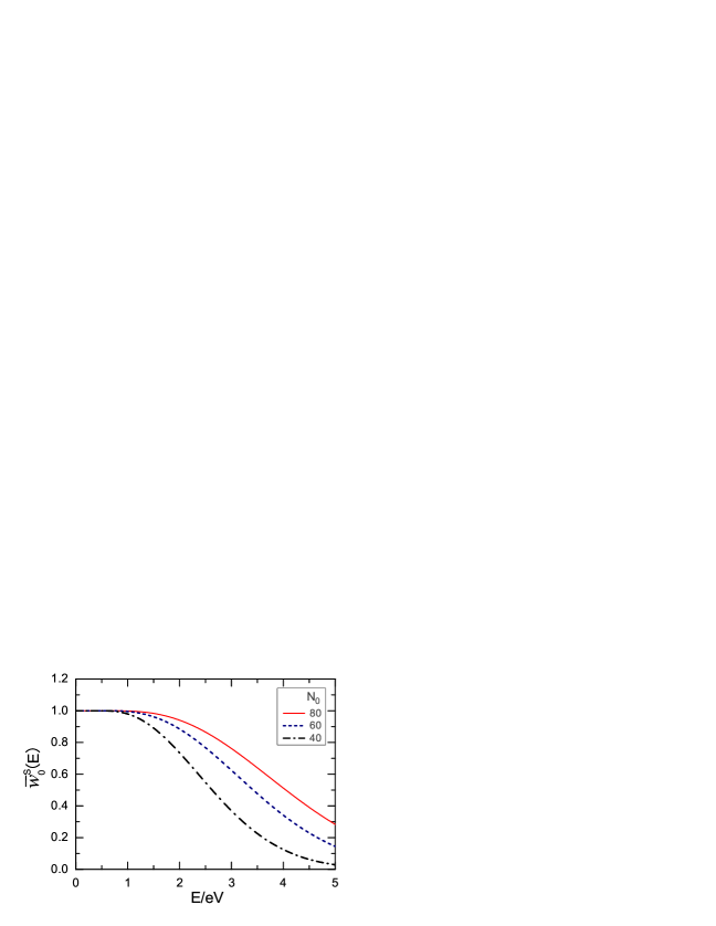
Figure 3: (color online). Averaged statistical weight $\overline{w}_{0}^{S}(E)\equiv W(E)\,/\,\Omega(E)$ vs many-particle excitation energy $E$, where $N_{0}=eV/\delta\varepsilon$.

In order to clarify how the nonequilibrium weight $w_{0,n}^{S}$ distributes in the many-particle Hilbert space consisting of the eigenstates $\left|\Phi_{n}^{S}\right\rangle$, we examine an averaged weight $\overline{w}_{0}^{S}(E)$ over an equienergy surface;

$$\overline{w}_{0}^{S}(E)\,\equiv\,W(E)\,/\,\Omega(E)\;,$$ (56)

$$\!\!\!W(E)=\!{\sum_{i\in\mathcal{W}}}^{\prime}\!\delta(E-E_{0,i}^{S}),\ \ \Omega(E)=\!\sum_{n}\delta(E-E_{0,n}^{S}).$$ (57)

It is normalized as $Z_{0}=\int\!dE\ \overline{w}_{0}^{S}(E)\Omega(E)$, and may be used as $\left\langle\Psi_{\rm neq}\right|\!\widehat{\cal O}_{S}\!\left|\Psi_{\rm neq}\right\rangle\approx\!\sum_{n}\overline{w}_{0}^{S}(E_{n}^{S})\left\langle\Psi_{n}^{S}\right|\!\widehat{\cal O}_{S}\!\left|\Psi_{n}^{S}\right\rangle\!/Z_{0}$ for a rough approximation. We calculate $\overline{w}_{0}^{S}(E)$ for several finite $\delta\varepsilon$, and the results are shown in Fig. 3: the parameter $N_{0}\equiv eV/\delta\varepsilon$ corresponds to the number of one-particle states in the energy window $|\varepsilon|<eV/2$, and thus $Z_{0}=4^{N_{0}}$. The averaged weight $\overline{w}_{0}^{S}(E)$ becomes a constant for small $E$, as all the many-particle excited states for $0<E<eV/2$ belong to the set $\mathcal{W}$ defined in Eq. (47). This flat $E$-dependence is quite different from the exponential dependence of the Boltzmann factor $e^{-\beta E}$ in the thermal equilibrium. We also see that $\overline{w}_{0}^{S}(E)$ penetrates into the higher energy region over the bias energy $eV$. It spreads out, approximately, up to $E\sim c\,\overline{E}_{0}^{S}$ with a numerical constant $c$ of order $10^{-1}$. Note that the mean excitation energy is proportional to $N_{0}$ as $\overline{E}_{0}^{S}=N_{0}eV/4$. We have also obtained the analytic expressions of $\Omega(E)$ and $W(E)$ for small $\delta\varepsilon$ as shown in Appendix B, and have checked that the same behavior could be seen for larger $N_{0}$ assuming a Gaussian form for $W(E)$ given in Eq. (66), instead of the exact integration form Eq. (65).

The feature of $\overline{w}_{0}^{S}(E)$ seen in the $s$-wave subspace is caused by the fact that the bias voltage has been introduced not into the many-particle energy but into the one-particle states as the width of the energy window between the two chemical potentials $\mu_{L}$ and $\mu_{R}$. It is quite different from the way the temperature determines the equilibrium distribution $e^{-E/T}$, in which $T$ scales directly the many-particle energy $E$. The original weight $w_{0,n}^{S}$ must have the similar features in the $n$ dependence. However, whether or not the high-energy many-particle states give significant contributions to the nonequilibrium averages depends also on the properties of the operator $\widehat{\cal O}_{S}$. For instance, the noninteracting correlation functions, such as $\langle\alpha^{\dagger}_{\varepsilon,\sigma}\alpha^{\phantom{\dagger}}_{\varepsilon^{\prime},\sigma^{\prime}}\rangle_{0}$ and $G^{<}_{0}(\varepsilon)$, can be reproduced from Eq. (48). The feature of $w_{0,n}^{S}$ reflects in these correlation functions just through $f_{\mathrm{eff}}(\varepsilon)$. It should be regarded, however, those are the results that are determined by all the many-particle states belonging to the set $\mathcal{W}$. Therefore, it is necessary for calculating the interacting Green’s functions with Eq. (54) to take all these high-energy states into account. The Kondo resonance at finite bias voltages is being affected by these features of the nonequilibrium distribution.

VI Summary

In conclusion, we have reexamined the nonequilibrium steady state for a quantum dot, checking out the statistical distribution in the many-particle Hilbert space. We have, first of all, discretized the conduction bands keeping the two-fold degeneracy due to the left-going and right-going scattering states. This degeneracy is essential to describe the current-carrying state driven by the bias voltage. Then, by integrating out the $p$-wave part of the channel degrees of freedom, the noninteracting RDM $\widehat{\rho}_{0}^{S}$ has been obtained explicitly as shown in Eq. (35). It brings the information about the bias voltages to the remaining $s$-wave subspace, and determines the nonequilibrium distribution. The interacting RDM $\widehat{\rho}^{S}$, which is defined in Eq. (43), evolves adiabatically from $\widehat{\rho}_{0}^{S}$. Using the RDM, the steady-state averages Eq. (44) can be calculated, in principle, with the single-channel Anderson model.

We have studied further the properties of the RDM at zero temperature for the symmetric coupling $\Gamma_{L}=\Gamma_{R}$. In this case the nonequilibrium averages can be written in a Lehmann-representation form Eq. (54) with a simple mixed-state distribution $w_{0,n}^{S}$ given in Eq. (51). It has also been deduced that the mixed states contain large portions of high-energy many-particle states. Our formulation could be used for constructing Hamiltonian-based nonperturbative approaches in future.

Appendix A RDM approach to the $p$-wave operator

The correlation functions which include a $p$-wave operator can be expressed, using Eq. (33), as

$$\langle\widehat{\cal O}_{S}\,p^{\phantom{\dagger}}_{\varepsilon\sigma}\rangle_{0}=\lim_{\delta\varepsilon\to 0}\mbox{Tr}_{S}^{\phantom{|}}\mbox{Tr}_{P}^{\phantom{|}}\!\left[\,\widetilde{\rho}_{0}\,\widehat{\cal O}_{S}\,\widetilde{p}^{\phantom{\dagger}}_{\varepsilon,\sigma}\right]/\,\sqrt{\delta\varepsilon}$$

$$\qquad=-\frac{v_{L}^{\phantom{|}}v_{R}^{\phantom{|}}}{v_{R}^{2}+v_{L}^{2}}\frac{f_{L}(\varepsilon)-f_{R}(\varepsilon)}{f_{\mathrm{eff}}(\varepsilon)}\,\mbox{Tr}_{S}^{\phantom{|}}\!\left[\widehat{\rho}_{0}^{S}\,\widehat{\cal O}_{S}\,\alpha^{\phantom{\dagger}}_{\varepsilon\sigma}\right]$$ (58)

in the noninteracting case. For instance, Eq. (17) can be reproduced from Eq. (58) for $\widehat{\cal O}_{S}=\alpha_{\varepsilon^{\prime}\sigma^{\prime}}^{\dagger}$. The interacting average can also be expressed in a similar form

$$\langle\widehat{\cal O}_{S}\,p^{\phantom{\dagger}}_{\varepsilon\sigma}\rangle=-\frac{v_{L}^{\phantom{|}}v_{R}^{\phantom{|}}}{v_{R}^{2}+v_{L}^{2}}\frac{f_{L}(\varepsilon)-f_{R}(\varepsilon)}{f_{\mathrm{eff}}(\varepsilon)}\,$$

$$\qquad\qquad\times\mbox{Tr}_{S}\left[\widehat{\rho}_{0}^{S}\,S(-\infty,0)\,\widehat{\cal O}_{S}\,S(0,-\infty)\,\alpha_{\varepsilon\sigma}^{\phantom{\dagger}}\right].$$ (59)

Appendix B $\Omega(E)$ and $W(E)$ for small $\delta\varepsilon$

We provide the integration forms of $\Omega(E)$ and $W(E)$ for small level spacing $\delta\varepsilon$. To this end, we consider a grand partition function $\mathcal{G}(\tau,E_{c})$ for noninteracting electrons in a flat band with the cut-off $E_{c}$. The grand partition function and many-particle density of states $F(E,E_{c})$ are relating each other with the Laplace transform,

$$\mathcal{G}(\tau,E_{c})=\int_{0}^{\infty}\!\!dE\ e^{-\tau E}\,F(E,E_{c})\;.$$ (60)

For small $\delta\varepsilon$, the left-hand side, $\mathcal{G}(\tau,E_{c})$, is given by

$$\prod_{\sigma}\prod_{\lambda=e,h}\prod_{\varepsilon=0}^{E_{c}}\left(1+e^{-\varepsilon\tau}\right)\Rightarrow\prod_{\sigma}\frac{1+e^{-\tau E_{c}}}{2}\ e^{\frac{\scriptstyle 2}{\scriptstyle\delta\varepsilon}\,X(\tau,E_{c})},$$ (61)

$$\!\!\!X(\tau,E_{c})\equiv\!\!\int_{0}^{E_{c}}\!\!\!d\varepsilon\,\ln\left(1+e^{-\varepsilon\tau}\right)=\frac{\phi(0)-\phi(\tau E_{c})}{\tau}.$$ (62)

Here, $\phi(z)=\sum_{m=1}^{\infty}\frac{(-1)^{m-1}}{m^{2}}e^{-mz}$ and $\phi(0)=\pi^{2}/12$. The label $\lambda$ represents the contributions of the electron ($e$) and hole ($h$) excitations. The function $F(E,E_{c})$ is given as the inverse Laplace transform

$$F(E,E_{c})=\!\!\int_{\tau_{0}-i\infty}^{\tau_{0}+i\infty}\!\!\frac{d\tau}{2\pi i}\,e^{\tau E}\,\frac{\left(1+e^{-\tau E_{c}}\right)^{2}}{4}e^{\frac{\scriptstyle 4}{\scriptstyle\delta\varepsilon}\frac{\scriptstyle\phi(0)-\phi(\tau E_{c})}{\scriptstyle\tau}}.$$ (63)

The function $\Omega(E)=F(E,\infty)$ is obtained taking the limit of $E_{c}\to\infty$: then $e^{-\tau E_{c}}\to 0$, $\phi(\tau E_{c})\to 0$, and the integration can be carried out for $E>0$,

$$\Omega(E)\, =\,\frac{1}{4}\sqrt{\frac{4\phi(0)}{E\,\delta\varepsilon}}\ I_{1}\!\left(2\sqrt{{4\phi(0)E}/{\delta\varepsilon}}\right)\>.$$ (64)

Here, $I_{1}(x)$ is the modified Bessel function, which for large $x$ takes the asymptotic form; $I_{1}(x)\simeq e^{x}/\sqrt{2\pi x}$.

The other function $W(E)=F(E,eV/2)$ is obtained for $E_{c}=eV/2$. Note that $W(E)=\Omega(E)$ for $0<E<E_{c}$ because the cut-off does not affects the excitations in this energy region. Furthermore, $W(E)=0$ for $E>2E_{c}(N_{c}+1)$ beyond an upper bound, where $N_{c}=E_{c}/\delta\varepsilon$. Equation (63) can be rewritten taking the path along the imaginary axis as

$$\!W(E)=\!\int_{-\infty}^{\infty}\!\!\frac{dt}{2\pi}\,e^{iEt}\frac{\left(1+e^{-itE_{c}}\right)^{2}}{4}e^{\frac{\scriptstyle 4}{\scriptstyle\delta\varepsilon}\frac{\scriptstyle\phi(0)-\phi(itE_{c})}{\scriptstyle it}}.$$ (65)

Note that $\mbox{Re}\bigl{[}\phi(0)-\phi(ix)\bigr{]}=x^{2}/4$ for $-\pi<x<\pi$. Thus, $W(E)$ has a peak at $E=E_{c}(N_{c}+1)$, and around the peak it may be approximated in a Gaussian form

$$\!\!W(E)\approx\frac{4^{2N_{c}}}{E_{c}}\sqrt{\frac{3}{\pi(2N_{c}+3)}}\ e^{-\frac{3}{(2N_{c}+3)}\left(\frac{E}{E_{c}}-N_{c}-1\right)^{2}}.$$ (66)

This approximate form overestimates $W(E)$ for small $E$, suggesting that the real density given by Eq. (65) has larger weight around the peak than that of the Gaussian.

References

- (1) L. I. Glazman and M. E. Raikh, JETP Lett. 47, 452 (1988).
- (2) T. K. Ng and P. A. Lee, Phys. Rev. Lett. 61, 1768 (1988).
- (3) D. Goldharber-Gordon, H. Shtrikman, D. Mahalu, D. Abusch-Magder, U. Meirav, and M. A. Kastner, Nature 391, 156 (1998).
- (4) S. M. Cronenwett, T. H. Oosterkamp, and L. P. Kouwenhoven, Science 281, 540 (1998).
- (5) F. Simmel, R. H. Blick, J. P. Kotthaus, W. Wegscheider, and M. Bichler, Phys. Rev. Lett. 83, 804 (1999).
- (6) W. G. van der Wiel, S. De Franceschi, T. Fujisawa, J. Elzerman, S. Tarucha, and L. P. Kouwenhoven, Science 289, 2105 (2000).
- (7) A. C. Hewson, The Kondo Problem to Heavy Fermions (Cambridge University Press, Cambridge, 1993).
- (8) N. S. Wingreen and Y. Meir, Phys. Rev. B 49, 11040 (1994).
- (9) S. Hershfield, J. H. Davies, and J. W. Wilkins, Phys. Rev. B 46, 7046 (1992).
- (10) A. L. Yeyati, A. Martin-Rodero, and F. Flores, Phys. Rev. Lett. 71, 2991 (1993); M. H. Hettler, J. Kroha, and S. Hershfield, Phys. Rev. Lett. 73, 1967 (1994); H. Schoeller and J. König, Phys. Rev. Lett. 84, 3686 (2000); A. Rosch, J. Kroha and P. Wölfle, Phys. Rev. Lett. 87, 156802 (2001); P. Coleman, C. Hooley, and O. Parcollet, Phys. Rev. Lett. 86, 4088 (2001); O. Parcollet and C. Hooley, Phys. Rev. B 66, 085315 (2002).
- (11) R. M. Konik, H. Saleur, and A. Ludwig, Phys. Rev. B 66, 125304 (2002).
- (12) A. Schiller and S. Hershfield, Phys. Rev. B 58, 14978 (1998).
- (13) A. Kaminski, Yu. V. Nazarov, and L. I. Glazman, Phys. Rev. B 62, 8154 (2000).
- (14) A. Oguri, Phys. Rev. B 64, 153305 (2001); J. Phys. Soc. Jpn. 74, 110 (2005).
- (15) A. Oguri, J. Phys. Soc. Jpn. 71, 2969 (2002).
- (16) T. Fujii and K. Ueda, Phys. Rev. B 68, 155310 (2003); J. Phys. Soc. Jpn. 74, 127 (2005).
- (17) A. O. Gogolin and A. Komnik, Phys. Rev. B 73, 195301 (2006); Phys. Rev. Lett. 97, 016602 (2006).
- (18) A. C. Hewson, J. Bauer, and A. Oguri, J. Phys.: Condes. Matter. 17, 5413 (2005).
- (19) L. V. Keldysh, Sov. Phys. JETP 20 1017 (1965).
- (20) C. Caroli, R. Combescot, P. Nozieres, and D. Saint-James, J. Phys. C 4, 916 (1971).
- (21) H. R. Krishna-murthy, J. W. Wilkins, and K. G. Wilson, Phys. Rev. B 21, 1003 (1980).
- (22) R. M. Fye and J. E. Hirsch, Phys. Rev. B 38, 433 (1988).
- (23) S. Hershfield, Phys. Rev. Lett. 70, 2134 (1993).
- (24) J. E. Han, Phys. Rev. B 73, 125319 (2006); cond-mat/0604583.
- (25) Y. Meir and N. S. Wingreen, Phys. Rev. Lett. 68, 2512 (1992).
- (26) M. Gell-Mann and F. Low, Phys. Rev. 84, 350 (1951).
- (27) M. Gell-Mann and M. L. Goldberger, Phys. Rev. 91, 398 (1953).
- (28) P. Mehta and N. Andrei, Phys. Rev. Lett. 96, 216802 (2006).