Switching speed distribution of spin-torque-induced magnetic reversal

Abstract

The switching probability of a single-domain ferromagnet under spin-current excitation is evaluated using the Fokker-Planck equation(FPE). In the case of uniaxial anisotropy, the FPE reduces to an ordinary differential equation in which the lowest eigenvalue $\lambda_{1}$ determines the slowest switching events. We have calculated $\lambda_{1}$ by using both analytical and numerical methods. It is found that the previous model based on thermally distributed initial magnetization states Sun1 can be accurately justified in some useful limiting conditions.

I Introduction

Fast and reliable nanosecond level writing is essential for spin-torque-induced switching in memory and recording technologies. One intrinsic source for write threshold distribution is thermal fluctuation, two aspects of which could affect reversal time $\tau_{s}$. First, the initial position of the magnetic moment is thermally distributed at the time the reversal field or current is applied, causing a variation in switching time. Secondly, during reversal, thermal fluctuation would modify the orbit, causing additional fluctuation for $\tau_{s}$ even for identical initial conditions. A reversal time distribution due to a thermalized initial condition was recently estimated Sun1 . Here we present a Fokker-Planck formulation for the full problem including both thermalized initial condition and reversal orbit with estimates for the reversal time and its distribution.

Fokker-Planck equations have been successfully applied to macro-spin systems with a static thermal distribution for the extraction of a small thermal escape probability. For example, the distribution for a thermally activated reversal has been analytically and numerically obtained when the applied magnetic field is smaller than the coercive field Brown ; Aharoni ; Scully ; Coffey ; Bertram . There the switching is through thermally assisted transition from one metastable energy minimum to equilibrium. The ensemble-averaged $\tau_{s}$ depends exponentially on the ratio between the reversal energy barrier and thermal energy $k_{B}T$. These subthreshold results have recently been extended to include the effect of spin-torque, which modifies the effective temperature Zhang ; Visscher ; Sun2 .

For fast, dynamically driven switching, the applied spin-torque is above the zero-temperature reversal threshold. For finite temperature, this leads to a time-dependent Fokker-Planck equation in which the time-evolution of the probability represents the thermalized reversal of the macro-spin. Here we solve this problem in the colinear geometry with a uniaxial anisotropy energy landscape and the presence of a spin torque.

II Fokker-Planck equation

Consider an ensemble time-dependent magnetization probability density $P({\bf{n}_{m}},t)$, where $\bf{n}_{m}$ is the unit vector describing the direction of the macro-spin moment $\bf m$; in spherical coordinates ${\bf n_{m}}$ is characterized by $(\theta,\phi)$. Before one turns on the magnetic field and the current, the probability density takes its equilibrium value. For a uniaxial anisotropy-only situation,

$$P({\bf{n}_{m}},0)=P_{0}\exp(-\xi\sin^{2}\theta)$$ (1)

for $0\leq\theta\leq\pi/2$ and $P({\bf{n}_{m}},0)=0$ for $\pi/2<\theta\leq\pi$, where $P_{0}$ is the normalization factor ($\int_{0}^{\pi}P\sin\theta d\theta=1$), $P_{0}\approx 2\xi$, if we consider $\xi\equiv KV/k_{B}T\gg 1$ where $K$ is the anisotropy constant and $V$ is the volume of nanomagnet. To determine $P({\bf{n}_{m}},t)$ after one turns on the field and the current at $t=0$, we need to solve the Fokker-Planck equation given below

$$\frac{\partial P}{\partial t}+\nabla\cdot{\bf J}-D\nabla^{2}P=0$$ (2)

where ${\bf J}$ is the probability current and $D=\alpha\gamma k_{B}T/m$ is the diffusion constant, $\alpha$ is the damping parameter, $\gamma$ is the gyromagnetic coefficient, and $m=|\bf m|$. The probability current is

$${\bf J}=P\frac{d{\bf{n}_{m}}}{dt}=-\gamma P{\bf{n}_{m}}\times[{\bf H}_{e}+\alpha{\bf{n}_{m}}\times({\bf H}_{e}-{\bf H}_{s})]$$ (3)

where we have used the Landau-Lifshitz-Gilbert equation including the spin torque term ${\bf H}_{s}=(Ip)(\hbar/2q)(1/\alpha m){\bf n}_{s}$ ($I$ is current density, $p$ is the spin polarization coefficient, $q$ is the electron charge, and ${\bf n}_{s}$ is a unit vector in the direction of the magnetization of the pinned layer). To make the solution mathematically tractable, we consider the case where the magnetic field ${\bf H}$ and ${\bf n}_{s}$ are parallel to the anisotropy axis, i.e., ${\bf H}_{e}=(H+H_{k}\cos\theta){\bf e}_{z}$ and ${\bf n}_{s}={\bf e}_{z}$ where $H_{k}=2K/M_{s}$. With these simplifications, Eq. (3) reduces to

$$\frac{\partial P}{\partial t}=\frac{\alpha\gamma}{m}\frac{\partial}{\partial x}\left[(1-x^{2})\left(\frac{\partial U_{e}}{\partial x}P+k_{B}T\frac{\partial P}{\partial x}\right)\right]$$ (4)

where $x=\cos\theta$, and we have defined the effective potential $U_{e}=(H_{s}-H)mx-(H_{k}/2)mx^{2}$. Equation (4) can be solved via the method of separation of variables. Let’s assume $P(x,t)=f(t)u(x)$ and it is easy to see that $f(t)=\exp(-\lambda t)$ and $u(x)$ satisfies

$$\frac{\alpha\gamma}{m}\frac{d}{dx}\left[(1-x^{2})\left(\frac{dU_{e}}{dx}u(x)+k_{B}T\frac{du(x)}{dx}\right)\right]=-\lambda u(x)$$ (5)

The above equation can be converted into a Sturm-Liouville equation,

$$\frac{d}{dx}\left[(1-x^{2}){\rm e}^{-\beta U_{e}}\frac{dF}{dx}\right]+{c}{\rm e}^{-\beta U_{e}}F=0$$ (6)

where $F(x)={\rm e}^{\beta U_{e}(x)}u(x)$ and $c=\lambda m/\alpha\gamma k_{B}T$. Equation (6) is the same equation introduced by Brown Brown except that $U_{e}$ includes the spin-current term $H_{s}$. The original FPE (4) is now reduced to the standard eigenvalve problem. Namely, we determine eigen-function $F(x)=F_{n}(x)$ and eigenvalue $\lambda=\lambda_{n}$ from Eq. (6) for $n=0,1,2,...$, and the general solution of Eq. (4) is

$$P(x,t)=\sum_{n=0}A_{n}e^{-\beta U_{e}(x)}F_{n}(x){\rm e}^{-\lambda_{n}t}$$ (7)

where the coefficients in Eq. (7) are determined by the initial condition Eq. (1): $A_{n}=\int_{-1}^{1}dxP(x,0)F_{n}(x)$, where we have chosen the eigenfunction $F_{n}(x)$ to be weighted normalized: $\int_{-1}^{1}dx{\rm e}^{-\beta U_{e}(x)}F^{2}_{n}(x)=1$.

The remaining task is to solve eigenvalue $\lambda_{n}$ (or $c_{n}$) and eigenfunction $F_{n}$. Obviously, $\lambda_{0}=0$ is the lowest eigenvalue with the corresponding eigenfunction $F_{0}$ being a constant. Thus, $u_{0}(x)\propto\exp(-\beta U_{e})$ describes the thermal equilibrium state. The smallest nonzero eigenvalue $\lambda_{1}$ then determines the slowest decaying or switching speed.

The early theoretical attempts toward solving Eq. (6) Brown ; Aharoni ; Coffey ; Scully ; Bertram had been focused on the cases where there are two potential wells separated by an energy barrier and $H<H_{k}$. These solutions do not apply to the fast switching case where $H>H_{k}$. In this case, there is no energy barrier and the only stable solution is at $x=-1$ or $\theta=\pi$. In the following, we develop two methods to solve the Eq. (6): one is the approximate minimization which provides an upper bound for $\lambda_{1}$ and the other is to numerically determine the coefficients of polynomial series when Eq. (6) is expanded into polynomials.

The variational method can be obtained by multiplying $F(x)$ to Eq.(6) and then by integrating from -1 to 1,

$$\int_{-1}^{1}dxF\frac{d}{dx}\left[(1-x^{2}){\rm e}^{-\beta U_{e}}\frac{dF}{dx}\right]+c\int_{-1}^{1}{\rm e}^{-\beta U_{e}}F^{2}dx=0.$$

Performing integration by parts of the first term, we find

$$c={\cal D}/{\cal H}$$ (8)

where

$$\left\{\begin{array}[]{ll}{\cal D}=\int_{-1}^{1}dx{\rm e}^{-\beta U_{e}}(1-x^{2})\left(\frac{dF}{dx}\right)^{2}\\ \\ {\cal H}=\int_{-1}^{1}dx{\rm e}^{-\beta U_{e}}F^{2}(x)\end{array}\right.$$ (9)

Since both ${\cal D}$ and ${\cal H}$ are definitely positive, the variational principle is to choose a trial function $F(x)$ such that $c$ is minimized, and the non-zero minimum $c$ represents the upper bound of the lowest eigenvalue $c_{1}$. Additional constriction of $F(x)$ is its orthogonality with $F_{0}$ which is a constant, i.e.,

$$\int_{-1}^{1}{\rm e}^{-\beta U_{e}}F(x)dx=0.$$ (10)

Since $\exp(-\beta U_{e})$ is sharply peaked at $x=-1$ in our case, we change the variable as $x=y-1$ and thus $\beta U_{e}=\eta y-\xi y^{2}+const$, where we define $\eta=\frac{m}{k_{B}T}(H_{s}-H+H_{k})$ and $\xi=\frac{m}{k_{B}T}\frac{1}{2}H_{k}$. We consider a simple trial function $F(y)=1+b_{1}y+b_{2}y^{2}$ where $b_{1}$ and $b_{2}$ are variational parameters. By placing $F(y)$ into Eq. (9) and (10), we have

$$\left\{\begin{array}[]{ll}{\cal D}=\int_{0}^{2}y(2-y){\rm e}^{-\eta y+\xi y^{2}}(b_{1}+2b_{2}y)^{2}dy\\ \\ {\cal H}=\int_{0}^{2}{\rm e}^{-\eta y+\xi y^{2}}(1+b_{1}y+b_{2}y^{2})^{2}dy\\ \\ \int_{0}^{2}{\rm e}^{-\eta y+\xi y^{2}}(1+b_{1}y+b_{2}y^{2})dy=0\end{array}\right.$$ (11)

After the completion of these three integrations, the eigenvalue $c_{1}$ is obtained by minimizing $\cal D/H$ with respect to $b_{2}$ or $b_{1}$. The above integrations can be analytically obtained if we we notice that $y$ is limited to $1/\eta$ due to exponential ${\rm e}^{-\eta y}$ and thus the term $e^{\xi y^{2}}$ is small and can be expanded as: ${\rm e}^{\xi y^{2}}=1+\xi y^{2}+\frac{1}{2}\xi^{2}y^{4}$. By using $\int_{0}^{2}y^{n}{\rm e}^{-\eta y}dy\approx n!/\eta^{n+1}$, for example, the third equation in Eq. (11) is

$$\frac{1}{\eta}+\frac{2\xi}{\eta^{3}}+\frac{12\xi^{2}}{\eta^{5}}+\left(\frac{1}{\eta^{2}}+\frac{6\xi}{\eta^{4}}+\frac{60\xi^{2}}{\eta^{6}}\right)b_{1}$$

$$+\left(\frac{2}{\eta^{3}}+\frac{24\xi}{\eta^{5}}+\frac{360\xi^{2}}{\eta^{7}}\right)b_{2}=0$$ (12)

Note that the leading orders of $b_{1}$ and $b_{2}$ are $\eta$ and $\eta^{2}$ respectively, and the above equation is valid up to $\eta^{-3}$. If we consider the fast switching case, i.e. $\eta\gg\xi$, or $H_{s}-H\gg H_{k}$, the equation (12) can be further approximated as

$$b_{1}=-2b_{2}\eta^{-1}-\eta$$ (13)

We can similarly calculate $\cal H$ and $\cal D$. Substituting $b_{1}$ by Eq. (13), the expression of $\cal D/H$ contains only $b_{2}$. Then, we find $b_{2}$ by minimizing $\cal D/H$

$$\frac{d}{db_{2}}\left(\frac{\cal D}{\cal H}\right)=0$$ (14)

The results are:

$$\left\{\begin{array}[]{lll}b_{2}=\frac{1}{2}\eta^{2},&b_{1}=-2\eta&\\ \\ {\cal H}=\frac{1}{\eta},&{\cal D}=4,&c_{1}=\frac{\cal D}{\cal H}=4\eta\end{array}\right.$$

Rewriting in terms of original parameters, we find the slowest decaying rate is

$$\lambda_{1}=4\alpha\gamma\left(H_{s}-H\right)=4(I/I_{c}-1)\tau_{0}^{-1}$$ (15)

where $\tau_{0}^{-1}=\frac{p\mu_{B}}{qm}I_{c}=\alpha\gamma(H+H_{k})$.

Although the variational method is able to analytically obtain the upper bound for the rate of the relaxation, its accuracy is unknown. A more rigorous method is to expand $F(x)$ via Taylor series, i.e., $F(x)=\sum a_{n}x^{n}$ ($n=0,1,2...$). By substituting it into Eq. (6),we find the recurrence formula for coefficient $a_{n}$

$$(n+2)(n+1)a_{n+2}-\zeta(n+1)a_{n+1}$$

$$+[c_{n}-n(n-1)+n(2\xi-2)]a_{n}$$

$$+\zeta(n-1)a_{n-1}-2\xi(n-2)a_{n-2}=0$$ (16)

where $\zeta=\eta-2\xi=\frac{m}{k_{B}T}(H_{s}-H)$. In the case of $\zeta=\xi=0$, the above equation reduces to a two-term recursion formula, and the solutions are the Legendre polynomials with $c_{n}=n(n+1)$. This is the well-known solution for the thermal decay of a free particle Brown . In the case of $\zeta=0$, Eq. (16) reduces to a three-term recursion formula, and the continued fraction method can be used to obtain the smallest nonzero eigenvalue $c_{1}=2-\frac{4}{5}\xi+O(\xi^{2})$Aharoni .

In our case where both $\zeta$ and $\xi$ are non-zero, above methods can not be used directly. One way to solve the problem is to numerically calculate Eq. (16) by simply keeping enough terms (i.e. up to a large number $N=300$) to ensure the convergence of $c_{1}$. In Fig. 1,we show that the relaxation rates as a function of temperature ($H_{k}$ is fixed) for different $I/I_{c}(\geq 1)$. In Fig. 2, we show that the relaxation rate is linearly dependent of $I/I_{c}-1$ when $I/I_{c}>1.5$. By comparing with Eq. (15) derived from the variational approach, we find that to a good approximation the relaxation rate is a factor of two smaller, i.e.,

$$\lambda_{1}=2(I/I_{c}-1)\tau_{0}^{-1}.$$ (17)

III Comparison with Sun’s model

Sun’s model Sun1 assumes that thermally distributed initial magnetization states determine the distribution of switching time in case of $I>I_{c}$. In this model, the switching time at zero temperature is estimated as $\tau=\tau_{0}(I/I_{c}-1)^{-1}\ln(\pi/2\theta)$, where $\theta$ is the initial angle of magnetization whose distribution is given by Eq. (1). The corresponding distribution of switching time is calculated from the definition: $D(\tau)d\tau=-P(\theta)\sin\theta d\theta$. By defining the switching probability density $D(\tau)d\tau=-P({\bf n}_{\bf m},0)\sin\theta d\theta$ and utilizing the above relation between $\tau$ and $\theta$, the probability of not being switched is

$$E_{r}(t)\equiv 1-\int_{0}^{t}D(\tau)d\tau\simeq\frac{\pi^{2}\xi}{4}\exp\left(-\frac{2(I/I_{c}-1)}{\tau_{0}}t\right)$$ (18)

where a long time limit is taken. The relaxation rate is identical with Eq. (17). This suggests the initial-condition randomization is the leading cause for switching time distribution in the limit of large $\xi$ and $I/I_{c}\gg 1$. Deviation occurs when $\xi$ is small, such as shown in Fig. 1, or when the current is near $I_{c}$, as in Fig. 2.

This work is supported in part by IBM.

Figure Caption

FIG.1(Color online) Numerical results of the smallest nonzero eigenvalues of Eq. (16) for increasing $\xi$, in cases of different $I/I_{c}$. $\tau_{0}^{-1}=\alpha\gamma(H+H_{k})$.

FIG.2(Color online) Numerical results of the smallest nonzero eigenvalues of Eq. (16) for increasing $I/I_{c}-1$, where $\xi=80$. The red line is the fitting line: $\lambda_{1}\tau_{0}=2(I/I_{c}-1)$.

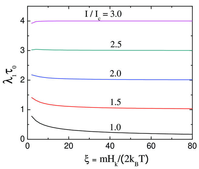
Figure 1:

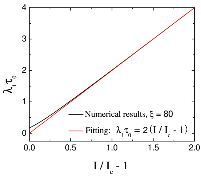
Figure 2:

References

- (1) J. Z. Sun et. al., Proc. SPIE Vol.5359, 445 (2004).
- (2) W. F. Brown, Jr., Phys. Rev. 130, 1677 (1963).
- (3) A. Aharoni, Phys. Rev. 177, 793 (1969).
- (4) C. N. Scully et. al., Phys. Rev. B 45, 474 (1992).
- (5) W. T. Coffey et. al., Phys. Rev. B 51, 15947 (1995);
- (6) X. Wang et. al., J. Appl. Phys. 92, 2064 (2002)
- (7) R. H. Koch et. al., Phys. Rev. Lett. 92, 088302 (2004)
- (8) Z. Li et. al., Phys. Rev. B 69, 134416 (2004);
- (9) D. M. Apalkov et. al., Phys. Rev. B 72, 180405(R) (2005)