On Statistics and 1/f Noise of Brownian Motion
in Boltzmann-Grad Gas and Finite Gas on Torus. II. Finite Gas

Abstract

An attempt is made to compare statistical properties of self-diffusion of particles constituting gases in infinite volume and on torus. In this second part, derivation, from BBGKY equations, of roughened model of self-diffusion is revised as applied to finite $N$-particle gas under micro-canonical ensemble. The model confirms existence of characteristic time $\approx N$, in units of free flight time, for cross-over between non-Gaussian and Gaussian regimes of diffusion, but then loses its legacy.

I Introduction

In the first part p1 of present work a most simplified version of the “collisional approximation” i1 of the Bogolyubov-Born-Green-Kirkwood-Yvon (BBGKY) equations was formulated and then used to analyze statistics of Brownian motion of gas particles in an infinite-volume gas under the Boltzmann-Grad limit ($\,\nu\rightarrow\infty\,$, $\,\delta\rightarrow 0\,$, $\,\lambda\sim 1/\nu\delta^{\mathcal{D}-1}=\,$const , where $\,\mathcal{D}\,$ is space dimension, $\,\nu\,$ and $\,\delta\,$ are concentration of gas particles and radius of their repulsive interaction, respectively, and $\,\lambda\,$ their mean free path). Now, our aim is to do something similar in respect to finite-volume gas on torus with finite total number of particles $\,N\,$.

Recall that the “collisional approximation” was introduced in i1 (one can see also i2 or Appendix B in p1 ) being mentioned as correct transition from exact BBGKY theory to Boltzmann-like theory in the case of spatially nonuniform gas, and in such sense it pretends to realization of earlier outspoken doubts about validity of the Boltzmann equation kac or, equivalently, provability of Boltzmann’s “Stosshalansatz” rdl in this case. One of key observations in i1 was that relative motion of colliding particles is inner constituent of their collision and therefore should be excluded from its outer characterization. In other words, probability density (ensemble-average concentration) of pair collisions $\,F_{2}\,$ undergoes an equation $\,\partial F_{2}/\partial t=-\bm{V}\cdot\partial F_{2}/\partial\bm{R}+...\,$, where $\,\bm{V}=(\bm{v}_{1}+\bm{v}_{2})/2\,$ and $\,\bm{R}=(\bm{r}_{1}+\bm{r}_{2})/2\,$ are velocity and position of the collision (more precisely, its center of gravity), and the dots replace “collision operators” acting onto the velocities. It is easy to prove that in actually nonuniform situation those $\,F_{2}\,$ (in contrary to general-position pair distribution function for non-colliding particles) can not be factored into product $\,F_{1}(t,\bm{r}_{1}\approx\bm{R},\bm{v}_{1})$$F_{1}(t,\bm{r}_{2}\approx\bm{R},\bm{v}_{2})\,$ of two one-particle distribution functions. Hence, it turns out to be independent supplementary characteristics of non-uniform gas.

If that is the case, then concentration $\,F_{3}\,$ of three-particle clusters, or “encounters” i1 , which enters the dots above, also is independent. It in its turn involves four-particle encounters, and so on. Thus we have to consider many coupled linear kinetic equations, which could be reduced to the single nonlinear Boltzmann equation under strict spatial uniformity only.

As in i1 (or i2 or p1 ) we will deal with not “thermodynamical” but “statistical” (“informational”) spatial non-uniformity implied by information about that (at some initial time moment $\,t=0\,$) one of gas particles is definitely positioned near some given place $\bm{r}=\bm{r}_{0}\,$. Corresponding (normalized to unit) distribution function of the whole gas can be chosen as

$$F_{N}(\bm{r},\bm{v})\,=\,F_{N}^{\,eq}(\bm{r},\bm{v})\,\frac{\Omega}{N}\,\sum_{j=1}^{N}\,\delta^{(\mathcal{D})}(\bm{r}_{j}-\bm{r}_{0})\,\,\,,\,\,\,\,\,\,\,$$ (1)

$$F_{N}^{\,eq}(\bm{r},\bm{v})\,=\,\frac{C_{N}(E)}{\Omega^{\,N}}\,\,\delta\left(E_{N}(\bm{r},\bm{v})\,-E\right)\delta^{(\mathcal{D})}\left(\sum_{j=1}^{N}\bm{v}_{j}\right)\,,$$

where $\,\Omega=l^{\mathcal{D}}\,$ is volume of gas contained in “flat cubic” torus $\,0\leq r_{\alpha}\leq l\,$ ($\,\alpha=1\div\mathcal{D}\,$), $\,E_{N}(\bm{r},\bm{v})\,$ is total energy of gas, and $\,F_{N}^{\,eq}(\bm{r},\bm{v})\,$ its equilibrium distribution with $\,C_{N}(E)\,$ being normalizing multiplier. Thus, unlike p1 , we will rest upon micro-canonical ensemble, with fixed total energy and zero total momentum, which looks natural at finite number of degrees of freedom.

We want to study consequent evolution of $\,F_{N}\,$ in order to obtain statistical characteristics of Brownian motion of initially localized particle. Unfortunately, direct solution of exact Liouville equation for $\,F_{N}\,$ is impossible. From the other hand, the Boltzmann equation (or, rather, Boltzmann-Lorentz equation rdl ) for $\,F_{1}\,$ can be easy solved, but in view of above reasonings (see i1 for detail discussion) it seems inadequate with respect to spatial dependence of $\,F_{1}\,$. Therefore by perforce we have to use the theory from p1 adapting it to finite system. At that, we can not exploit the Boltzmann-Grad limit which helps to obviate most of difficulties of the “collisional approximation” descending from vagueness of the very concept of “collision” i1 . By these reasons, at present only quite imperfect and caricature collisional model of nonuniform finite gas is available. Nevertheless, may be, it is better than uncritical use of the Boltzmann equation, all the more, better than nothing.

II Model equations

1.  Let us make non-principal assumptions as follow. First, of course, that total number of particles is large enough, $\,N\gg 1\,$. Second, mean free path is comparable with the torus dimensions: $\,\lambda\sim 1/\nu\delta^{\mathcal{D}-1}\sim l\,$, with $\,\nu=N/\Omega=N/l^{\mathcal{D}}\,$. Under these assumptions, estimate of a number of simultaneously occurring collisions obviously yields a value much smaller than unit: $\,N(\delta^{\mathcal{D}}N/\Omega)/2\,\sim\,N^{-1/(\mathcal{D}-1)}\,\ll 1\,$. Hence, our gas is sufficiently rarefied. On this ground, when considering probabilities of particle velocities, we can neglect potential energy contribution to $\,E_{N}(\bm{r},\bm{v})\,$ and write in (1) $\,E=N\mathcal{D}Mv_{0}^{2}/2\,$, with $\,v_{0}\,$ being characteristic velocity ($\,M\,$ is particle mass).

In order to get ability of watching for full rotations of particles around torus, let us use extended configurational space $\,-\infty<r_{\alpha}<\infty\,$, so that its cubic cell $\,(m_{\alpha}-1/2)l<r_{\alpha}<(m_{\alpha}+1/2)l\,$, with integer numbers $\,m_{\alpha}$, corresponds to $\,m_{\alpha}\,$ rotations along $\,\alpha$-th dimension during time period after $\,t=0\,$. Under this representation of life on torus, potential energy of interaction of any two particles changes to periodic function of coordinates, $\,U(\bm{\rho}(\bm{r}_{i}-\bm{r}_{j}))\,$, where $\,\bm{\rho}(\bm{r})\,$ means $\,\bm{r}\,$ modulo $\,l\,$: $\,\bm{\rho}_{\alpha}(\bm{r})\,$$=\bm{r}_{\alpha}-m_{\alpha}l\,$ when $\,(m_{\alpha}-1/2)l<r_{\alpha}<(m_{\alpha}+1/2)l\,$. At that, distribution (1) also will be extended to the whole space $\,-\infty<r_{\alpha}<\infty\,$, with $\,\Omega\,$ now being mentioned as its (infinite) volume. Such statistical ensemble implies, clearly, that rotations of only a sole (initially localized) particle will be watched, while getting of information about absolute positions and displacements of other particles is beforehand eliminated.

Next, consider particular $\,n$-particle distribution functions which follow from (1):

$$F_{n}(\bm{r}_{1}...\,\bm{v}_{n})\,=\,\int_{n+1}...\int_{N}F_{N}(\bm{r},\bm{v})\,=\,\,\,\,\,\,\,\,\,\,\,\,\,\,$$

$$=\,\frac{\Omega}{N}\,\,F_{n}^{\,eq}(\bm{r}_{1}...\,\bm{v}_{n})\sum_{j=1}^{n}\,\delta^{(\mathcal{D})}(\bm{r}_{j}-\bm{r}_{0})\,+\,\,\,\,\,\,\,$$ (2)

$$\,\,\,\,\,+\,\frac{(N-n)\,\Omega}{N}\,\int F_{n+1}^{\,eq}(\bm{r}_{1}...\,\bm{r}_{n},\bm{r}_{0},\bm{v}_{1}...\,\bm{v}_{n},\bm{v}^{\prime})\,d\bm{v}^{\prime}\,\,\,,$$

$$F_{n}^{\,eq}(\bm{r}_{1}...\,\bm{v}_{n})\,=\,\int_{n+1}...\int_{N}\,F_{N}^{\,eq}(\bm{r},\bm{v})\,\,\,,\,\,\,\,\,\,\,\,\,\,\,$$ (3)

where $\,\int_{s}...=\int...\,\,d\bm{v}_{s}d\bm{r}_{s}\,$. Since, according to (1), $\,F_{n}\sim\Omega^{-\,n}\,$, and $\,\Omega\,$ has become infinite, while $\,N\,$ is finite, it is evident that the second term on right-hand side of (2) factually vanishes in comparison with first term and should be thrown away when considering nonuniform (localized) parts of $\,F_{n}$’s. Besides, it is reasonable to move off also common multiplier $\,1/N\,$. Thus we can write

$$F_{n}(\bm{r}_{1}...\,\bm{v}_{n})\,=\,\Omega\,F_{n}^{\,eq}(\bm{r}_{1}...\,\bm{v}_{n})\,\sum_{j=1}^{n}\,\delta^{(\mathcal{D})}(\bm{r}_{j}-\bm{r}_{0})\,$$ (4)

with normalization $\,\int_{1}...\int_{n}\,F_{n}\,=\,n\,\Omega^{\,n-1}\,$.

2.  Formula (4), along with (1) and (3), presents initial conditions for the BBGKY equations

$$\frac{\partial F_{n}}{\partial t}\,=\,L^{(n)}F_{n}+(N-n)\int_{n+1}\sum_{j=1}^{n}L_{j\,n+1}F_{n+1}\,\,\,,$$ (5)

$$L^{(n)}\,=\,-\sum_{j=1}^{n}\bm{v}_{j}\cdot\frac{\partial}{\partial\bm{r}_{j}}\,+\sum_{1\leq\,i<j\,\leq n}L_{\,ij}\,\,\,,\,\,\,\,\,\,\,\,\,$$

$$\,\,\,\,\,\,L_{\,ij}\,=\,\nabla U(\bm{\rho}(\bm{r}_{i}-\bm{r}_{j}))\cdot\left(\frac{\partial}{\partial\bm{p}_{\,j}}-\frac{\partial}{\partial p_{i}}\right)\,\,\,\,\,\,\,\,\,\,\,\,\,\,$$

In “collisional approximation” we want to transform the right-hand integrals in (5) into Boltzmann-like “collisional integrals”.

This is possible in those cases only when statistical ensemble under consideration contains all various consecutive phases (instant dynamic states) of a collision process, moreover, when all that phases are represented by the ensemble with equal probability. Otherwise, the collision process can not be replaced by momentary collision event, since the latter must conserve probability (in essence, conserve particles). Of course, hardly a non-trivial ensemble ever (even at Bogolyubov’s “kinetic stage”) undergoes such requirement in formally rigorous sense. Therefore this requirement should be interpreted as instruction how to make “collisional approximation”.

Firstly, we must consider special values of $\,F_{n}\,$ ($\,n>1\,$) corresponding to clusters (“encounters” i1 ; i2 ) of $\,n\,$ mutually close particles (e.g. satisfying, in real torus space, conditions $\,|\bm{r}_{i}-\bm{r}_{j}|<d\,$, where $\,d\,$ is significantly smaller than $\,l\,$ but greater than $\,\delta\,$). At $\,n=2\,$ the matter concerns either literally collision or close encounter of two particles with no essential interaction, while at $\,n>2\,$ we speak about chains of close pair collisions or their combinations with mere encounters (in particular, might-have-been or “virtual” collisions in the sense mentioned in kac or rdl ).

Secondly, divide term $\,L^{(n)}F_{n}\,$ in (5) into two parts, one coming from non-uniformity of statistical ensemble, that is $\,F_{n}$’s dependence on translations $\,\bm{r}_{j}\rightarrow\bm{r}_{j}+\Delta\bm{r}\,$, and other from its dependence on dynamic phase of $\,n$-particle encounter. This can be done in the form

$$L^{(n)}F_{n}\,=-\bm{V}^{(n)}\cdot\sum_{j=1}^{n}\frac{\partial F_{n}}{\partial\bm{r}_{j}}-\frac{\partial F_{n}}{\partial\Theta}\,\,\,,$$ (6)

where $\,\bm{V}^{(n)}=(\bm{v}_{1}+...+\bm{v}_{n})/n\,$ is velocity of centroid of the $\,n$-particle cluster, and $\,\Theta\,$ is its inner time in the centroid’s reference frame. Obviously, $\,\sum\partial/\partial\bm{r}_{j}\,$ is just infinitesimal operator of plane-parallel displacement of the whole cluster. About $\,\Theta\,$ see i2 or Appendix B in p1 .

Thirdly, and chiefly, following the above requirement, second term in (6) must pass for zero: $\,\partial F_{n}/\partial\Theta\rightarrow 0\,$, since the concept of collisions imposes equiprobability of its dynamic phases (in particular, its border “in-” and “out-” states), i.e. conservation of probability.

After all, $\,F_{n}\,$, being taken at $\,|\bm{\rho}(\bm{r}_{i}-\bm{r}_{j})|<d\,$, becomes probabilistic characteristics of $\,n$-particle encounters as one-piece events. Two right-hand terms in (5) turn into drift and source of the encounters, respectively (to be precise, drift and source of their ensemble-average concentration). At that, the requirement $\,\partial F_{n}/\partial\Theta\rightarrow 0\,$ once again plays important role: it serves for transforming the source into sum of collision operators which act upon $\,F_{n+1}\,$ i1 ; i2 .

However, still $\,F_{n}\,$ possesses too many arguments (after removal of $\,\Theta\,$, only by unit less than generally), including impact parameters and other internal geometric details of an encounter. Therefore simultaneously let us exclude the latter arguments by averaging $\,F_{n}\,$ over them. Beforehand notice that spatial dependence of exact solution to (5) starting from (4) must look like

$$F_{n}\,=\,\widetilde{F}_{n}(t,\bm{r}_{1}\,;\,\bm{\rho}(\bm{r}_{2}-\bm{r}_{1}),...\,\bm{\rho}(\bm{r}_{n}-\bm{r}_{1}))+\,\text{CP}\,\,\,,$$ (7)

where $\,\widetilde{F}_{n}\,$ is symmetric with respect to indices $\,2\div n\,$ and “CP” means sum of $\,n-1\,$ cyclic permutations of all $\,n\,$ indices. For this reason, it is sufficient (with no loss of information) to average $\,F_{n}\,$ over only $\,\bm{r}_{j}\,$ belonging to one and the same cell of the extended space (and multiply results by some constants to keep suitable normalization).

Thus, fourthly, introduce $\,W(\bm{r})\,$ as some spherically symmetric bell-shaped (and normalized to unit) weighting function with width $\,\sim d\,$ (i.e. approximately enclosing a region assigned to collisions and encounters) and then averaged distributions as

$$\overline{F}_{n}\,=\,\Omega^{n-1}\int...\int F_{n}\,\prod_{j=1}^{n}W(\bm{r}_{j}-\bm{R})\,d\bm{r}_{j}\,\,\,$$ (8)

Applying such operation to (5), in view of (7), we can replace expressions $\,\int d\bm{r}_{n+1}\,U(\bm{\rho}(\bm{r}_{j}-\bm{r}_{n+1}))\,...\,$ by expressions $\,(\nu\,\Omega/N)\,\int d\bm{r}_{n+1}\,U(\bm{r}_{j}-\bm{r}_{n+1})\,...\,$ with $\,\Omega\,$ being (infinite) volume of the extended space and $\,\nu\,$ (real finite) concentration of gas. Taking into account also equalities (6) and $\,\partial F_{n}/\partial\Theta=0\,$, and manipulating by analogy with i1 ; i2 , it is not hard to obtain

$$\frac{\partial\overline{F}_{n}}{\partial t}=\,-\bm{V}^{(n)}\cdot\frac{\partial\overline{F}_{n}}{\partial\bm{R}}+\frac{N-n}{N}\,\sum_{j=1}^{n}\,S_{j\,n+1}\overline{F}_{n+1}^{\,in}\,$$ (9)

with $\bm{V}^{(n)}=n^{-1}\sum_{j\,=1}^{n}\bm{v}_{j}\,$ . Symbol $\,S_{j\,n+1}\,$ designates Boltzmannian linear collision operator describing collision between $\,j$-th member of $\,n$-particle cluster and an exterior $\,(n+1)$-th particle. The latter came from outside of the cluster and is in incoming state with respect to it, being placed somewhere at its border. Function $\,\overline{F}_{n+1}^{\,in}\,$ just represents such situation.

The last collision terms in (9) split to purely pair collisions (without participation of other members of a cluster at $\,n>2\,$). Strictly speaking, this statement is simply demonstrable only for infinite gas under the Boltzmann-Grad limit (when $\,d\,$ can be chosen so that $\,\delta/d\rightarrow 0\,$ despite $\,d/\lambda\rightarrow 0\,$ and any cluster becomes “infinitely rarefied from within” although“infinitely dense from without”). Nevertheless, even if it is formally wrong, in essence this is not significant defect of our model, because, as we will see, factual role of collisions is exchange between momentum of “outer $(n+1)$-th” particle and total momentum of $\,n$-particle cluster.

What is more important, we came to the point where, fifthly, we need in a hypothesis like Boltzmann’s Stosshalansatz (“molecular chaos”) in order to reduce functions $\,\overline{F}^{\,in}\,$ to functions $\,\overline{F}$ and thus close equations (9). But both trivial reasoning mentioned in the Introduction and deeper considerations i1 ; i2 show that it can not be literally Boltzmann’s hypothesis. If speak about infinite gas, nothing prevents a cluster’s (“$j$-th”) particle and exterior (“$(n+1)$-th”) particle be statistically independent in the sense of their velocities, but, naturally, their positions are statistically dependent, which is expressed by $\,\overline{F}_{n+1}^{\,in}(t,\bm{R},\bm{v}_{1}...\,\bm{v}_{n},\bm{v}_{n+1})$ $=\,F_{0}(\bm{v}_{n+1})$$\int\overline{F}_{n+1}(t,\bm{R},\bm{v}_{1}...\,\bm{v}_{n},\bm{v}^{\prime})\,d\bm{v}^{\prime}\,$ (with $\,F_{0}(\bm{v})\,$ being Maxwell distribution when gas is in thermodynamical equilibrium). However, in finite gas, framed by the micro-canonical ensemble (1), even velocities of “$j$-th” and “$(n+1)$-th” particle must be statistically dependent. In view of this new difficulty, relations of $\,\overline{F}_{n+1}^{\,in}\,$ to $\,\overline{F}_{n+1}\,$ will be analyzed in concrete way of further simplification of the model.

3.  According to (1), (4) and (8) and notions made in the beginning of this Section, initial conditions to equations (9) must be

$$\overline{F}_{n}(t=0,\bm{R},\bm{v}_{1}...\,\bm{v}_{n})\,=\,n\,W(\bm{R})\,\overline{F}_{n}^{\,eq}(\bm{v}_{1}...\,\bm{v}_{n})\,\,\,,$$ (10)

$$\overline{F}_{n}^{\,eq}(\bm{v}_{1}...\,\bm{v}_{n})\,=\,\int d\bm{v}_{n+1}\,...\int d\bm{v}_{N}\,\times\,\,\,\,\,\,\,\,\,\,\,\,\,\,\,\,$$

$$\times\,\,C_{N}(E)\,\delta\left(\frac{M}{2}\sum_{j\,=1}^{N}\bm{v}_{j}^{2}\,-E\right)\delta^{(\mathcal{D})}\left(\sum_{j\,=1}^{N}\bm{v}_{j}\right)\,\,\,,$$

where $\,E=N\mathcal{D}Mv_{0}^{2}/2\,$, we took $\,\bm{r}_{0}=0\,$, and $\,\overline{F}_{n}^{\,eq}\,$ are equilibrium velocity distributions normalized to unit. The integration yields

$$\overline{F}_{n}^{\,eq}\,\propto\left[\mathcal{D}Nv_{0}^{2}-\sum_{j\,=1}^{n}\bm{v}_{j}^{2}-\frac{\left(\sum_{j\,=1}^{n}\bm{v}_{j}\right)^{2}}{N-n}\right]^{(N-\,n-1)\mathcal{D}/2-\,1}$$

Soon we will use the first and second statistical moments of these distributions:

$$\langle\bm{v}_{j}\rangle\,=\,0\,\,,\,\,\,\,\langle v_{i\alpha}v_{j\beta}\rangle\,=\,v_{0}^{2}\,\delta_{\alpha\beta}\left[\delta_{ij}\,-\,\frac{1-\delta_{ij}}{N-1}\right]\,\,,$$ (11)

where $\,\langle\,[...]\,\rangle\,=\,\int...\int\,[...]\,\,\overline{F}_{n}^{\,eq}\,d\bm{v}_{1}...\,d\bm{v}_{n}\,$ and $\,i,j\leq n\,$, and besides the incomplete integral

$$\int\bm{v}_{n+1}\,\overline{F}_{n+1}^{\,eq}\,d\bm{v}_{n+1}\,=\,-\frac{\bm{v}_{1}+...\,+\bm{v}_{n}}{N-n}\,\,\overline{F}_{n}^{\,eq}\,\,$$ (12)

Obviously, factor $\,-(\bm{v}_{1}+...\,+\bm{v}_{n})/(N-n)\,$ here is nothing but conditional average value of $\,\bm{v}_{n+1}\,$ under fixed $\,\bm{v}_{j\leq n}\,$.

4.  As in p1 , mostly we are interested in spatial distributions and conjugated probability flows

$$W_{n}(t,\bm{R})\,=\int...\int\overline{F}_{n}(t,\bm{R},\bm{v}_{1}...\bm{v}_{n})\,d\bm{v}_{1}...\,d\bm{v}_{n}\,\,\,,$$

$$\bm{J}_{n}(t,\bm{R})\,=\int...\int\bm{V}^{(n)}\,\overline{F}_{n}(t,\bm{R},\bm{v}_{1}...\bm{v}_{n})\,d\bm{v}_{1}...\,d\bm{v}_{n}\,\,\,,$$

first of all, $\,W_{1}(t,\bm{R})\,$ which is probability density of random Brownian displacement of initially localized particle (from its start position near $\,\bm{R}=0\,$).

Similar to p1 , let us derive from (9) roughened but closed and solvable equations for these distributions, by using the fact that after a few collisions (counted off from $\,t=0\,$) cross-correlation between previously accumulated displacement $\,\bm{R}\,$ of Brownian particle and its current velocity $\,\bm{v}\,$ becomes small. Indeed, the conditional average value of $\,\bm{v}_{\alpha}\,$ at given $\,\bm{R}\,$ is $\,\approx R_{\alpha}/t\,$. Since $\,|\bm{R}_{\alpha}|\sim\sqrt{2Dt}=\sqrt{2v_{0}^{2}\tau_{f}t}\,$ (with $\,D\,$ being diffusivity and $\,\tau_{f}\sim\lambda/v_{0}\,$ mean free flight time), modulus of this average is $\,\sim v_{0}\sqrt{2\tau_{f}/t}\,$, hence already at $\,t\sim 20\tau_{f}\,$ it is small enough in comparison with magnitude $\,v_{0}\,$ of equilibrium velocity fluctuations.

At larger time the displacement-velocity cross correlation can be treated as a weak perturbation. Clearly, corresponding weakly perturbed distribution functions $\,\overline{F}_{n}\,$ can be written as

$$\overline{F}_{n}(t,\bm{R},\bm{v}_{1}...\bm{v}_{n})\,=\,\overline{F}_{n}^{\,eq}(\bm{v}_{1}...\,\bm{v}_{n})\,\times\,\,\,\,\,\,\,\,\,\,\,\,\,$$ (13)

$$\times\,\,[\,W_{n}(t,\bm{R})\,+\,\bm{w}_{n}(t,\bm{R})\cdot(\bm{v}_{1}+...\,+\bm{v}_{n})\,+...\,]\,\,\,,$$

where first term in squire brackets represents zero-order contribution from asymptotic with independent velocity and displacement, while the dots replace higher-order contributions. The latter will be neglected and omitted. Substituting (13) into definition of the flows and using (11) we find relations of $\,\bm{w}_{n}\,$ to them:

$$\bm{J}_{n}(t,\bm{R})\,=\,\frac{N-n}{N-1}\,v_{0}^{2}\,\bm{w}_{n}(t,\bm{R})\,\,$$ (14)

Next notice that the question about connections between distribution functions $\,\overline{F}_{n+1}^{\,in}\,$ and $\,\overline{F}_{n+1}\,$ will be simply resolved in the framework of the first-order approximation if we write

$$\overline{F}_{n+1}^{\,in}(t,\bm{R},\bm{v}_{1}...\,\bm{v}_{n+1})\,=\,\overline{F}_{n+1}^{\,eq}(\bm{v}_{1}...\,\bm{v}_{n+1})\,\times\,\,\,\,\,\,\,\,\,$$ (15)

$$\times\,\{\,W_{n+1}(t,\bm{R})+\bm{w}_{n+1}(t,\bm{R})\cdot a_{n}\,[\sum_{j\,=1}^{n}\bm{v}_{j}+c_{n}\bm{v}_{n+1}]\}$$

and choose coefficient $\,a_{n}\,$ and $\,c_{n}\,$ to be such that mean value of $\,\bm{v}_{n+1}\,$ turns into zero,

$$\int\bm{v}_{n+1}\,\overline{F}_{n+1}^{\,in}\,d\bm{v}_{1}...\,d\bm{v}_{n+1}=\,0\,\,\,,$$ (16)

while mean values of $\,\bm{v}_{j}\,$ with $\,j<n+1\,$ remain exactly the same as under distribution $\,\overline{F}_{n+1}\,$:

$$\int\bm{v}_{j}\,\overline{F}_{n+1}^{\,in}\,d\bm{v}_{1}...\,d\bm{v}_{n+1}=\int\bm{v}_{j}\,\overline{F}_{n+1}\,d\bm{v}_{1}...\,d\bm{v}_{n+1}\,$$

With the help of (11)-(12), these requirements yield

$$c_{n}\,=\,\frac{n}{N-1}\,\,\,,\,\,\,\,\,a_{n}\,=\,\frac{N-1}{N}\,\,\,,$$ (17)

respectively.

At such $\,a_{n}\,$ and $\,c_{n}\,$, expressions (15) and (16) say that velocity of outer $\,(n+1)$-th particle is not correlated with position of $\,n$-particle cluster it came in (as if it was a particle from equilibrium thermostat), although its position can be correlated (as if it was full member of greater $\,(n+1)$-particle cluster). This is just what is required by the “weakened molecular chaos” suggested in i1 ; i2 as a compromise of mutually contradicting “pure Stosshalansatz” and conservation of probabilities.

Consider time derivatives of the probability flows, combining (9) with expressions (13) and (15), noticing that

$$\langle\,V^{(n)}_{\alpha}V^{(n)}_{\beta}\rangle\,=\,\delta_{\alpha\beta}\,\frac{N-n}{n\,(N-1)}\,v_{0}^{2}\,$$ (18)

due to (11), and everywhere keeping only lowest-order nonzero contributions:

$$\frac{\partial\bm{J}_{n}}{\partial t}\,=\,-\,\frac{N-n}{n\,(N-1)}\,v_{0}^{2}\,\frac{\partial W_{n}}{\partial\bm{R}}\,+\,\,\,\,\,\,\,\,\,\,\,\,\,\,\,\,\,\,\,\,\,\,\,\,$$

$$+\,\frac{N-n}{N}\,a_{n}\int d\bm{v}_{1}...\int d\bm{v}_{n}\,\bm{V}^{(n)}\times\,\,\,\,\,\,\,\,\,\,\,\,$$ (19)

$$\,\,\,\,\times\,\,\bm{w}_{n+1}(t,\bm{R})\cdot\sum_{i\,=1}^{n}\,S_{\,i\,n+1}\,[\,\sum_{j\,=1}^{n}\bm{v}_{j}+c_{n}\bm{v}_{n+1}]\,\overline{F}_{n+1}^{\,eq}\,$$

Action of the collision operator is defined as usually,

$$S_{\,i\,n+1}\,f(...\,\bm{v}_{i}...\,\bm{v}_{n+1})\,=\,\nu\int db\int d\bm{v}_{n+1}\,\times\,\,\,\,\,\,\,\,$$

$$\times\,\,|\bm{v}_{i}-\bm{v}_{n+1}|\,[f(...\,\bm{v}_{i}^{\prime}...\,\bm{v}_{n+1}^{\prime})-f(...\,\bm{v}_{i}...\,\bm{v}_{n+1})]\,\,\,\,,$$

where $\,b\,$ is $\,(\mathcal{D}-1)$-dimensional impact parameter, and $\,\bm{v}_{i}^{\prime}=\,\bm{v}_{i}^{\prime}(\,\bm{v}_{i}\,,\bm{v}_{n+1},b)\,$ and $\,\bm{v}_{n+1}^{\prime}=\,\bm{v}_{n+1}^{\prime}(\,\bm{v}_{i}\,,\bm{v}_{n+1},b)\,$ are those in-state velocities which result in given out-state velocities $\,\bm{v}_{i}\,$ and $\,\bm{v}_{n+1}\,$ after collision. Taking into account that $\,\bm{v}_{i}+\bm{v}_{n+1}=\bm{v}_{i}^{\prime}+\bm{v}_{n+1}^{\prime}\,$ and $\,\overline{F}_{n+1}^{\,eq}\,$ are invariants of collision, it is easy to verify that

$$S_{\,i\,n+1}\,[\,\sum_{j\,=1}^{n}\bm{v}_{j}+c_{n}\bm{v}_{n+1}]\,\overline{F}_{n+1}^{\,eq}\,=-\frac{1}{2}\,(1-c_{n})\,\nu\times\,\,$$

$$\times\,\int db\int d\bm{v}_{n+1}[\,1-\cos\,\theta\,]|\bm{v}_{i}-\bm{v}_{n+1}|(\bm{v}_{i}-\bm{v}_{n+1})\overline{F}_{n+1}^{\,eq}$$

where $\,\theta=\theta(|\bm{v}_{i}-\bm{v}_{n+1}|\,,b)\,$ denotes scattering angle as a function of collision parameters. Of course, spherical symmetry of interaction potential was assumed. Now perform in (19) integrations first over all $\,\bm{v}_{j}\,$ with $\,j\neq i,n+1\,$, using relations similar to (12), and second over $\,\bm{v}_{i}\,$ and $\,\bm{v}_{n+1}\,$, paying attention to symmetry of resulting equations, and introduce the “relaxation rate”

$$\gamma\,=\,\frac{(N-1)\,\nu}{4Nv_{0}^{2}}\int d\bm{v}\int d\bm{v}^{\prime}\int db\,\,|\bm{v}-\bm{v}^{\prime}|^{3}\,\times$$

$$\times\,[\,1-\cos\,\theta(|\bm{v}-\bm{v}^{\prime}|\,,b)\,]\,\overline{F}_{2}^{\,eq}(\bm{v},\bm{v}^{\prime})\,$$

Finally, with the help of (14) and (17), equation (19) transforms to

$$\frac{\partial\bm{J}_{n}}{\partial t}\,=\,-\,\frac{v_{0}^{2}}{n}\,\frac{N-n}{N-1}\,\frac{\partial W_{n}}{\partial\bm{R}}\,-\,\gamma\,\frac{N-n}{N}\,\,\bm{J}_{n+1}\,\,\,,$$ (20)

It remains to supplement (20) by equations

$$\frac{\partial W_{n}}{\partial t}\,=\,-\,\frac{\partial\bm{J}_{n}}{\partial\bm{R}}\,\,\,,$$ (21)

and initial conditions

$$W_{n}(t=0,\bm{R})\,=\,n\,W(\bm{R})\,\,\,,\,\,\,\bm{J}_{n}(t=0,\bm{R})=0\,\,\,,$$ (22)

which directly follow from (9) and (10).

Clearly, $\,\gamma\,$ can be identified with inverse mean free flight time $\,1/\tau_{f}\,$. We may replace $\,W(\bm{R})\,$ by delta-function $\,\delta^{\mathcal{D}}(\bm{R})\,$, since anyway we have to consider spatial scales much greater then $\,d\,$. Of course, index $\,n\,$ in (20)-(22) takes values $\,1\leq n\leq N-1\,$, because zero total momentum in our micro-canonical statistical ensemble (1), (10) requires to set

$$\bm{J}_{N}(t,\bm{R})=0\,\,\,$$ (23)

The same is dictated by (14), (18) or (20) at $\,n=N\,$.

If we chose canonical ensemble, then in (16) we would have to write $\,c_{n}=0\,$ and $\,a_{n}=1\,$ in place of (17), while formulas (14) and (18) would change to $\,\bm{J}_{n}=v_{0}^{2}\bm{w}_{n}\,$ and $\,\langle V^{(n)}_{\alpha}V^{(n)}_{\beta}\rangle=\delta_{\alpha\beta}\,v_{0}^{2}/n\,$, resulting in

$$\frac{\partial\bm{J}_{n}}{\partial t}\,=\,-\,\frac{v_{0}^{2}}{n}\,\frac{\partial W_{n}}{\partial\bm{R}}\,-\,\gamma\,\frac{N-n}{N}\,\,\bm{J}_{n+1}\,\,\,,$$ (24)

instead of (20), now with $\,1\leq n\leq N\,$ and $\,\bm{J}_{N}\neq 0\,$.

III Model analysis

1.  First, as in p1 , consider solution to equations (20)-(22) in terms of Fourier and Laplace transforms

$$\Xi_{n}(t,\,\bm{k})\,=\,\int\exp(i\,\bm{k}\cdot\bm{r})\,W_{n}(t,\bm{r})\,d\bm{r}\,\,\,,$$

$$\Phi_{n}(p,\,\bm{k})\,=\,\int_{0}^{\infty}\exp(-p\,t)\,\,\Xi_{n}(t,\,\bm{k})\,dt\,\,$$

At that, in view of obvious isotropy of Brownian motion under interest, it is sufficient to watch for its projection onto some axis only, formally changing “wave vector” $\,\bm{k}\,$ by scalar $\,k\,$. Then

$$\Phi_{1}(p,k)=\,\frac{1}{p}\,+\sum_{n=1}^{\infty}\frac{(-k^{2})^{n}}{(2n)!}\int_{0}^{\infty}e^{-p\,t}\,\langle R^{2n}(t)\rangle\,dt\,$$

with $\,\langle R^{2n}(t)\rangle=\int R^{2n}\,W_{1}(t,R)\,dR\,$ being statistical moments of (a projection of) Brownian displacement.

Now from (20)-(22) we come to finite series:

$$p\,\Phi_{n}(p,\,k)\,-\,n\,=\,\frac{v_{0}^{2}k^{2}N}{p\,\gamma(N-1)}\,\times\,\,\,\,\,\,\,\,\,\,\,\,\,\,\,\,\,\,\,\,\,\,\,\,\,\,\,$$ (25)

$$\times\,\sum_{s\,=n}^{N-1}\prod_{m\,=n}^{s}\left[-\frac{(N-m)\gamma}{Np}\right]\left[1+\frac{v_{0}^{2}k^{2}(N-m)}{mp^{\,2}(N-1)}\right]^{-1}\,$$

Correspondingly, Laplace transform of $\,\langle R^{2n}(t)\rangle\,$ is $\,(2n+N-1)$-order polynomial of $\,1/p\,$ with powers from $\,2n+1\,$ to $\,2n+N-1\,$. Hence, $\,\langle R^{2n}(t)\rangle\,$ itself is $\,(2n+N-2)$-order polynomial of $\,t\,$ with powers from $\,2n\,$ to $\,2n+N-2\,$.

In particular,

$$\int_{0}^{\infty}e^{-p\,t}\langle R^{2}(t)\rangle\,dt=-\frac{2D}{p^{\,2}}\sum_{s=1}^{N-1}\frac{(N-1)!}{(N-s-1)!}\left(-\frac{\gamma}{Np}\right)^{s}$$

which means that

$$\frac{d}{dt}\,\langle R^{2}(t)\rangle=\,2D\left[\,1\,-\,\left(1-\frac{\gamma t}{N}\right)^{N-1}\right]\,$$ (26)

with diffusivity $\,D\,$ presented by

$$D\,=\,\frac{v_{0}^{2}N}{\gamma(N-1)}\,\,$$

Consider also fourth-order moment of (projection of) the displacement:

$$\int_{0}^{\infty}e^{-p\,t}\langle R^{4}(t)\rangle\,dt\,=\,-\,\frac{24D^{2}\gamma}{p^{\,4}}\,\times\,\,\,\,\,\,\,\,\,\,\,\,\,$$

$$\times\,\sum_{s=1}^{N-1}\frac{(N-1)!}{(N-s-1)!}\left(-\frac{\gamma}{Np}\right)^{s}\left[\,\sum_{m=1}^{s}\frac{1}{m}\,-\frac{s}{N}\right]$$

which yields in the time domain

$$\frac{d^{\,2}}{dt^{2}}\,\langle R^{4}(t)\rangle=\,24D^{2}\left(\,\vartheta^{N-1}-\frac{1}{N}-\frac{N-1}{N}\,\vartheta^{N}\right)\,+$$

$$+\,\,24D^{2}\sum_{s\,=1}^{N-1}\left(\frac{1-\vartheta^{\,s}}{s}-\frac{\vartheta^{\,s}-\vartheta^{N}}{N-s}\right)\,\,\,\,\,\,\,\,\,$$ (27)

with factor $\,\vartheta=\vartheta(t)\,$ defined by

$$\vartheta\,=\,1-\frac{\gamma t}{N}$$

Polynomials representing higher-order statistical moments may be considered in terms of functions $\,V^{(m)}_{n}(t)\,$ introduced by analogy with right-hand sides of (26)-(27):

$$2m\,\left(\frac{d\,}{dt}\right)^{m-1}\int R^{2m-1}\,J_{\,n}(t,R)\,dR\,=\,\,\,\,\,\,\,\,\,\,\,\,\,\,\,\,\,\,$$ (28)

$$=\,\left(\frac{d\,}{dt}\right)^{m}\int R^{2m}\,W_{n}(t,R)\,dR\,\equiv\,(2m)!\,D^{m}\,\,V^{(m)}_{n}(t)\,\,$$

From (20)-(22) recurrent equations for $\,V^{(m)}_{n}(t)\,$ directly follow:

$$\frac{dV^{(m)}_{\,n}}{dt}\,=\,\gamma\,\frac{N-n}{N}\left[\,\frac{1}{n}\,\,V^{(m-\,1)}_{n}\,-\,V^{(m)}_{n+1}\,\right]$$ (29)

with $\,1\leq n\leq N-1\,$, $\,V^{(0)}_{n}(t)\,=\,n\,$, $\,m\geq 1\,$, initial conditions $\,V^{(m)}_{n}(t=0)=0\,$, and $\,V^{(m)}_{N}=0\,$ because of (23). In particular, at $\,m=1\,$ equations (29) yield generalization of (26),

$$\frac{d}{dt}\int R^{2}\,W^{(1)}_{n}\,dR\,=\,2D\,\left[1-\vartheta^{N-\,n}\right]\,$$ (30)

2.  Expressions (26) and (27) look quite formally satisfactory and physically reasonable as long as $\,\gamma t<N\,$, that is $\,\vartheta>0\,$. Moreover, as it naturally might be expected, at sufficiently large $\,N\,$ and $\,1\ll\gamma t<N\,$ (more precisely, at $\,|\vartheta|^{N}<1\,$) they approximately coincide with expressions for infinite system p1 , that is $\,2D\,$ and $\,24D^{2}\,\ln\,\gamma t\,\,$, respectively (as the consequence, while $\,\gamma t<N\,$ the diffusivity $\,1/f$-noise exists in the sense explained in p1 ; i1 ). Similar statements are true also in respect to various higher moments $\,\int R^{2m}W_{n}(t,R)\,dR\,$ which follow from (25) or (29) and to the whole probability distribution functions $\,W_{n}(t,R)\,$ (at least at $\,N-n\gg 1\,$). Particular example is shown in Fig.1.

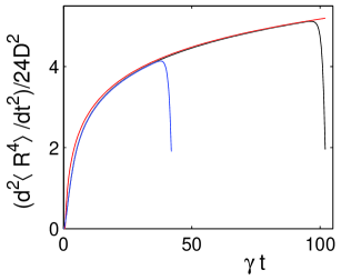
Figure 1: Plots of $\,(24D^{2})^{-1}\,d^{2}\langle R^{4}(t)\rangle/dt^{2}\,$ via $\,\gamma t\,$ corresponding to (27) at $\,N=21\,$ (blue) and $\,N=51\,$ (black) in comparison with $\,\ln{(\gamma t)}+C\,$ (red) which approximates limit $\,N\rightarrow\infty\,$ ($\,C\,$ is Euler constant).

However, at $\,\gamma t>N\,$ ($\,\vartheta<0\,$) the same expressions (26), (27) and (30) become obviously senseless. Notice that $\,\vartheta\,$ and its various powers $\,\vartheta^{\,s}\,$ play roles of relaxation factors being direct analogues, especially at $\,s\sim N\,$, of the exponent $\,\exp{(-\gamma t)}\,$ in infinite system. Therefore, negative $\,\vartheta\,$ with growing absolute value has none physical meaning.

Hence, we should conclude that solution to equations of our model (20)-(22) possesses peculiar time point $\,N/\gamma=N\tau_{f}\,$. Out of it the model does not work.

These fact can not be addressed to some incidental details of the model. Indeed, other model corresponding to canonical ensemble and represented by equations (24) in place of (20) possesses the same peculiar point. It is not hard to trace that the peculiarity arises from two things: presence of factor $\,N-n\,\,$ in collision term of equations (20) and characteristic open-chain structure of these equations with $\,n$-th member referring to $\,(n+1)$-th. Both have migrated from the basic BBGKY equations. But the second is also child of the “weakened molecular chaos” hypothesis. Hence, just the latter (to be precise, its concrete realization on the form of (15)-(16)) is responsible for the peculiarity.

It seems natural to interpret this situation as evidence that at $\,\gamma t=N\,$ period of non-Gaussian behavior of our random walk is over. Then predicted peculiar time $\,N/\gamma\,$ conceptually as well as numerically coincides with time $\,\tau_{ng}\,$ suggested in p1 as characteristic time scale separating “non-ergodic” (non-Gaussian) and “ergodic” (asymptotically Gaussian) stages of the walk.

3.  In order to construct a better model (where weakened molecular chaos would self-destruct with time into complete one) we should return to higher level of equations (9) or BBGKY equations. This is subject of separate investigation (principally, it is plausible if “trivial” Gaussian asymptotic creates nontrivial problems).

At present, we confine ourselves by discussion of most weak spot of the model. Undoubtedly, that is the “end cap” (23) which makes closure of the chain (20), but rather bad closure, because it means that $\,(N-1)$-particle cluster loses any interaction with rest $\,N$-th particle. Here is the reason to remove $\,(N-1)$-th of equations (20) from affected zone of the “weakened molecular chaos” hypothesis (16)-(17). Then it takes the form

$$\frac{\partial\bm{J}_{N-1}}{\partial t}=-\,\frac{v_{0}^{2}}{(N-1)^{2}}\,\frac{\partial W_{N-1}}{\partial\bm{R}}\,-\,\gamma\,\frac{1}{N}\,\widetilde{\bm{J}}_{N}\,\,\,,$$

$$\widetilde{\bm{J}}_{N}\,\equiv\,v_{0}^{2}\,a_{N-1}(1-c_{N-1})\,\bm{w}_{N}\,\,\,\,\,\,\,\,\,\,\,\,\,\,\,\,$$ (31)

Equality (23) remains true, but now it is out of work. The model becomes temporarily non-closed, and we get chance to correct its behavior after $\,t\sim\tau_{ng}\,$ (notice that $\,\tau_{ng}\,$ is just time necessary to transfer influence by $\,\widetilde{\bm{J}}_{N}\,$ from last to first of equations (20)).

Let us demonstrate that in presence of $\,\widetilde{\bm{J}}_{N}\,$ the model comprises Gaussian asymptotic at $\,t/\tau_{ng}\rightarrow\infty\,$, moreover, without significant assumptions about accompanying asymptotic of $\,\widetilde{\bm{J}}_{N}\,$. According to (28), Gaussian asymptotic means that $\,V^{(m)}_{1}(t\rightarrow\infty)\rightarrow 1\,$. Then other variables in equations (29) also have fixed points fully determined by $\,V^{(m)}_{1}(\infty)\,$ (as combined with $\,V^{(0)}_{n}=n\,$):

$$V^{(m)}_{n}(\infty)\,=\,\left\{\begin{array}[]{ll}(n-m)!/(n-1)!&\hbox{,}\,\,\,\,1\leq m<n\\ V_{1}^{(m-\,n\,+1)}(\infty)/(n-1)!&\hbox{,}\,\,\,\,m\geq n\end{array}\right.\,\,$$

Here $\,1\leq n\leq N\,$, and quantities $\,V_{N}^{(m)}(t)\,$ represent $\,\widetilde{J}_{N}(t,R)\,$ by the common rule (28) with $\,n=N\,$ and $\,\widetilde{J}_{N}(t,R)\,$ in place of $\,J_{N}(t,R)\,$. We did not fulfil substitution $V^{(m)}_{1}(\infty)=1$. This helps to visualize that $V^{(m)}_{N}(\infty)$ at least at $m<N$ appear insensible to $V^{(m)}_{1}(\infty)$ (i.e. independent on assumption about gaussianity of the asymptotic) thus justifying above statement. Notice also that equalities $V^{(m)}_{1}(\infty)=1$ imply equalities $\,V^{(m)}_{2}(\infty)=V^{(m)}_{1}(\infty)\,$ (at $m>0$), which mean that asymptotically $\,J_{2}(t,R)\rightarrow J_{1}(t,R)\,$ and therefore first pairs of equations (20)-(21) stands apart, as it must be in standard kinetics.

IV Conclusion

In the first part of this paper p1 a simple kinetic model of self-diffusion (Brownian motion) in infinite-volume gas was developed. It exploits collisional description of interaction between particles but declines Boltzmann’s “molecular chaos” hypothesis because the latter appears incompatible with two doubtless theoretical requirements to be fulfilled: probability conservation during collisions and necessity to deal with spatially nonuniform statistical ensemble when considering random walks of gas particles. Instead, the “weakened molecular chaos” hypothesis suggested in i1 was used, which is consistent with both the requirements and claims statistical independency of colliding particles in respect to their velocities only but not their coordinates. It resulted in a chain of kinetic equations whose solution shows that statistics of random walks of gas particles does not obey the law of large numbers and remains essentially non-Gaussian at arbitrary long time scales, including what can be named 1/f fluctuations in diffusivity.

Physical origin of so wild statistical freedom is absence of actual cause-and-effect correlations between successive fragments of the random walk, in spite of statistical long-living correlations formally describing the same freedom i1 ; i2 . Its mathematical origin is absence of relaxation (in the ordinary sense) terms in kinetic equations. Usual place of relaxation terms is occupied by references to next higher-order equations. This chain of references mean that a particle whose random walk is under observation constantly accumulates (actual) correlations with more and more new particles.

In infinite gas this process lasts endlessly. In finite $\,N$-particle gas it ends at time $\sim N$ (counted from start of the observation, in units of mean free flight time) when collisions of observed particle with all others have realized, therefore, initial conditions of the whole system have snapped into action. Further motion of this particle is fully predestined by already observed walk, representing its reflections (mappings) in complete non-decaying actual correlation with all the gas. This creates the necessary prerequisites for decay of statistical correlations between particles and realization of the law of large numbers and Gaussian statistics at next longer time scales.

The model investigated in this second part of the paper certainly detects time $\approx N$ of this transition but, unfortunately, is unfit for description of the next Gaussian asymptotic of the random walk. However, in principle, the exact BBGKY equations give a firm base for proper improving the model. From the other hand, practically sooner just the former non-Gaussian stage is of interest, since $N$ means rather large time. In this respect, the model needs in improvements too. Probably, at present form it somehow overestimates “degree of non-gaussianity” of the random walk. The early phenomenological construction of “quasi-Gaussian” walk bk3 (see also references therein and i2 ) produced much softer non-gaussianity (although also with 1/f noise in diffusivity). In any case, there are many interesting questions for future.

References

• (1) Yu. E. Kuzovlev, β€œOn statistics and 1/f noise of Brownian motion in Boltzmann-Grad gas and finite gas on torus. II. Infinite gas”, arXiv: cond-mat/0609515.
• (2) Yu. E. Kuzovlev, β€œBBGKY equations, self-diffusion and 1/f-noise in a slightly nonideal gas”, Sov.Phys.-JETP, 67 (12), 2469 (1988) [in Russian: Zh.Eksp.Teor.Fiz., 94, No.12, 140 (1988)].
• (3) Yuriy E. Kuzovlev, β€œKinetical theory beyond conventional approximations and 1/f-noise”, arXiv: cond-mat/9903350.
• (4) M. Kac, β€œProbability and related topics in physical sciences”, Intersci. Publ., London, N.-Y., 1957.
• (5) P. Resibois and M. de Leener. Classical kinetic theory of fluids. Wiley, New-York, 1977.
• (6) G. N. Bochkov and Yu. E. Kuzovlev, β€œNew in 1/f-noise studies”, Sov.Phys.-Usp., 26, 829 (1983) [in Russian: UFN, 141, 151 (1983)].