Sampling the two-dimensional density of states $g(E,M)$ of a giant magnetic molecule using the Wang-Landau method

Abstract

The Wang-Landau method is used to study the magnetic properties of the giant paramagnetic molecule {Mo₇₂Fe₃₀} in which 30 Fe³⁺ ions are coupled via antiferromagnetic exchange. The two-dimensional density of states $g(E,M)$ in energy and magnetization space is calculated using a self-adaptive version of the Wang-Landau method. From $g(E,M)$ the magnetization and magnetic susceptibility can be calculated for any temperature and external field.

I INTRODUCTION

During the past decade the field of molecular magnets has experienced a rapid evolution.Gatteschi et al. (1994); Caneschi et al. (1999); Gatteschi et al. (2006) Nowadays a vast variety of species can be synthesized, ranging in size from 2 to more than 30 paramagnetic ions embedded in the host molecule.Müller et al. (1998) The fascinating properties of these new materials include hysteretic behavior,Caneschi et al. (1999); Chiorescu et al. (2000); Waldmann et al. (2002) quantum tunneling of the magnetization,Thomas et al. (1996); Friedman et al. (1996); Gatteschi and Sessoli (2003) magnetocaloric,Waldmann et al. (2002); Schnack (2006) and magnetostrictive effects.Schnack et al. (2006)

Astonishingly, for several observables and not too low temperatures it is sufficient to treat magnetic molecules classically by applying the Heisenberg model.Müller et al. (2001) This enables one to apply the powerful machinery of classical stochastic sampling methods. The Metropolis algorithm Metropolis et al. (1953) has become the standard tool to calculate statistical classical properties of these nano magnets.Schröder et al. (2005a, b) Recently, the Wang-Landau algorithmWang and Landau (2001a) (WL) has been successfully applied to various problems in statistical physics and biophysics both to models with discrete Wang and Landau (2001a, b) as well as with continuous degrees of freedom.Kim et al. (2006); Rathore et al. (2004); Yan and de Pablo (2003); Zhou et al. (2006a) In this context the WL exhibits a superior feature in comparison to the Metropolis algorithm. Since the WL calculates the density of states (DOS), one can estimate thermodynamic observables such as the free energy and entropy for all temperatures using just one single simulation of the density of states.

However, the calculation of the DOS in energy space $g(E)$ permits only to calculate thermodynamic properties as a function of temperature and at zero magnetic field, e.g. the zero-field specific heat, but not observables such as the magnetic susceptibility at non-vanishing field.Brown and Schulthess (2005) For studying the magnetic properties of a system at arbitrary external magnetic field one has to calculate a joined DOS $g(E,M)$ in energy and magnetization space. Once $g(E,M)$ is known, properties like magnetization $M$ and magnetic susceptibility $\chi$ can be calculated at any temperature and any external magnetic field using again just one single simulation of the density of states.Zhou et al. (2006a, b)

In this article we introduce a self-adaptive version of the WL which allows to calculate the two-dimensional DOS $g(E,M)$ using a discrete binning scheme in the continuous energy and magnetization space. We demonstrate that the WL is capable to calculate efficiently all thermodynamic properties of rather large spin systems using the example of the magnetic Keplerate molecule {Mo₇₂Fe₃₀}.Müller et al. (1999) The dependencies of the thermodynamic observables both on temperature and external magnetic field can be obtained by only one single simulation. We conclude by discussing the problems arising at low temperatures and high magnetic fields.

II MODEL AND COMPUTATIONAL METHODS

In the Keplerate molecule {Mo₇₂Fe₃₀} 30 iron (III) ions ($s=5/2$) occupy the vertices of a perfect icosidodecahedron,Müller et al. (1999) see Fig. 1. The spins are coupled with their nearest neighbors by an isotropic and antiferromagnetic coupling of strength $J/k_{B}=1.566$ K. The spectroscopic splitting factor is $g=1.974$.Müller et al. (2001)

Figure 1: Geometrical structure of an icosidodecahedron. For the molecule {Mo₇₂Fe₃₀} the vertices represent spin sites and the edges represent nearest neighbor interactions.

We write the Heisenberg Hamiltonian as

$$H=J\sum_{\langle m,n\rangle}\mathbf{S}_{m}\cdot\mathbf{S}_{n}+g\mu_{B}{B}^{(z)}\cdot\sum_{n}{S}^{(z)}_{n}\ ,$$ (1)

whereas $\langle m,n\rangle$ directs that the sum is over distinct nearest-neighbor pairs, ${B}^{(z)}$ is an external magnetic field in $z$-direction, $\mu_{B}$ is the Bohr magneton, and $\mathbf{S}$ denotes classical vectors of length $|\mathbf{S}|=\sqrt{(s(s+1))}$.Luscombe et al. (1998) We use a self-adaptive Troster and Dellago (2005) scheme of the WL to calculate the two-dimensional DOS $g(E,M)$, where $E$ denotes the Heisenberg energy of a given spin configuration of Hamiltonian (1) without external magnetic field, i.e.

$$E=J\sum_{<m,n>}\mathbf{S}_{m}\cdot\mathbf{S}_{n}\ ,$$ (2)

and $M$ is the magnetization in $z$-direction, which is defined as the sum over the $z$-components of all classical spin vectors:

$$M=\sum_{n}{S}^{(z)}_{n}\ .$$ (3)

In contrast to the Metropolis algorithm, where the acceptance probability of a new generated state is determined by $\min\{\exp[-(E_{j}-E_{i})/(k_{\mathrm{B}}T)],1\}$, the WL is characterized by an acceptance ratio $\min\{g(E_{j})/g(E_{i}),1\}$, where $E_{i}$ and $E_{j}$ refer to energies before and after the transition. The original WL has been applied to models where the energy assumes only discrete values.Wang and Landau (2001a, b) Since the Heisenberg model consists of classical spin vectors which are continuously orientable, the possible energy and magnetization values are real numbers between the minimum and maximum energy and magnetization, respectively. Thus, we discretize the continuous energy and magnetization range by the introduction of bins.Brown and Schulthess (2005); Zhou et al. (2006a) We have chosen bins of uniform width of $(\Delta E)/k_{\mathrm{B}}=4$ K in energy and $\Delta M=0.6\cdot|\mathrm{S}|$ in magnetization range. To speed up the simulation we divide the total energy range in eight overlapping intervals and follow the recipe in Ref. Schulz et al., 2003 to avoid boundary effects. A priori it is not known, which magnetization bins are accessible by the random walker in a certain energy interval. A striking feature of the WL is, that one does not have to know anything about the DOS one wants to calculate. Following the original WL, the random walker biases itself to explore the accessible energy and magnetization space. To do so, we have chosen the following procedure: At the beginning we perform a trial run for the desired energy interval. We introduce an initial DOS $g_{initial}(E,M)=1$ and a reference histogram $RH(E,M)$, and perform spin flips according the original WL procedure accepting and neglecting new spin configurations for a defined number of Monte-Carlo steps $n^{MC}_{initial}$. One Monte-Carlo step corresponds to a single spin tilt event. Each time a bin ($E_{i},M_{i}$) is visited the corresponding entries in $RH(E_{i},M_{i})=RH(E_{i},M_{i})+1$ and $g_{initial}(E_{i},M_{i})=f\cdot g_{initial}(E_{i},M_{i})$ are updated, whereas $f$ is the initial modification factor. Following this recipe the random walker triggers itself to explore the accessible energy and magnetization space for a predefined energy interval.

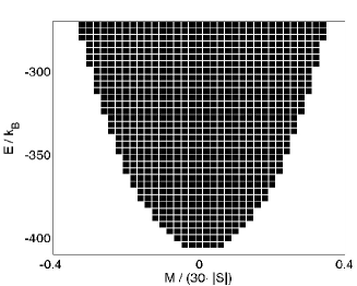
Figure 2: Low-energy part of the two dimensional map for the reference histogram with $RH(E,M)\neq 0$ for the molecule {Mo₇₂Fe₃₀}. $RH(E,M)\neq 0$ defines the accessible energy and magnetization space. The grid shows the bins in energy and magnetization space.

After $n^{MC}_{initial}$ steps have been performed we stop the initial run. Now we continue with the normal WL for the same energy interval. As an initial guess for the DOS we use $g_{initial}(E,M)$. A new state is only accepted if the corresponding entry in $RH(E,M)$ is not zero, compare Fig. 2. In other words, we accept only states corresponding to bins in the energy and magnetization space which have already been visited during the initial run, otherwise the new generated state is neglected according to Ref. Schulz et al., 2003. In addition, the relative flatness of the accumulated histogram is only checked after all valid entries in the reference histogram have been visited at least one hundred times. Of course the total runtime of the simulation as well as the accuracy of the finally calculated DOS are very sensitive to a good choice of $n^{MC}_{initial}$. If $n^{MC}_{initial}$ is chosen very large, the random walker explores bins at the boundaries of the accessible energy and magnetization space, which are rarely visited. Thus the DOS for these entries is small and does not contribute significantly to the partition function. Nevertheless, sampling of these states increases the total runtime of the simulation since a flat histogram is to be accumulated during the simulation. On the other hand, if $n^{MC}_{initial}$ is chosen too small, the energy and magnetization space is sparsely explored and many bins of the accessible energy and magnetization space are not visited, resulting in an inaccurate estimate of the DOS. Thus, the question is to find a good tradeoff between runtime and accuracy of $g(E,M)$. To estimate a reasonable value for $n^{MC}_{initial}$ for each energy interval, we have chosen different values and counted the number of visited distinct bins in $RH(E,M)$ after finishing the initial run. It turns out that the number of visited bins shows some saturation behavior. After a critical number of steps the visited energy and magnetization space does not grow significantly any more. Thus, after this critical number of steps has been reached we consider the accumulated $RH(E,M)$ to be a good estimate for the successive WL run. As the initial modification factor $f$ we have chosen a rather large value of $f_{start}=e^{4}$ and reduce $f$ in large steps.Zhou and Bhatt (2005) After finishing the initial run we perform 14 steps decreasing $f$ according to the recipe $f_{i+1}=\sqrt[4]{f_{i}}$ resulting in a final modification factor of 1.000000015. After $g(E,M)$ has been obtained, the magnetization $M(T,B)$ as a function of temperature $T$ and external magnetic field $B$ can be calculated from

$$\langle M(T,B)\rangle=\frac{\sum_{E,M}Mg(E,M)\exp(-H/k_{\mathrm{B}}T)}{\sum_{E,M}g(E,M)\exp(-H/k_{\mathrm{B}}T)}.$$ (4)

The differential magnetic susceptibility $\chi=\partial\langle M\rangle/{\partial B}$ can be computed by using the equation

$$\chi(T,B)=\frac{1}{k_{\mathrm{B}}T}[\langle M^{2}(T,B)\rangle-\langle M(T,B)\rangle^{2}].$$ (5)

While without external magnetic field it is sufficient to calculate only the DOS for negative energies, since states with positive energies due to their Boltzmann factor $\exp(-E/k_{\mathrm{B}}T)$ practically do not contribute to the partition function, in the case of an external magnetic field also energy bins with a positive energy become important, since they might be low-lying in the case of an applied external field. Thus it is required to calculate the DOS over the full energy range of the system, if the properties at high magnetic fields are studied. The exact ground state energy for {Mo₇₂Fe₃₀} is known to be $E_{0}/k_{\mathrm{B}}=-412.125$ K,Axenovich and Luban (2001) which is close to the lowest accessible energy bin of $E_{min}/k_{\mathrm{B}}=-406$ K. The classical ground state of the molecule is charactereized by relative angles of 120^∘ between nearest-neighbor spins.Axenovich and Luban (2001) The possibility of generating such a spin configuration is practically zero, and thus an effective sampling of the DOS near the ground state energy is not possible. The same is valid for the highest energy states of the molecule, where the probability of generating a spin configuration with all spins pointing in the same direction is unlikely. The highest energy bin visited during the initial run is $E_{max}/k_{\mathrm{B}}=786$ K. As the criterion of flatness we used a relatively small value of 0.5, and to further decrease the statistical error we perform four runs, calculate the magnetic properties for each of these runs and compute the mean value and mean standard deviation afterwards. On a personal computer (Intel, Xeon, 2.60 GHz) the sampling of the complete DOS took about 120 hours of cpu time.

For a comparison of accuracy we performed extensive Monte-Carlo simulations using the Metropolis algorithm. We perform $30\cdot 10^{6}$ spin tilt trials to let the system reach equilibrium at a defined external magnetic field and temperature. Afterwards for additional $30\cdot 10^{6}$ tilting trials the thermodynamic properties are computed.

III RESULTS AND DISCUSSION

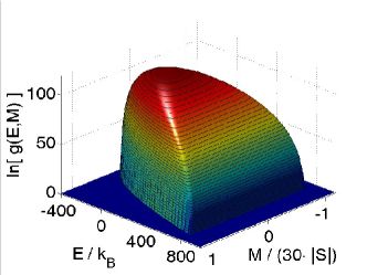
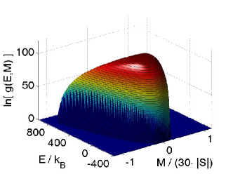
Figure 3: (Color online) Joint DOS $\ln[g(E,M)]$ for the magnetic molecule {Mo₇₂Fe₃₀}.

The calculated joint DOS $g(E,M)$ for the magnetic molecule {Mo₇₂Fe₃₀} is presented in Fig. 3. One notices that the low-energy boundary $E_{\text{min}}(M)$ assumes a parabolic shape as observed for various systems.Waldmann (2001); Schnack and Luban (2001) The region with $\partial g(E,M)/\partial M=0$ at high energies indicates the global rotational symmetry of the system. One also notices that in the vicinity of the phase-space boundary the classical density of states grows very rapidly by orders of magnitude which explains why it is difficult to obtain very accurate results at the boundaries.

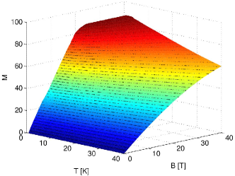
Figure 4: (Color online) Magnetization $M$ as a function of temperature $T$ and external magnetic field $B$.

The limited accuracy at the energy and magnetization space boundaries looses its significance with increasing temperature. This is demonstrated by evaluating the magnetization as a function of temperature $T$ and external magnetic field $B$. Figure 4 shows the behavior of the magnetization in the relevant temperature and field range. The simulated magnetization does not show any significant statistical fluctuations; it compares nicely to the result of a Metropolis sampling.

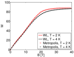
Figure 5: (Color online) Comparison of the magnetization $M$ as a function of external magnetic field calculated from $g(E,M)$ (solid lines) with computed data using the Metropolis algorithm at $T=2$ K (open circles) and 4 K (open squares), respectively. Statistical sampling errors are smaller than the used symbols and line widths.

Figure 5 compares the magnetization at $T=2$ K and 4 K as a function of field for the WL and the Metropolis simulations. As can be inferred from the figure, at a temperature of the order of the exchange coupling the WL reaches the same accuracy as the Metropolis algorithm, but the latter has to be performed for each pair of variables $(T,B)$, whereas with the WL the density of states has to be sampled only once in order to obtain the complete function $\langle M(T,B)\rangle$.

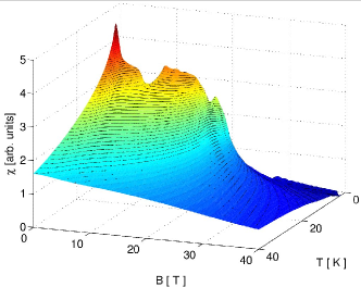
Figure 6: (Color online) Magnetic susceptibility $\chi$ as a function of temperature $T$ and external magnetic field $B$.

Figure 7: (Color online) Comparison of the magnetic susceptibility $\chi$ as a function of external magnetic field calculated from $g(E,M)$ (solid lines) with computed data using the Metropolis algorithm at $T=2$ K (open circles) and 4 K (open squares), respectively.

The differential susceptibility, Figs. 6 and 7, is a second derivative of the partition function. Therefore, it will magnify inaccuracies of the simulated density of states. Figure 6 displays the susceptibility as a function of $T$ and $B$. It can be seen that for temperatures higher than $J/k_{B}$ the behavior is rather smooth, but for lower temperatures a spiky behavior is observed which results from statistical fluctuations at the energy and magnetization space boundary. At $T\approx J/k_{B}$ these fluctuations are still visible, but on average much smaller than the real minimum at about $B_{\text{sat}}/3$,Schröder et al. (2005a) compare Fig. 7. Clearly one can see that the dip in suszeptibility at about $B_{\text{sat}}/3$ vanishes with increasing temperature.Schröder et al. (2005a) The spurious peak at $T=0$ and $B=0$ reflects the difficulty to obtain the density of states in close vicinity of the ground state. A comparison with Metropolis simulations is shown is Fig. 7. The results obtained using both methods agree well. The fluctuations in the WL data are due to the missing bins in $g(E,M)$ at the energy and magnetization space boundaries, since these features are apparent in all four WL runs. The statistical sampling errors are given by the size of the symbols and by the line widths used in Fig. 7.

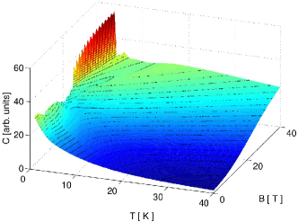
Figure 8: (Color online) Specific heat $C$ as a function of temperature $T$ and external magnetic field $B$.

The last function we want to discuss in this paper is the specific heat $C$ as a function of temperature $T$ and external magnetic field $B$. As can be seen in Fig. 8 the specific heat does not show too strong fluctuations at low temperature and fields below saturation. It seems that this observable is more robust against statistical fluctuations of the density of states than the susceptibility. In order to complete the discussion we display the specific heat also for magnetic fields above the saturation field where it shows strong fluctuations. They reflect magnified inaccuracies at the high energy boundary of $g(E,M)$ and thus are spurious.

Summarizing, one can say that the proposed self-adaptive version of the Wang-Landau algorithm can efficiently generate the density of states $g(E,M)$ of a rather large spin system, such as the magnetic molecule {Mo₇₂Fe₃₀}. The obvious advantage is that with one simulation of $g(E,M)$ many thermodynamic observables can be evaluated as function of temperature and applied magnetic field. Statistical fluctuations are apparent in the second derivatives of the two-dimensional DOS, namely the specific heat and magnetic suszeptibility at low temperatures. These fluctuations can be minimized at the cost of computational time, by either increasing the number of bins or by a more strict flatness criterion. Recently, it was demonstrated that a fitting of the one-dimensional DOS for a sampled energy interval by higher order polynomials results in a less fluctuating specific heat.Parsons and Williams (2006) Nevertheless, it is stated, that this fitting procedure fails if one tries to extrapolate the DOS outside the sampled energy interval using the fitting function. Thus, further improvements are still needed to provide an effective sampling at the boundaries of $g(E,M)$. Due to the fact that the density of states varies by many orders of magnitude it is clear that close to the boundaries of $g(E,M)$ the statistics becomes poorer.

References

- Gatteschi et al. (1994) D. Gatteschi, A. Caneschi, L. Pardi, and R. Sessoli, Science 265, 1054 (1994).
- Caneschi et al. (1999) A. Caneschi, D. Gatteschi, C. Sangregorio, R. Sessoli, L. Sorace, A. Cornia, M. A. Novak, C. Paulsen, and W. Wernsdorfer, J. Magn. Magn. Mater. 200, 182 (1999).
- Gatteschi et al. (2006) D. Gatteschi, R. Sessoli, and J. Villain, Molecular Nanomagnets, Mesoscopic Physics and Nanotechnology (Oxford University Press, Oxford, 2006).
- Müller et al. (1998) A. Müller, F. Peters, M. Pope, and D. Gatteschi, Chem. Rev. 98, 239 (1998).
- Chiorescu et al. (2000) I. Chiorescu, W. Wernsdorfer, A. Müller, H. Bögge, and B. Barbara, Phys. Rev. Lett. 84, 3454 (2000).
- Waldmann et al. (2002) O. Waldmann, R. Koch, S. Schromm, P. Müller, I. Bernt, and R. W. Saalfrank, Phys. Rev. Lett. 89, 246401 (2002).
- Thomas et al. (1996) L. Thomas, F. Lionti, R. Ballou, D. Gatteschi, R. Sessoli, and B. Barbara, Nature 383, 145 (1996).
- Friedman et al. (1996) J. R. Friedman, M. P. Sarachik, J. Tejada, and R. Ziolo, Phys. Rev. Lett. 76, 3830 (1996).
- Gatteschi and Sessoli (2003) D. Gatteschi and R. Sessoli, Angew. Chem., Int. Edit. 42, 268 (2003).
- Schnack (2006) J. Schnack, J. Low. Temp. Phys. 142, 279 (2006).
- Schnack et al. (2006) J. Schnack, M. Brüger, M. Luban, P. Kögerler, E. Morosan, R. Fuchs, R. Modler, H. Nojiri, R. C. Rai, J. Cao, et al., Phys. Rev. B 73, 094401 (2006).
- Müller et al. (2001) A. Müller, M. Luban, C. Schröder, R. Modler, P. Kögerler, M. Axenovich, J. Schnack, P. C. Canfield, S. Bud’ko, and N. Harrison, Chem. Phys. Chem. 2, 517 (2001).
- Metropolis et al. (1953) M. Metropolis, A. Metropolis, M. Rosenbluth, A. Teller, and E. Teller, J. Chem. Phys. 21, 1087 (1953).
- Schröder et al. (2005a) C. Schröder, H. Nojiri, J. Schnack, P. Hage, M. Luban, and P. Kögerler, Phys. Rev. Lett. 94, 017205 (2005a).
- Schröder et al. (2005b) C. Schröder, H. J. Schmidt, J. Schnack, and M. Luban, Phys. Rev. Lett. 94, 207203 (2005b).
- Wang and Landau (2001a) F. Wang and D. P. Landau, Phys. Rev. Lett. 86, 2050 (2001a).
- Wang and Landau (2001b) F. Wang and D. P. Landau, Phys. Rev. E 64, 056101 (2001b).
- Kim et al. (2006) J. G. Kim, J. E. Straub, and T. Keyes, Phys. Rev. Lett. 97, 050601 (2006).
- Rathore et al. (2004) N. Rathore, Q. L. Yan, and J. J. de Pablo, J. Chem. Phys. 120, 5781 (2004).
- Yan and de Pablo (2003) Q. L. Yan and J. J. de Pablo, Phys. Rev. Lett. 90, 035701 (2003).
- Zhou et al. (2006a) C. G. Zhou, T. C. Schulthess, S. Torbrügge, and D. P. Landau, Phys. Rev. Lett. 96, 120201 (2006a).
- Brown and Schulthess (2005) G. Brown and T. C. Schulthess, J. Appl. Phys. 97, 10E303 (2005).
- Zhou et al. (2006b) C. G. Zhou, T. C. Schulthess, and D. P. Landau, J. Appl. Phys. 99, 08H906 (2006b).
- Müller et al. (1999) A. Müller, S. Sarkar, S. Q. N. Shah, H. Bogge, M. Schmidtmann, S. Sarkar, P. Kögerler, B. Hauptfleisch, A. X. Trautwein, and V. Schunemann, Angew. Chem. Int. Ed. Engl. 38, 3238 (1999).
- Luscombe et al. (1998) J. H. Luscombe, M. Luban, and F. Borsa, J. Chem. Phys. 108, 7266 (1998).
- Troster and Dellago (2005) A. Troster and C. Dellago, Phys. Rev. E 71, 066705 (2005).
- Schulz et al. (2003) B. J. Schulz, K. Binder, M. Müller, and D. P. Landau, Phys. Rev. E 67, 067102 (2003).
- Zhou and Bhatt (2005) C. G. Zhou and R. N. Bhatt, Phys. Rev. E 72, 025701(R) (2005).
- Axenovich and Luban (2001) M. Axenovich and M. Luban, Phys. Rev. B 63, 100407(R) (2001).
- Waldmann (2001) O. Waldmann, Phys. Rev. B 65, 024424 (2001).
- Schnack and Luban (2001) J. Schnack and M. Luban, Phys. Rev. B 63, 014418 (2001).
- Parsons and Williams (2006) D. F. Parsons and D. R. M. Williams, Phys. Rev. E 74, 041804 (2006).