Langevin simulations of a model for ultrathin magnetic films

Abstract

We show results from simulations of the Langevin dynamics of a two-dimensional scalar model with competing interactions for ultrathin magnetic films. We find a phase transition from a high temperature disordered phase to a low temperature phase with both translational and orientational orders. Both kinds of order emerge at the same temperature, probably due to the isotropy of the model Hamiltonian. In the low temperature phase orientational correlations show long range order while translational ones show only quasi-long-range order in a wide temperature range. The orientational correlation length and the associated susceptibility seem to diverge with power laws at the transition. While at zero temperature the system exhibits stripe long range order, as temperature grows we observe the proliferation of different kinds of topological defects that ultimately drive the system to the disordered phase. The magnetic structures observed are similar to experimental results on ultrathin ferromagnetic films.

I Introduction

In the last years the interest in understanding the thermodynamic and mechanical properties of magnetic ultrathin films has grown considerably. Part of this interest is obviously motivated by the great amount of technological applications related to their magnetic behavior, such as data storage and electronics Hubert and Schafer (1998). In recent years the advance in experimental techniques has made possible to study in great detail the complexity of magnetic order in thin films, where an extremely rich phenomenology is present Portmann et al. (2003); Wu et al. (2004); Jagla (2004). Part of this phenomenology - as in many other physical and chemical systems Seul and Andelman (1995) - is due to the presence of competing interactions acting on different length scales that frustrate the system and leads to mesoscopic pattern formation. In the case of an ultrathin magnetic film in the absence of an external magnetic field, stripe patterns of opposed magnetization are formed due to the competition between the ferromagnetic exchange interaction and the long-ranged dipolar interaction Garel and Doniach (1982).

Of particular interest for applications in data storage are films with strong perpendicular anisotropy, where spins point preferentially out of the plane. This happens when the (perpendicular) anisotropy energy overcomes the effect of dipolar interactions which induce an in-plane anisotropy. When this happens the system goes through a “spin reorientation transition” (SRT) Allenspach et al. (1990); Politi (1998); MacIsaac et al. (1998). In this phase, when magnetization points preferentially out of plane, complex magnetic structures arise, showing the formation of patterns with stripe order Vaterlaus et al. (2000); Portmann et al. (2003); Wu et al. (2004). Antiferromagnetic stripe order dominates the low temperature/low energy behavior. As temperature increases towards the SRT, perfect stripe order is disrupted by proliferation of topological defects, like dislocations and disclinations in the magnetic patterns, which eventually drive the system to the paramagnetic high temperature phase. Understanding how magnetic stripe order emerges from microscopic interactions and the characterization of the relevant thermodynamic behavior in the perpendicular phase is of relevance both from a fundamental point of view and for future applications in magnetic memory devices at the nanoscopic level.

Theoretical analysis of thermodynamic behavior rely on elastic Hamiltonian approximations and show a variety of possible scenarios, strongly dependent on the behavior of different kind of anisotropies present in the elastic energy Garel and Doniach (1982); Abanov et al. (1995); Politi (1998). In Abanov et al. (1995) two possible scenarios were anticipated, in one there is a single phase transition from a high temperature paramagnetic phase to a smectic (stripe) phase at low temperatures. Other possible scenario shows the presence of an intermediate nematic phase, where translational order is lost but orientational one persists. Searching for evidence of these scenarios is one of our motivations for the present work. There is also a rather large number of numerical simulations and analysis of the different patterns observed in ultrathin film models. Relevant to the present work are a series of simulations by MacIsaac and coworkers De’Bell et al. (2000). They made detailed Monte Carlo simulations of Heisenberg and Ising systems with competing exchange and dipolar interactions. The stripe nature of the ground state in a two dimensional system of Ising spins was determined analytically in MacIsaac et al. (1995). Phase diagrams showing the presence of the spin reorientation transition in Heisenberg models with perpendicular anisotropy, dipolar interactions and with or without exchange interactions were also studied MacIsaac et al. (1996, 1998). Cannas and coworkers have made a series of detailed predictions on phase diagrams and dynamic properties of a two dimensional Ising model with competing exchange and dipolar interactions Gleiser et al. (2002); Cannas et al. (2004, 2006) by Monte Carlo simulations. In particular, in Cannas et al. (2006) evidence was presented of a new, intermediate, nematic phase between the stripe and disordered phases. There is also a rather large amount of numerical work focused on qualitative descriptions of patterns, but few quantitative approaches.

Simulations of Heisenberg models have been largely restricted to determinations of phase diagrams mainly because analyzing quantitatively the structure of phases and patterns that emerge is a computationally very hard task in these models. On the other hand, studies of Ising models have also concentrated on quantitatively determining phase diagrams and also the presence and evolution of magnetic patterns. Nevertheless in the Ising case the sharp nature of domain walls induces a rather artificial structure of patterns, where e.g. tetragonal symmetry dominates completely the scene in square lattices. In this work we introduce a model intended to make a bridge between the more realistic but cumbersome Heisenberg models and the much simpler Ising models which nevertheless are not suitable for understanding the diversity of magnetic structures present in a real ultrathin film. Our results are qualitative in the sense that we do not intend to reproduce experimental parameter values of a particular system, but nevertheless we present a quantitative picture of phase transitions and the behavior of relevant thermodynamic variables in the regime of perpendicular magnetization, which can be easily mapped to real situations. Furthermore, the model introduced below admits numerical as well as analytical treatment of both equilibrium and dynamical behaviors and a comprehensive picture is beginning to emerge Barci and Stariolo ; Mulet and Stariolo (2007).

With this aim, in the present work we introduce and analyze, by means of Langevin simulations, a coarse grained model of an ultrathin film in two dimensions. By making reasonable approximations to the full micromagnetic dynamics, which should be satisfactory in the perpendicular region, we address the existence of antiferromagnetic stripe order, how thermal fluctuations affect this order, the possible appearance of a phase transition at finite temperature, and the characterization of the magnetic structures relevant in each temperature region. Coarse-grained models similar to the one introduced in the next section have been studied in the past. In an early work, Roland and Desai Roland and Desai (1990) studied the dynamical process of phase separation and emergence of stripe order in Langevin simulations of a model for ultrathin films. More recently, Jagla Jagla (2004) explored the different morphologies and patterns that can appear in such systems, showing a variety of very interesting phenomena. Furthermore, he showed that the same model is capable of reproducing the detailed phenomenology of histeretic behavior known in ultrathin films Jagla (2005). Nevertheless, up to our knowledge, more quantitative studies of the phase transitions and the different kinds of magnetic order present in these type of models have not been addressed up to now.

II Model and Numerical implementation

A widely acceptable microscopic description of micromagnetic dynamics is given by the Landau-Lifshitz-Gilbert equation Hubert and Schafer (1998):

$$\frac{\partial\vec{\phi}}{\partial t}=-\alpha\ \vec{\phi}\times\vec{B}-\gamma\ \vec{\phi}\times(\vec{\phi}\times\vec{B})$$ (1)

where $\vec{\phi}$ is the three dimensional magnetic moment vector, $\vec{B}$ is the effective field acting on it and $\alpha$ and $\gamma$ are microscopic phenomenological constants. The first term induces a precessional movement of the magnetic moment around the field, while the second term is a phenomenological one representing a damping effect which induces the magnetization to align with the field. This representation of magnetic dynamics is satisfactory in a wide variety of situations but it is very difficult to analyze analytically and is also very demanding computationally. Nevertheless, below the SRT where perpendicular anisotropy dominates, one can obtain a much simpler description of magnetization dynamics suitable to our purposes. Considering a single moment $\vec{\phi}$ with the effective field $\vec{B}$ pointing in the z direction and expanding the three components of $\vec{\phi}$ in eq.(1), one easily finds that the evolution of the perpendicular component is given by Jagla (2005):

$$\frac{\partial\phi_{z}}{\partial t}=\gamma\,B\ (1-\phi_{z}^{2})$$ (2)

where the constraint $\phi_{x}^{2}+\phi_{y}^{2}+\phi_{z}^{2}=1$ was used (this is automatically satisfied by the LLG dynamics). Then, in the limit of strong perpendicular anisotropy, when the effective field can be approximated to point preferentially along the z direction, the evolution of the perpendicular component is approximately autonomous, although the other two components are not. Consequently from now on we will restrict the analysis to the z component and drop out the corresponding subindex.

In the system of interest, the effective field will be composed typically of three contributions of the form:

$$B=h+a\ \phi-b\int d^{2}\mathbf{x^{\prime}}\ J(|\mathbf{x}-\mathbf{x^{\prime}}|)\ \phi(\mathbf{x^{\prime}})$$ (3)

where $h$ is an external field, the second term is a perpendicular anisotropy field and the last term will be the dipolar field in our case. The constants can be easily related with experimental ones, but this is not necessary for the purposes of this work, which is to study some universal properties of the phases and patterns emerging in such a system.

The complete energy function of the model consists of both a local and a nonlocal terms:

$$H[\phi]=H_{L}[\phi]+H_{NL}[\phi]$$ (4)

According to (3) for the case of zero external field, the local potential can be written in full generality:

$$H_{L}[\phi]=\frac{1}{2}\int d^{2}\mathbf{x}\big{[}\kappa(\bm{\nabla}\phi(\mathbf{x}))^{2}-r\phi^{2}(\mathbf{x})+\frac{u}{2}\phi^{4}(\mathbf{x})\big{]}$$ (5)

In order that the local potential assume the desired double-well structure, $u$ and $r$ are taken to be positive phenomenological constants. We have also added a continuous approximation for the exchange interaction in the form of an attractive square gradient term, which favors spatial homogeneity of the order parameter.

Disregarding higher order interactions in (3), the nonlocal term modeling a repulsive dipolar interaction has the form:

$$H_{NL}[\phi]=\frac{1}{2\delta}\int d^{2}\mathbf{x}\int d^{2}\mathbf{x^{\prime}}\phi(\mathbf{x})J(|\mathbf{x}-\mathbf{x^{\prime}}|)\phi(\mathbf{x^{\prime}})$$ (6)

where $J(|\mathbf{x}-\mathbf{x^{\prime}}|)=1/|\mathbf{x}-\mathbf{x^{\prime}}|^{3}$ in two dimensions. In equations (5) and (6), $\kappa$ and $\delta$ are positive phenomenological constants that describe, respectively, the range of the short-range exchange interaction and the strength of the long-range dipolar one. In all space integrations it is assumed a short distance cutoff $2\pi/\Lambda$, which in the numerical implementation appears naturally as the lattice constant $a$.

Hence, in the limit of strong perpendicular anisotropy and strong damping, the relaxational dynamics of the system can be modeled by the following Langevin equations:

$$\frac{{\partial\phi(\mathbf{x},t)}}{\partial t}=-\Gamma\frac{{\delta H[\phi]}}{\delta\phi(\mathbf{x},t)}+\eta(\mathbf{x},t)$$ (7)

where $\Gamma$ is a constant (the mobility) which sets the time scale, and $\eta(\mathbf{x},t)$ is a Gaussian thermal noise with $\left\langle\eta(\mathbf{x},t)\right\rangle=0$ and $\left\langle\eta(\mathbf{x},t)\eta(\mathbf{x}^{\prime},t^{\prime})\right\rangle=2\,\Gamma\,T\,\delta(t-t^{\prime})\,\delta^{2}(\mathbf{x}-\mathbf{x^{\prime}})$, as usual. Equation (7) can be explicitly written as:

$$\frac{1}{\Gamma}\frac{{\partial\phi(\mathbf{x},t)}}{\partial t} = \kappa\,\nabla^{2}\phi(\mathbf{x},t)+r\phi(\mathbf{x},t)-u\phi^{3}(\mathbf{x},t)$$

$$- \frac{{1}}{\delta}\int d^{2}\mathbf{x^{\prime}}\phi(\mathbf{x^{\prime}},t)J(|\mathbf{x}-\mathbf{x^{\prime}}|)+\eta(\mathbf{x},t)/\Gamma$$

It is convenient to express the above equations in dimensionless form by means of a transformation of variables. Following Roland and Desai Roland and Desai (1990), this transformation leads to the dimensionless form of equation (II):

$$\frac{{\partial\phi(\mathbf{x},t)}}{\partial t} = \nabla^{2}\phi(\mathbf{x},t)+\phi(\mathbf{x},t)-\phi^{3}(\mathbf{x},t)$$ (9)

$$- \frac{{1}}{\delta}\int d^{2}\mathbf{x^{\prime}}\phi(\mathbf{x^{\prime}},t)J(|\mathbf{x}-\mathbf{x^{\prime}}|)+\eta(\mathbf{x},t)$$

with a short distance cutoff $2\pi/\Lambda$ and thermal noise correlation $\left\langle\eta(\mathbf{x},t)\eta(\mathbf{x}^{\prime},t^{\prime})\right\rangle=2T\,\delta(t-t^{\prime})\,\delta^{2}(\mathbf{x}-\mathbf{x^{\prime}})$. Now the parameter $\delta$ stands for the relative strength between the two competing interactions. The last Langevin equation can be written in Fourier space as:

$$\frac{\partial\phi(\mathbf{k},t)}{\partial t}=-A(k)\phi(\mathbf{k},t)+\left[-\phi^{3}(\mathbf{x},t)+\eta(\mathbf{x},t)\right]_{\mathbf{k}}^{F}$$ (10)

To be compatible with the subsequent numerical implementation of this equation, the last two terms were not explicitly written in Fourier space. Here $\big{]}_{\mathbf{k}}^{F}$ means the ${\mathbf{k}}$ component of the corresponding Fourier transform. The function $A(k)$ corresponds to:

$$A(k)=k^{2}-1+J(k)/\delta$$ (11)

which encodes all spatial information about the interactions. If this quantity has a negative minimum at a wave vector $k_{m}$, selected by varying $\delta$, the solution of equation (10) is a modulation in a single direction with periodicity given by $k_{m}$.

We have numerically solved the stochastic differential equation (10) discretizing space in a square lattice with mesh size $a$. Periodic boundary conditions were implemented using the Ewald summation technique Frenkel and Smith (1996) in the long-range dipolar interaction. After spatial discretization this interaction is no longer isotropic for all spatial scales and it becomes gradually anisotropic as the wave vector comes close to $\pi$. At the relevant spatial scales for our simulations, $J(\mathbf{k})$ is slightly anisotropic. It is important to note that symmetry properties of the different magnetic structures appearing at low temperatures are affected by the square symmetry of the lattice. In a triangular lattice, for example, the phenomenology may be to some extent different Vedmedenko et al. (1998).

We found it advantageous to use a spectral method, since in the Fourier space form of the Langevin equation (10) both spatial derivatives and the dipolar interactions acquire an algebraic form.

The time derivative was approximated using a simple Euler scheme with a time step $\Delta t$. Taking an isotropic form of the discretized laplacian, the spatial derivatives were treated using a semi-implicit method, where the $k^{2}$ term in (10) is evaluated in the new time value. This treatment is standard to improve the stability of the algorithm Press et al. (1992).

Therefore, discretizing equation (10) in such manner, i.e. through a first order semi-implicit spectral method, we obtain the following recurrence relation:

$$\phi(\mathbf{k},t+\Delta t) = \frac{1}{1+\Delta t\,k^{2}}\{\left[1+\Delta t-\Delta t\,a^{2}J(\mathbf{k})/\delta\right]\phi(\mathbf{k},t)$$ (12)

$$+\left[-\Delta t\,\phi^{3}(\mathbf{x},t)+\eta(\mathbf{x},t)\right]_{\mathbf{k}}^{F}\,\}$$

After discretization the noise term $\eta$, in the way it appears in the last equation, is a random Gaussian number with amplitude $\left(2T\Delta t/a^{2}\right)^{1/2}$. The dipolar interaction $J(\mathbf{k})$ in (12) is the fast Fourier transform of the result of the Ewald summation, evaluated at the beginning of the simulation.

The computational advantage of updating the system in Fourier space is accomplished using an adaptative FFT algorithm Frigo and Johnson (2005), where the main time consuming operations are transforming Fourier the field $\phi$ and the $(-\phi^{3}+\eta)$ term and then transforming back the new field value.

III Results

We performed simulations of the continuum dipolar model through equation (12). We analyzed the case $\delta=2\sqrt{5}$, where the ground state is a stripe modulated state with wave vector $k_{m}=1.01447$, which is close to $\pi/3$. Simulations were performed for system sizes $L=192$ and $L=384$ for different temperatures.

The existence of a nontrivial solution with wave vector $k_{m}$ of the Langevin equation (10) at zero temperature depends on whether the term in (11) is negative at $k=k_{m}$. Before the variables transformation, this could be done varying the parameter $r$. After the transformation, the existence of a solution is achieved only by tuning the mesh size $a$. We set $a=\sqrt{5}$. The time integration was stable inside the range of temperatures of the simulations using a time step $\Delta t=0.5$.

To measure the orientational order of the stripes we first consider the director field:

$$\hat{n}(\mathbf{x})=\frac{\bm{\nabla}\phi(\mathbf{x})}{|\bm{\nabla}\phi(\mathbf{x})|}$$ (13)

which provides the local orientation of the stripe, when localized on a domain wall between opposite magnetizations. An analogy between this quantity and the Frank director of smectic liquid crystals has already been made on previous works Toner and Nelson (1981); Christensen and Bray (1998); Qian and Mazenko (2003), and leads to the definition of a tensor order parameter:

$$Q_{\alpha\beta}(\mathbf{x})=n_{\alpha}(\mathbf{x})n_{\beta}(\mathbf{x})-\frac{1}{2}\,\delta_{\alpha\beta}$$ (14)

where $\alpha,\beta=1,2$ are the cartesian components. Similar to a nematic order parameter in a liquid crystal, an orientational order parameter $Q$ can be defined as the positive eigenvalue of the spatial average of the above tensor order parameter Cuesta and Frenkel (1990). This value corresponds to the quantity $\cos 2\theta$, where $\hat{n}=(\cos\theta,\sin\theta)$ and $\theta$ is the angle between the local director field and the mean orientation of the system. But, since the director field inside the stripe domains does not necessarily provide the local orientation of the stripe, to get a more precise value for the orientational order parameter we average Eq.(14) only over domain wall sites, namely:

$$\overline{Q}_{\alpha\beta}=\frac{1}{L^{\prime}}\sum_{\mathbf{x}}\!^{\prime}\,Q_{\alpha\beta}(\mathbf{x})$$ (15)

where the prime denotes the restricted sum with $L^{\prime}$ being the total number of domain wall sites. Now we can write explicitly the orientational order parameter as:

$$Q=\sqrt{\overline{Q}_{11}^{\>2}+\overline{Q}_{12}^{\>2}}$$ (16)

One possible way to characterize the translational order of the stripes is through a staggered magnetization, defined as:

$$m_{\mathbf{k}}=\left<\frac{1}{L^{2}}\sum_{\mathbf{x}}sgn\left(\phi(\mathbf{x})\right)sgn\left(\cos(\mathbf{k}\cdot\mathbf{x})\right)\right>$$ (17)

where $sng$ is the sign function and for $\mathbf{k}$ we use the ground state wave vector.

The results we present here were obtained with the following procedure: the system is initialized in the ground state and heated with a heating rate $d_{T}$. At each temperature of interest, the heating process is halted and the system is left to run a transient period of $n_{t}$ time steps before we start recording system configurations at each $n_{m}$ time steps, used later to measure the desired quantities. Typical values of $n_{t}$ were between $5\times 10^{4}$ to $4\times 10^{6}$ in order to get as close as possible to equilibrium. To estimate both transient ($n_{t}$) and decorrelation ($n_{m}$) times we analyzed the behavior of the two-times correlation function for the different system sizes and temperatures. Typical $n_{m}$ values were in the order of $10^{5}$ and the results are averages over 20 to 60 system configurations.

Figure 1: Order parameters as a function of temperature for $L=192$. The open symbols corresponds to the larger system size, $L=384$. Thin vertical lines separate approximately temperature ranges of the different regimes.

In Fig. 1 we show the results for the translational and orientational order parameters. The data clearly shows a phase transition, where both kinds of order emerge at a finite temperature. In the $L=192$ case we found that the two order parameters decay simultaneously to zero at $T\approx 0.12$, even though the staggered magnetization drops significantly at $T=0.11$. In the region in between the translational order parameter seems to present strong finite size effects. As the temperature is lowered in the ordered phase, a stripe structure develops gradually by the annihilation of defects (see Fig. 3). Although we were unable to study in more detail the finite size scaling near the transition, it seems improbable that an intermediate, nematic-like phase, with only orientational order can be present in this model. Although translational order decays faster than the orientational one, our results point to the presence of a single phase transition from a disordered high temperature phase to a low temperature phase with both orientational and translational orders. This is one of the possible scenarios that emerge from a theoretical analysis of a similar model by Abanov et al.  Abanov et al. (1995).

To take a closer look at the structural properties of the different magnetic configurations, we calculated the static structure factor:

$$S(\mathbf{k})\equiv\left<\left|\phi(\mathbf{k})\right|^{2}\right>$$ (18)

and the associated spatial correlation function, given by:

$$C(\mathbf{r})=\frac{1}{L^{2}}\sum_{\mathbf{k}}e^{i\mathbf{r}\cdot\mathbf{k}}S(\mathbf{k}),$$ (19)

that can be quickly computed using a fast Fourier transform Frigo and Johnson (2005). The relevant directions for the spatial correlation function are the directions parallel and perpendicular to the stripes, respectively denoted by $C_{x}$ and $C_{y}$. This quantities describe the translational order along the two relevant directions. We have also computed nematic (or orientational) correlation functions Christensen and Bray (1998); Qian and Mazenko (2003), since they encode information on the spatial decay of orientational order of the stripes. Nematic correlations are defined as:

$$C_{nn}(\mathbf{r}) = \frac{2}{L^{2}}\sum_{\mathbf{x}}\left<\mathrm{Tr}\,\,Q(\mathbf{x}+\mathbf{r})Q(\mathbf{x})\right>$$ (21)

$$= \frac{1}{L^{2}}\sum_{\mathbf{x}}\left<Q_{11}(\mathbf{x}+\mathbf{r})Q_{11}(\mathbf{x})\right.$$

$$+\left.Q_{12}(\mathbf{x}+\mathbf{r})Q_{12}(\mathbf{x})\right>$$

where the function summed up in Eq. (21) is analogous to $\left<\cos\left[2\theta(\mathbf{x}+\mathbf{r})-2\theta(\mathbf{x})\right]\right>$. Examples of translational and orientational correlation functions can be seen in Figs. 2 and 4 for two different temperatures.

Figure 2: Correlation functions in the smectic-like region at $T=0.1$. The upper figure shows the connected orientational correlation function in the perpendicular direction for $L=384$, plotted in log-log scale, before and after the smoothing procedure. The continuous line corresponds to a fitting by the function $Ar^{-\alpha_{y}}$, with $\alpha_{y}=1.18$ and $A$ a fitting parameter. In the parallel direction this function decays immediately to zero. The lower figure shows the parallel (inset) and perpendicular spatial correlations functions, both for $L=192$. The parallel $C_{x}$ function is plotted in a log-log scale. The continuous lines corresponds to fittings by the functions $r^{-\omega_{x}}$ and $\cos(k_{0}r)r^{-\omega_{y}}$ with $\omega_{x}=0.33$ and $\omega_{y}=0.19$ and $k_{0}=1.014$. Similar values where found in the $L=384$ case.

For low enough temperatures ($T<0.11$), the nematic correlations are strongly affected by residual oscillations of the field $\phi(\mathbf{x})$. In order to obtain accurate values for the orientational correlation function we found convenient to smooth the tensor order parameter (14) following a smoothing procedure introduced in Ref.Qian and Mazenko (2003). We smooth the fields $Q_{11}(\mathbf{x})$ and $Q_{12}(\mathbf{x})$ using for each the iterative process:

$$f_{(n+1)}(\mathbf{x})=\frac{1}{2}f_{(n)}(\mathbf{x})+\frac{1}{8}\sum_{\mathbf{x}^{\prime}\in NN}f_{(n)}(\mathbf{x}^{\prime})$$ (22)

where $f_{(n)}$ is one of the fields after $n$ iterations, and $NN$ means the four nearest neighbors of $\mathbf{x}$ on the square lattice. We found that three iterations are enough to get sensible results (see Fig.2). Similar smoothing procedures for orientational correlation functions were used in simulations of melting of two-dimensional solid systems Lin et al. (2006); Jaster (1999). For clarity, in this work we always show the connected orientational correlation function, where the mean square orientational order parameter is substracted from Eq.(21). In this way, $C_{nn}$ accounts for direction fluctuations only.

At sufficiently low temperatures ($T<0.03$) spatial correlations decay immediately to a constant and there is translational and orientational long-range order (see Fig. 1 for the values of the order parameters in the corresponding temperature regimes).

(a)                                    (b)
 

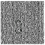
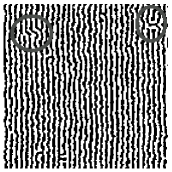
Figure 3: Typical configurations in the smectic phase for $L=192$ at (a) $T=0.1$ and (b) $T=0.104$. In (a) the encircled region exhibits two pairs of dislocations; above there is a ”passage” due to two dislocations inserted in the same stripe, and below a pair of dislocations separated by one stripe. In (b) a pair separated by four stripes and a pair formed by a larger Burgers vector dislocation and a double dislocation.

At slightly higher temperature and in a wide range ($0.03<T<0.11$) we found evidence of a low temperature smectic-like regime, similar to the smectic crystal phase predicted by Abanov et al. Abanov et al. (1995) and observed experimentally by Portmann et al. Portmann et al. (2003). In this phase, undulation fluctuations (meandering excitations) alone are sufficient to cause algebraic decay of translational correlations at low temperatures for $T>0.03$. But at $T=0.09$ bound pairs of dislocations appear and become more common as temperature increases. Long-range orientational order persists over a wider range of temperatures, but above $T=0.065$ orientational order also starts to decay algebraically.

An example of the algebraic behavior of the correlation functions in this region is shown in Fig. 2 for $T=0.1$. It is important to note that the exponent of the translational algebraic decay in this regime increases with temperature and is different in the perpendicular and parallel directions - exponents values range from $\omega_{x}=0.034$ and $\omega_{y}=0.036$ for $T=0.035$ to $\omega_{x}=0.365$ and $\omega_{y}=0.212$ for $T=0.104$. As for the orientational order we observe a small temperature dependence of the algebraic decay exponent in the perpendicular direction, with exponents lying in the range $1.18<\alpha<1.43$. In the parallel direction, the orientational correlation function is a constant, indicating long-range order in this direction.

In Fig. 3 we illustrate some typical configurations of this phase. We see that it is characterized by undulation excitations and a finite density of dislocation pairs - some different types are shown encircled.

Figure 4: Correlation functions in the nematic-like region at $T=0.114$ and $L=384$. The upper figure shows the connected orientational correlation function in the perpendicular and parallel directions in a log-linear scale. The continuous lines corresponds to fittings by the function $A\exp(-r/\lambda)$, with $\lambda_{y}=13.77$ and $\lambda_{x}=6.42$. The lower figure shows the parallel (inset) and perpendicular spatial correlations functions. The parallel $C_{x}$ function is plotted in a log-linear scale. The continuous lines correspond to fittings by the functions $A\exp(-r/\xi_{x})$ and $\cos(k_{0}r)\exp(-r/\xi_{y})r^{-\omega_{y}}$ with $\xi_{x}=10.17$ and $\xi_{y}=60.0$ and $\omega_{y}=0.26$ and $k_{0}=0.98$.

In a narrow range of temperatures, $0.11<T<0.118$, were the orientational order parameter is still high but the staggered magnetization drops considerably fast, we found a change of behavior in the correlation functions. In the parallel direction, translational order is decorrelated exponentially rapidly to zero, indicating absence of translational order of the stripes. In the perpendicular direction, where order is more robust, there is an intermediate kind of behavior where the translational correlation function is better fitted by a product of a power law and an exponential. An example of this behavior is shown in Fig. 4, where one can also see that the connected orientational correlation functions now decay exponentially in both directions but with different correlation lengths. Orientational domains in this regime are larger in the perpendicular direction.

(a)

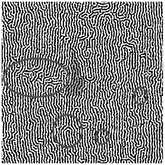
(b)

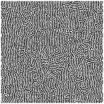
Figure 5: Typical configuration in the nematic-like region at (a) $T=0.114$ and (b) $T=0.116$ for $L=384$. In (a) some defects are put in evidence. In small circles, two pairs of dislocations inside smectic-like domains; in the larger circle a disclination dipole; shown colored a series of dislocations inside a single stripe and in an ellipse a domain of perpendicular orientation.

Analyzing visually the configurations of this region we observe many excitations disrupting orientational order. A typical configuration is shown in Fig. 5. We see that this regime presents large Burgers vector dislocations that can be regarded as a tightly-bound pair of oppositely charged disclinations Toner and Nelson (1981). There are also what may be called a dislocation cascade, a series of bifurcations within a single stripe (colored in Fig. 5a). Small domains of perpendicular orientation (encircled in Fig.(5a)) are present as well, and become more common and larger as temperature increases (see Fig. 5b). Surrounded by topological defects there are domains of locally smectic-like arranged stripes, where order is decorrelated mainly by meandering excitations and all kinds of pairs of dislocations (some are encircled in Fig. 5a).

Figure 6: Orientational correlation length (full symbols) and susceptibility (open symbols) as a function of temperature in the isotropic phase. The continuous curves show power-law fittings, namely: $\xi_{nn}(T)\sim(T-0.1172)^{-1.19}$ and $\chi_{nn}(T)\sim(T-0.1161)^{-0.61}$.

In order to estimate the transition temperature $T_{c}$ between the orientationally ordered and isotropic phases, we have measured the orientational correlation length and susceptibility of $Q$ in the isotropic phase. The results for $L=192$ are shown in Fig. 6 , together with power-law fits. We found that $T_{c}$ lies close to $T_{c}\approx 0.117$ and that divergences are well fitted by power-law forms, at variance with the exponential divergence that one would expect in a defect-mediated transition according to the KTHNY theory Toner and Nelson (1981); Lin et al. (2006). The power law behavior seems to be in agreement with a recent result in which the nematic transition is predicted to be second order Barci and Stariolo .

Finally, we discuss the evolution of the structure factor, eq.(18), with temperature. In Fig. 7 we show four characteristic examples around the transition.

Figure 7: Structure factor at $T=0.1$, $0.114$, $0.118$ and $0.14$ for $L=384$.

From the first to the second plot it can be seen that the sharp peaks characterizing stripe order are replaced by nematic-like peaks, spreaded along the ring $|\mathbf{k}|=k_{m}$ due to angle fluctuations. The transition to the disordered phase seems to be through an increase of domains of perpendicular orientation of the stripes. In the structure factor, this is reflected as the growth of two symmetric peaks around $k\approx k_{m}$ in the perpendicular direction. Immediately after the transition, at $T=0.118$, the four symmetrical peaks are equivalent, as can be seen in the third plot. As the temperature is further increased, angle fluctuations around this two preferential directions smear out the four peaks and the system becomes almost isotropic and the spectral weight of the structure factor lies on a ring with a weakly tetragonal shape, as shown in Fig. 7. A typical configuration illustrating the weakly tetragonal symmetry of the disordered phase just above the transition is shown in Fig. 8.

Not far away from the transition, the isotropic phase still presents the exponential-algebraic behavior of positions correlations as in the nematic-like regime, indicating that it locally resembles the low temperature phase. The anisotropic feature of the orientational correlation function dissapears in this phase, where $C_{nn}$ decays exponentially to zero.

IV Conclusions

We have made Langevin simulations at finite temperature of a model for ultrathin ferromagnetic films with perpendicular anisotropy. These systems have a stripe ground state due to competition between exchange and dipolar interactions. We have found a phase transition from a high temperature disordered phase to a low temperature phase with both translational and orientational orders. Below the transition point isotropy is spontaneously broken, and a smectic-like magnetic structure develops. Both kinds of ordering seem to take place at the same $T_{c}$, in agreement with some previous theoretical predictions. The absence of an intermediate, purely orientational, phase is probably due to the isotropic nature of the model Hamiltonian. Other terms, which explicitly break orientational order, may be necessary in order to have an intermediate nematic phase. This is what emerges from a recent analysis of the nematic transition in this same model, where an extra term was included and shown to be responsible for the existence of an intermediate nematic phase Barci and Stariolo . The nature of these terms depend on microscopic interactions, namely, on the modelling of the anisotropy contribution. In this respect, more input from experiments is fundamental.

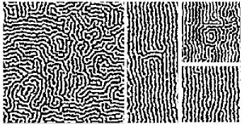
Figure 8: The left configuration shows the isotropic phase at $T=0.12$ for $L=192$, presenting a target defect close to its center. Small target defects are ubiquitous in this phase. At top right we show a large target defect in a portion of a $L=480$ configuration in an out-of-equilibrium disordering process at $T=0.13$. In the middle a portion of a $L=384$ configuration at $T=0.112$ exhibiting a large dislocation pair made of disclination pairs. Below, pairs of dislocations at $T=0.104$.

We have found that the numerical results show complex magnetic structures, with translational and orientational correlations decaying algebraically at low temperatures. Translational correlations have different exponents for the longitudinal and perpendicular components, relative to the ground state stripe orientation. The exponents are also temperature dependent. In the case of orientational correlations, we observe a weak temperature dependence in the perpendicular direction, and a saturation to a constant value in the longitudinal direction. Qualitatively one can say that we observe translational quasi-long-range order and orientational long range order, at low temperatures.

As temperature grows it is possible to observe a proliferation of topological defects, with structures similar to those observed in real systems. In a narrow region around the transition temperature, both translational and orientational corrrelations begin to decay exponentially. A power law fit of the data of the orientational correlation length and the associated susceptibility in the high temperature region allows us to estimate the critical temperature. This power law dependence of the orientational correlation length does not agree with the well known KTHNY theory of two dimensional melting. We do not know to what extent the predictions from this theory should be applicable to magnetic two dimensional systems like this. Our results are in agreement with a possible scenario for a smectic magnetic system put forward by Abanov and coworkers more than 10 years ago Abanov et al. (1995), and with a recent result on the second order nature of the nematic transition in the same model studied in this work supplemented by another term in the Hamiltonian which explicitly breaks orientational order Barci and Stariolo .

We found that the weak anisotropy of the dipolar interaction due to spatial discretization and the short width of the stripes (of three grid points) has led to a pinning effect that favored the stripes orientation to be preferentially on the two Cartesian directions. But looking at the structure factor around the transition, we found that the fluctuations responsible for disrupting orientational order are not restricted to the two Cartesian directions and the isotropic nature of the model still manifests.

More quantitative analytic predictions are clearly needed in order to assess the quality and limitations of our results. Also, it would be extremely interesting to do systematic experimental measurements of structure factors and correlations as a function of temperature, like the ones done by Pescia and coworkers  Vaterlaus et al. (2000); Portmann et al. (2003, 2006). This would allow, between other things, to elucidate the experimental conditions under which a nematic intermediate phase can be present in a magnetic system. The similarity between our simulations and experimental images of perpendicularly magnetized fcc Fe films grown on Cu(100) Vaterlaus et al. (2000); Portmann et al. (2003, 2006) is striking. For example, target defects first observed by Vaterlaus et al. Vaterlaus et al. (2000) were observed in our simulations and are ubiquitous in the disordered phase (see Fig. 8).

Finally, the dynamical behavior of these systems also deserve to be studied, because the presence of frustration and the emergence of many kinds of topological defects lead to a complex dynamics, with pinning of magnetic structures during long time scales, before the final, asymptotic equilibrium state sets in Mulet and Stariolo (2007).

The “Conselho Nacional de Desenvolvimento Científico e Tecnológico CNPq-Brazil” is aknwoledged for financial support. DAS also wants to aknowledge the Abdus Salam International Centre for Theoretical Physics for financial support to the Latinamerican Network on Slow Dynamics in Complex Systems through grant NET-61.

References

- Hubert and Schafer (1998) A. Hubert and R. Schafer, Magnetic Domains (Springer-Verlag, Berlin, 1998).
- Portmann et al. (2003) O. Portmann, A. Vaterlaus, and D. Pescia, Nature 422, 701 (2003).
- Wu et al. (2004) Y. Wu, C. Won, A. Scholl, A. Doran, H. Zhao, X. Jin, and Z. Qiu, Physical Review Letters 93, 117205 (2004).
- Jagla (2004) E. A. Jagla, Phys. Rev. E 70, 046204 (2004).
- Seul and Andelman (1995) M. Seul and D. Andelman, Science 267, 476 (1995).
- Garel and Doniach (1982) T. Garel and S. Doniach, Phys. Rev. B 26, 325 (1982).
- Allenspach et al. (1990) R. Allenspach, M. Stamponi, and A. Bischof, Phys. Rev. Lett. 65, 3344 (1990).
- Politi (1998) P. Politi, Comments Cond. Matter Phys. 18, 191 (1998).
- MacIsaac et al. (1998) A. B. MacIsaac, K. De’Bell, and J. P. Whitehead, Phys. Rev. Lett. 80, 616 (1998).
- Vaterlaus et al. (2000) A. Vaterlaus, C. Stamm, U. Maier, M. G. Pini, P. Politi, and D. Pescia, Phys. Rev. Lett. 84, 2247 (2000).
- Abanov et al. (1995) A. Abanov, V. Kalatsky, V. L. Pokrovsky, and W. M. Saslow, Phys. Rev. B 51, 1023 (1995).
- De’Bell et al. (2000) K. De’Bell, A. B. MacIsaac, and J. P. Whitehead, Rev. Mod. Phys. 72, 225 (2000).
- MacIsaac et al. (1995) A. B. MacIsaac, J. P. Whitehead, M. C. Robinson, and K. De’Bell, Phys. Rev. B 51, 16033 (1995).
- MacIsaac et al. (1996) A. B. MacIsaac, J. P. Whitehead, K. De’Bell, and P. H. Poole, Phys. Rev. Lett. 77, 739 (1996).
- Gleiser et al. (2002) P. M. Gleiser, F. A. Tamarit, and S. A. Cannas, Physica D 168-169, 73 (2002).
- Cannas et al. (2004) S. Cannas, D. Stariolo, and F. Tamarit, Phys. Rev. B 69, 092409 (2004).
- Cannas et al. (2006) S. A. Cannas, M. Michelon, D. A. Stariolo, and F. A. Tamarit, Phys. Rev. B 73, 184425 (2006).
- (18) D. G. Barci and D. A. Stariolo, preprint cond-mat/0611364.
- Mulet and Stariolo (2007) R. Mulet and D. A. Stariolo, Phys. Rev. B 75, 064108 (2007).
- Roland and Desai (1990) C. Roland and R. Desai, Phys. Rev. B 42, 6658 (1990).
- Jagla (2005) E. A. Jagla, Phys. Rev. B 72, 094406 (2005).
- Frenkel and Smith (1996) D. Frenkel and B. Smith, Understanding Molecular Simulation (Academic Press, New York, 1996).
- Vedmedenko et al. (1998) E. Y. Vedmedenko, A. Ghazali, and J. C. S. Lévy, Surface Science 402, 391 (1998).
- Press et al. (1992) W. H. Press, S. A. Teukolsky, W. T. Vetterling, and B. P. Flannery, Numerical Recipes (Cambridge University Press, 1992).
- Frigo and Johnson (2005) M. Frigo and S. G. Johnson, in Proceedings of the IEEE (2005), vol. 93, p. 216.
- Toner and Nelson (1981) J. Toner and D. R. Nelson, Phys. Rev. B 23, 316 (1981).
- Christensen and Bray (1998) J. J. Christensen and A. J. Bray, Phys. Rev. E 58, 5364 (1998).
- Qian and Mazenko (2003) H. Qian and G. F. Mazenko, Phys. Rev. E 67, 036102 (2003).
- Cuesta and Frenkel (1990) J. A. Cuesta and D. Frenkel, Phys. Rev. A 42, 2126 (1990).
- Lin et al. (2006) S. Z. Lin, B. Zheng, and S. Trimper, Phys. Rev. E 73, 066106 (2006).
- Jaster (1999) A. Jaster, Phys. Rev. E 59, 2594 (1999).
- Portmann et al. (2006) O. Portmann, A. Vaterlaus, and D. Pescia, Phys. Rev. Lett. 96, 047212 (2006).