Quantum chaos in the mesoscopic device for the Josephson flux qubit

Abstract

We study the quantum spectra and eigenfunctions of the three-junction SQUID device designed for the Josephson flux qubit at high energies. We analyze the spectral statistics on the parameter region where the system has a mixed classical phase space where regular and chaotic orbits can be found at the same classical energy. We perform a numerical calculation of eigenvalues and eigenstates for different values of the ratio of the Josephson and charging energies, $E_{J}/E_{C}$, which is directly related to an effective $\hbar$ parameter. We find that the nearest neighbour distributions $P(s)$ of the energy level spacings are well fitted by the Berry-Robnik theory employing as free parameters the pure classical measures of the chaotic and regular regions of phase space in the different energy regions in the semiclassical case. The phase space representation of the wave functions is obtained via the Husimi distributions and the localization of the states on classical structures is analyzed. We discuss for which values of $E_{J}/E_{C}$ it can be possible to perform experiments that could be sensitive to the structure of a mixed classical phase space.

I Introduction

In recent years, several types of superconducting qubits have been experimentally proposed.nakamura ; qbit_mooij ; vion ; martinis These systems consist on mesoscopic Josephson devices and they are promising candidates to be used for the design of qubits for quantum computation.nakamura ; qbit_mooij ; vion ; martinis ; revqubits ; chiorescu ; fqubit_recent Indeed, a large effort is devoted to succeed in the coherent manipulation of their quantum states in a controlable way. The progress made in this case allows to have nowadays Josephson circuits with small dissipation and large decoherence times.vion ; martinis ; chiorescu ; fqubit_recent Very recently, it has been proposed that, due to these developments, it could also be possible to use mesoscopic Josephson devices for the study of the quantum signatures of classically chaotic systems.montangero05 ; mingo In Ref. mingo, the quantum dynamics of the Device for the Josephson Flux Qubit (DJFQ) has been studied. In particular, it has been discussed how the fidelity (or Loschmidt echo)jp of the DJFQ could be studied experimentally for energies corresponding to the hard chaos regime in the classical limit. Here, we extend the work of Ref. mingo, by analyzing the possibility of studying, in the DJFQ, the mixed chaos regime (i.e., the energy range where there is a coexistence of chaotic and regular orbits in the classical limit). To this end, standard tools of analysis of “quantum chaos”, like spectral statistics metha ; bohigas ; berryro ; seligman ; cederbaum84 ; cederbaum86 ; prosen ; makino01 ; robnik05 and phase space distributions,wigner ; husimi ; hus-rev ; groh will be used.

It is by now well established that from the analysis of the spectral properties of quantum systems in the semiclassical regime it is possible to obtain information about the underlying dynamics of the classical counterpart. metha ; bohigas ; berryro ; seligman ; cederbaum84 ; cederbaum86 ; prosen ; makino01 ; robnik05 The probability distribution $P(s)$ of the spacings $s$ between successive energy levels - the nearest neighbor spacing distribution $P(s)$- unveils information on the associated classical dynamics. For integrable systems the levels are uncorrelated, and $P(s)$ obeys a Poisson distribution. For completely chaotic classical motion, $P(s)$ follows the prediction of the Random Matrix Theory (RMT) metha and when time reversal symmetry is preserved $P(s)$ is closely approximated by the Wigner distribution for the Gaussian Orthogonal Ensemble (GOE), $P(s)\sim s\exp{(-s^{2})}$.bohigas

Generic quantum systems do not conform to the above special cases, the classical phase space typically presents mixed dynamics, with coexistence of regular orbits and chaotic motion.berryro ; seligman ; cederbaum84 ; cederbaum86 ; prosen ; makino01 ; robnik05 In this generic case Berry and Robnik berryro proposed an analytical expression for the corresponding $P(s)$, based on the knowledge of pure classical quantities related to the Liouville measure of the chaotic and regular classical regions. The idea behind their calculations is that each regular or irregular phase space region gives rise to its own sequence of energy levels. For each region the level density results proportional to the Liouville measure of the classical region and the associated level spacing distribution follows the Poisson or the Wigner form for regular and chaotic regions respectively. In the semiclassical limit these sequences of energy levels can be supposed independent and the complete distribution $P(s)$ is obtained by their random superposition. Several works have studied numerically the level statistics in systems with mixed dynamics. seligman ; cederbaum84 ; cederbaum86 ; prosen ; makino01 ; robnik05 Systems with two degrees of freedom have been analyzed by several groups, mostly quartic oscillatorsseligman ; cederbaum84 ; cederbaum86 and billiards,prosen ; makino01 ; robnik05 and in some works the Berry-Robnik proposal has been tested in detail.cederbaum86 ; prosen ; makino01

In contrast to the level statistics, the wave functions of quantum chaotic systems have remained relatively less explored. In particular the analysis of wave functions in phase space representations, such as the Wigner function wigner or the Husimi distribution, husimi ; hus-rev ; groh allows a direct comparison between the classical and the quantum dynamics. Of particular interest are the zeros of the Husimi distribution which seem to be organized along regular lines or fill space regions for regular or chaotic classical dynamics respectively. leboeuf

Besides the importance of visualizing the dynamical properties of quantum systems in phase space, techniques for measuring these functions, referred as “quantum tomography ” nielsen ; miquel are subjects of active research in many experimental systems, like ion traps, optical lattices, entangled photons,mitchell ; kanem and also superconducting qubits.tomo_super

Josephson junctions have been used for the study of classical chaos since the early 1980s.jchaos ; jchaos_exp A single underdamped junction with a periodic current drive can become chaotic in a wide range of parameter values.jchaos Several experiments have indeed studied this problem and measured chaotic properties in current-voltage curves and in voltage noise in Josephson junctions.jchaos_exp Moreover, networks with several junctions have been proposed for the study of spatio-temporal chaos.jchaos_arrays All this cases correspond to classical chaos in dissipative systems with a time-periodic drive. Much less studied has been the case of classical hamiltonian chaos in Josephson junctions,parmenter mainly due to the fact that dissipation through a shunt resistance and/or coupling to the external measuring circuitry is typically important. For the same reason, i.e., the difficulty in fabricating Josephson circuits with negligible coupling to the environment, few examples of quantum chaos in Josephson systems are found in the literature. One of them is the work of Graham et al.,graham who considered dynamical localization and level repulsion in a single Josephson junction with a time periodic drive. More recently T. D. Clark, M. J. Everitt and coworkerseveritt explored chaos and the quantum behaviour of SQUID rings coupled to electromagnetic field modes. The recent development of Josephson devices for quantum computation, which need large coherence times, lead to significant advances in the fabrication of circuits with small coupling to the external circuit and negligible dissipation. This opened the possibility of using this type of mesoscopic devices for the study of quantum chaos. For example, Montangero et al. montangero05 have proposed recently a Josephson nanocircuit as a realization of the quantum kicked rotator. The difficulty in realizing experimentally their system resides in that it needs to move mechanically one superconducting node in a high-frequency periodic motion. A different proposal has been put forward in Ref.mingo, , where it has been shown that the Device for the Josephson Flux Qubit (DJFQ),qbit_mooij ; chiorescu ; fqubit_recent which consists on a three-junction SQUID, is classically chaotic at high energies. It could be therefore possible to use this system for the experimental study of quantum signatures of classical chaos. One possibility is the analysis of the fidelity or Loschmidt echojp in the quantum dynamics.mingo An experimental setup for the measurement of the Loschmidt echo in the DJFQ has been proposed in Ref.mingo, . In the above mentioned work, the system is prepared initially with a wave packetnota2 localized in coordinate (phase) and momentum (charge) with an energy corresponding to the regime of hard chaos in the classical limit. The quantum evolution of the wave packet is evaluated in the unperturbed and the perturbed hamiltonians, and the overlap of the two evolved wave functions defines the Loschmidt echo or fidelityjp , which can be measured experimentally.mingo Different behavior could be observed if the wave packet is initially localized in a chaotic or in a regular region of the phase space. Therefore, an interesting case to analyze is when the wave packet is prepared initially with an energy within the regime where there is a mixed phase space in the classical limit. In this case, one would expect that the behavior of the Loschmidt echo could depend on the location of the average coordinate and momentum of the initial wave packet. For example, in Ref.liu, it has been found a strong dependence of the fidelity with the initial state for mixed dynamics in the phase space in the case of Bose-Einstein condensates. However, in order to be sensitive to the structure of phase space in the case of mixed dynamics, it is necessary to have a small effective $\hbar$. The aim of the present work is to analyze the quantum spectra and wave functions of the DJFQ in order to obtain for which values of the effective $\hbar$ the quantum physics of this system can show signatures of the structure of the phase space in the case of mixed dynamics. To this end, we will use standard tools of quantum chaos theory by calculating numerically the level statistics of the DJFQ for different effective $\hbar$ and the Husimi distribution.

Concerning the spectral analysis, the quantum signatures of chaos have been discussed through the $P(s)$ distribution in Ref. kato, for a SQUID with three junctions in the hard chaos regime. However, the case with only on-site capacitances was considered there (the capacitance of the junctions was neglected). Nevertheless, the device for the Josephson flux qubit fabricated by the Delft goupchiorescu has small on-site capacitances, about two orders of magnitude smaller than the intrinsic capacitances of the junctions.nota3 This fact turns the model hamiltonian for the DJFQ to be different from the one studied in Refs.parmenter, ; kato, . One of the goals of this paper is to analyze the spectral properties of the DJFQ considering realistic values of the different capacitances to analyze the device for the Josephson flux qubit (DJFQ) in the case of mixed dynamics. In addition we analyze the structure of the Husimi functions for the DJFQ, an issue that has been so far unexplored. The paper is organized as follows. In Sec.II we introduce the quantum model for the device for the Josephson flux qubit. Before presenting the quantum spectral analysis, we will study in Sec. III the dynamics of its classical analog. The presence of chaos will be characterized through the analysis of a measure of the chaotic volume, that will be defined and obtained as a function of the energy. We devote the rest of Sec. III to the analysis of the spectral properties. The NNS distribution will be obtained for different energies corresponding to different classical energy regions and dynamics and for different values of the effective $\hbar$. In Sec. IV we compute the Husimi distribution for the DJFQ in order to characterize the localization of the quantum states on typical phase space structures related to the different classical regimes. Finally in Sec. V we summarize our results and discuss possible experimental characterizations of the quantum manifestations of chaos in this system.

II Model for the Device for the Josephson Flux Qubit

The DJFQ consists of three Josephson junctions in a superconducting ring qbit_mooij that encloses a magnetic flux $\Phi=f\Phi_{0}$, with $\Phi_{0}=h/2e$, see Fig.1.

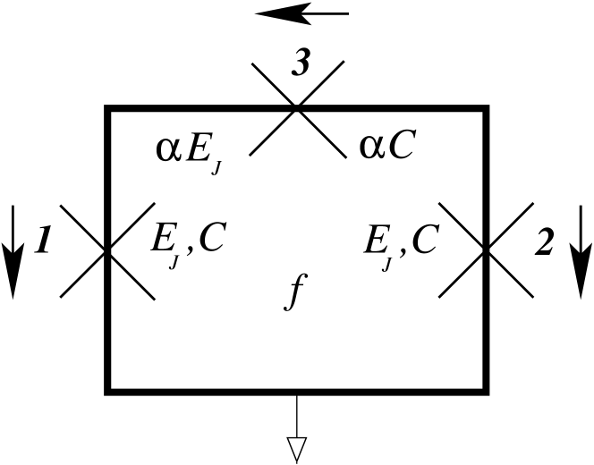
Figure 1: Circuit for the Device for the Josepshon Flux Qubit as described in the text. Josepshon junctions $1$ and $2$ have Josepshon energy $E_{J}$ and capacitance $C$, and junction $3$ has Josepshon energy and capacitance $\alpha$ times smaller. The arrows indicate the sign convention for defining the gauge invariant phase differences. The circuit encloses a magnetic flux $\Phi=f\Phi_{0}$.

The junctions have gauge invariant phase differences defined as $\varphi_{1}$, $\varphi_{2}$ and $\varphi_{3}$, respectivily, with the sign convention corresponding to the directions indicated by the arrows in Fig.1. Typically the circuit inductance can be neglected and the phase difference of the third junction is: $\varphi_{3}=-\varphi_{1}+\varphi_{2}-2\pi f$. Therefore the system can be described with two dynamical variables: $\varphi_{1},\varphi_{2}$. The circuits that are used for the Josephson flux qubit have two of the junctions with the same coupling energy, $E_{J,1}=E_{J,2}=E_{J}$, and capacitance, $C_{1}=C_{2}=C$, while the third junction has smaller coupling $E_{J,3}=\alpha E_{J}$ and capacitance $C_{3}=\alpha C$, with $0.5<\alpha<1$. The above considerations lead to the Hamiltonian qbit_mooij ; nota

$${\cal H}=\frac{1}{2}{\vec{P}}^{T}{\rm{\bf M}}^{-1}{\vec{P}}+E_{J}V(\vec{\bf\varphi})$$ (1)

where the two-dimensional coordinate is $\vec{\varphi}=(\varphi_{1},\varphi_{2})$. The potential energy is given by the Josephson energy of the circuit and, in units of $E_{J}$, is:

$$V(\vec{\bf\varphi})=2+\alpha-\cos\varphi_{1}-\cos\varphi_{2}-\alpha\cos(2\pi f+\varphi_{1}-\varphi_{2})\;.$$ (2)

The kinetic energy term is given by the electrostatic energy of the circuit, where the two-dimensional momentum is

$$\vec{P}=(P_{1},P_{2})={\rm{\bf M}}\cdot\frac{d{\vec{\varphi}}}{dt},$$

and $\bf M$ is an effective mass tensor determined by the capacitances of the circuit,

$${\rm{\bf M}}=C{\left(\frac{\Phi_{0}}{2\pi}\right)^{2}}{\rm{\bf m}}$$

with

$${\rm{\bf m}}=\left({{\begin{array}[]{cc}{1+\alpha+\gamma}&{-\alpha}\\ {-\alpha}&{1+\alpha+\gamma}\\ \end{array}}}\right).$$

We included in $\bf M$ the on-site capacitance $C_{g}=\gamma C$. (Typically $\gamma\sim 10^{-2}-10^{-3}\ll 1$). In the presence of gate charges $Q_{g,i}$ induced in the islands, the momentum is ${\vec{P}}\rightarrow{\vec{P}}+\frac{\Phi_{0}}{2\pi}\vec{Q_{g}}$.qbit_mooij The system modelled with Eqs. (1)-(2) is analogous to a particle with anysotropic mass ${\rm{\bf M}}$ in a two-dimensional periodic potential $V(\vec{\bf\varphi})$.geisel

In typical junctions, the Josephson energy scale, $E_{J}$, is much larger than the electrostatic energy of electrons, $E_{C}=e^{2}/2C$, and the system is in a classical regime. On the other hand, mesoscopic junctions (with small area) can have $E_{J}\sim E_{C}$, and quantum fluctuations become important.likharev In this case, the quantum momentum operator is defined as

$${\vec{P}}\rightarrow\hat{\vec{P}}=-i\hbar\nabla_{\varphi}=-i\hbar(\frac{\partial}{\partial\varphi_{1}},\frac{\partial}{\partial\varphi_{2}}).$$

After replacing the above defined operator $\hat{\vec{P}}$ in the Hamiltonian of Eq.(1), the eigenvalue Schrödinger equation becomes

$$\left[-\frac{\eta^{2}}{2}\nabla_{\varphi}^{T}{\rm{\bf m}}^{-1}\nabla_{\varphi}+V(\vec{\bf\varphi})\right]\Psi(\vec{\bf\varphi})=E\Psi(\vec{\bf\varphi})\;,$$ (3)

where we normalized energy by $E_{J}$ and momentum by $\hbar/\sqrt{8E_{C}/E_{J}}$. We see in Eq.(3) that the parameter $\eta=\sqrt{8E_{C}/E_{J}}$ plays the role of an effective $\hbar$. It is well-known that the ratio $E_{C}/E_{J}$ controls the effect of quantum fluctuations in single Josephson junctionsschon ; haviland and in arrays of several Josephson junctions.fazio ; mooij_qjja For $E_{J}\gg E_{C}$, ($\eta\ll 1$), the junctions can be described with a classical dynamics; while for $E_{J}\sim E_{C}$, ($\eta\sim 1$) the effect of quantum fluctuations becomes important.schon Experiments where the Josephson junctions are fabricated for different values of $E_{C}/E_{J}$ have been performed both for single junctionshaviland and for junction arrays.mooij_qjja In the last case quantum phase transitions as a function of $E_{C}/E_{J}$ have been studied.fazio ; mooij_qjja Therefore, the parameter $\eta=\sqrt{8E_{C}/E_{J}}$ is a natural choice for quantifying the effective $\hbar$ in this system.

For quantum computation implementations qbit_mooij ; chiorescu ; fqubit_recent the DJFQ is operated at magnetic fields near the half-flux quantum ($f=f_{0}+\delta f$, with $f_{0}=1/2$). For values of $\alpha\geq 1/2$, the potential Eq.(2) has two well defined minima. At the optimal operation point $f=1/2$, the two lowest (degenerated) energy states are symmetric and antisymmetric superpositions of two states corresponding to macroscopic persistent currents of opposite sign. The offset value $\delta f$ determines the level splitting between these two states. These eigenstates are energetically separated from the others (for small $\delta f$) and therefore the DJFQ has been used as a qubit qbit_mooij ; chiorescu ; fqubit_recent (i.e. a two-level truncation of the Hilbert space is performed). In addition the barrier for quantum tunneling between the states depends strongly on value of $\alpha$ and its height goes up as $\alpha$ is increased. The possibility to manipulate the potential landscape by changing $\alpha$ is a crucial point for experimental implementation of qubits. Typical experiments in DJFQ have values of $\alpha$ in the range $0.6-0.8$.chiorescu ; fqubit_recent

As we will discuss here, the higher energy states of the DJFQ show quantum manifestations of classical chaos. In what follows we focus our study of the DJFQ considering the realistic case of: (i) small on-site capacitances, taking $\gamma=0.02$, (ii) a magnetic field corresponding to the optimal operation point of the DJFQ, $f=1/2$, and (iii) the values of $\alpha=0.7$ and $0.8$ in coincidence with the experimental values employed in Ref. chiorescu, ; fqubit_recent, .

III Spectral Statistics

Before entering into the analysis of the quantum spectra we will focus on the classical dynamics of the DJFQ. As we already anticipated in the Introduction, generic systems present mixed classical dynamics and the DJFQ is not the exception. Therefore for a given energy $E$ our aim is to estimate the chaotic volume $v_{\rm ch}(E)$, defined as the probability of having a chaotic orbit (i.e. Lyapunov exponent $\lambda>0$) at energy $E$. As we will show below, this parameter will be relevant in the statistical analysis of the quantum spectrum.

The classical dynamical evolution was obtained solving the Hamilton equations derived from Eq.(1):

$${\rm{\bf m}}\cdot\frac{d^{2}{\vec{\varphi}}}{dt^{2}}=-\nabla_{\varphi}V(\vec{\bf\varphi}),$$ (4)

where we have normalized energy by $E_{J}$ and time by $t_{c}=\sqrt{\hbar^{2}C/4e^{2}E_{J}}=\hbar/\eta E_{J}$ (the Josephson plasma frequency is $\omega_{p}=t_{c}^{-1}$). The numerical integration was performed with a second-order leap-frog algorithm with time step $\Delta t=0.02t_{c}$.

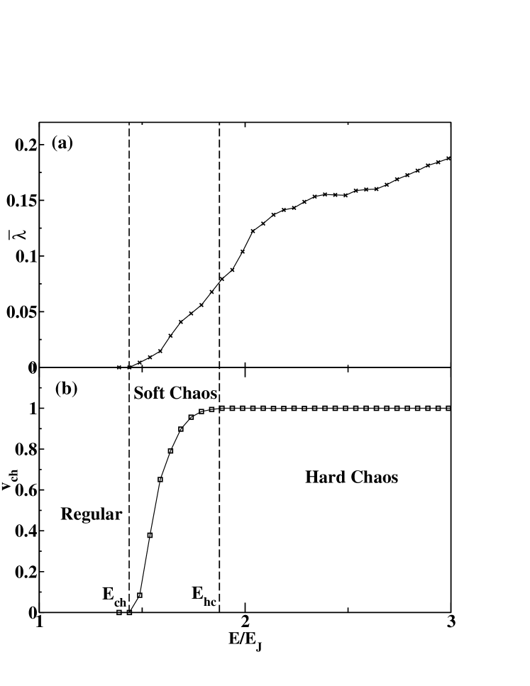
Figure 2: (a) Average maximum Lyapunov exponent $\overline{\lambda}$ and (b) chaotic volume $v_{ch}$ versus energy $E$ for $\alpha=0.8$ and $f=1/2$.

For different values of the parameter $\alpha$ and magnetic flux $f$ we compute the maximum Lyapunov exponent $\lambda$ for each classical orbit at different energies $E$. We estimate the chaotic volume $v_{\rm ch}(E)$ using $10^{3}$ initial conditions chosen randomly with uniform probability within the available phase space for each given energy. Also the average Lyapunov exponent, $\bar{\lambda}(E)$, of the chaotic orbits is obtained. These results are shown in Fig. 2 for $\alpha=0.8$ and $f=1/2$. We observe that both $v_{\rm ch}(E)$ and $\bar{\lambda}(E)$ increase smoothly with energy, as it is usual in several similar systems with two degrees of freedom.benettin ; meyer ; cejnar Above the minimum energy of the potential, $E_{min}$, we find: (i) regular orbits for $E_{min}<E<E_{ch}$ ($v_{\rm ch}=0$), (ii) soft chaos (i.e., coexistence of regular and chaotic orbits, $0<v_{\rm ch}<1$) for $E_{ch}<E<E_{hc}$ with the average Lyapunov exponent $\bar{\lambda}>0$ above $E_{ch}$ and (iii) hard chaos (all orbits are chaotic, $v_{\rm ch}=1$) for $E>E_{ch}$. The boundaries of these different dynamic regimes as a function of $\alpha$, in the range $[0.5,1.0]$, and $f$, in the range $[0,0.5]$, have been obtained in Ref. mingo, . Here we will focus on the case with $f=1/2$ and we will study some different cases of $\alpha$.

In order to look for signatures of quantum chaos, we follow a standard statistical analysis of the energy spectrum. First we calculate the exact spectrum $\{E_{n}\}$ by diagonalization of the quantum Hamiltonian. The eigenvalue equation Eq.(3) is solved by discretizing the phases with $\Delta\varphi=2\pi/1000$, and the resulting hamiltonian matrices of size $10^{6}\times 10^{6}$ are diagonalized using standard algorithms for sparse matrices. We have verified that increasing the discretization by a factor of $2$ does not affect the results of the spectrum within the needed accuracy for the ranges of energies studied here. As we mentioned we set $\gamma=0.02$ and $f=1/2$, and we obtain eigenvalue spectra for different values of the parameters $\eta$ and $\alpha$ defined in the previous section.

The level spectrum is used to obtain the smoothed counting function $N_{av}(E)$ which gives the cumulative number of states below an energy $E$. In order to analize the structure of the level fluctuations properties one unfolds the spectrum by applying the well kwown transformation $x_{n}=N_{av}(E_{n})$.bohigas From the unfolded spectrum one can calculate the nearest-neighbor spacing (NNS) distribution $P(s)$, where $s_{i}\equiv x_{i+1}-x_{i}$ is the NNS.

We have taken into account the symmetries of the Hamiltonian Eq.(1). For $f=1/2$ the Hamiltonian has reflection symmetry against the axis $\varphi_{2}=\varphi_{1}$ and against the axis $\varphi_{2}=-\varphi_{1}$. The eigenstates can be chosen with a given parity with respect to these two symmetry lines. Therefore, we compute the NNS distribution employing eigenstates of a given parity. This kind of decomposition is a standard procedure followed in the analysis of spectral properties of quantum systems whenever the Hamiltonian of the system possesses a discrete symmetry.bohigas We consider the even-even parity states and the NNS distribution is computed for different energy regions inside the classical interval ($E_{ch},E_{hc}$), corresponding to soft chaos, and for energies $E>E_{hc}$ ( and $E<2\Delta$), corresponding to hard chaos.

The Berry- Robnik theory seems to be suitable to analyze, in the semiclassical regime, sequence of levels of quantum systems whose classical analogous presents coexistency of regular and chaotic dynamics (i.e., soft chaos regime). If $\rho_{1}$ and $\rho_{2}$ are the relative measures of the regular and chaotic parts of the classical phase space then, the Berry-Robnik distribution berryro reads:

$$P^{BR}(s)=\rho_{1}^{2}\exp{(-\rho_{1}s)}\;\mbox{erfc}\left(\frac{1}{2}\sqrt{\pi}\rho_{2}s\right)+$$

$$\left(2\rho_{1}\rho_{2}+\frac{1}{2}\pi\rho_{2}^{3}s\right)\exp\left(-\rho_{1}s-\frac{1}{4}\pi\rho_{2}^{2}s^{2}\right)\;,$$ (5)

where $\rho_{1}+\rho_{2}=1$. It is easy to verify that $P^{BR}(s)$ interpolates between the Poisson and Wigner GOE distributions as $0\rightarrow\rho_{1}\rightarrow 1$, but does not exhibit level repulsion for $\rho_{1}\neq 0$.

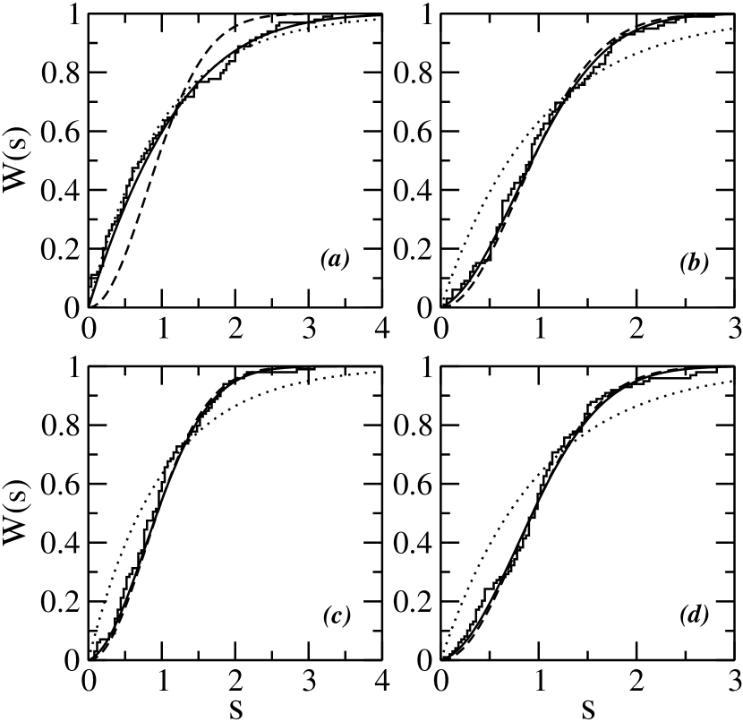
Figure 3: Cumulative distribution $W(s)$ for $\alpha=0.8$ and $f=0.5$. See the text for details. The continuous line is the fitted Berry-Robnik distribution. We show for comparison the Poisson (dotted line) and Wigner (dashed line) cumulative distributions. Top panels correspond to $E=1.6$ with (a) $\eta=0.01$ and (b) $\eta=0.05$. Bottom panels correspond to $E=2.0$ with (c) $\eta=0.01$ and (d) $\eta=0.05$. The fitted Berry-Robnik parameters are (a) $\rho_{br}=0.44$, (b) $\rho_{br}=0.93$, (c) $\rho_{br}=0.99$ and (d) $\rho_{br}=0.96$.

In Fig.3 we show the cumulative level spacing distribution $W(s)=\int P(s)ds$ obtained numerically following the prescription described before. We have done this in order to describe in some detail the behavior for small values of $s$, (in the following we denote the cumulative distributions by the same name that the corresponding NNS distribution). In all the cases we have fitted the numerically obtained $W(s)$ employing Eq.(III) for the NNS distribution, and we have extracted the fitted quantum parameter $\rho_{1}\equiv\rho_{br}$.

The particular results presented in Fig. 3 correspond to a window of $\sim 100$ eigenvalues around $E_{ch}<E=1.6<E_{hc}$, within the soft chaos regime, Fig. 3 (a),(b); and $E_{hc}<E=2$, within the hard chaos regime, Fig. 3 (c),(d). We take the realistic experimental value for the parameter $\alpha=0.8$ and consider different values of the quantum parameter $\eta$ : the case with $\eta=0.01$ is shown in Fig. 3 (a),(c); and the case with $\eta=0.05$ is shown in Fig. 3 (b),(d). We should remark that the classical dynamics is independent of the parameter $\eta$, which has a pure quantum origin and plays the role of an effective Planck’s constant in the Schrödinger equation, as we mentioned before. In addition in Fig.3 we show for comparison the $W(s)$ corresponding to the Poisson and Wigner GOE distributions.

We first discuss the case with $\eta=0.05$, that is already smaller than in the cases studied in Ref.mingo, , where $\eta=0.07-0.17$ was considered. The numerical results for $\eta=0.05$, in the case of hard chaos [$E=2.0$, shown in Fig. 3 (d)], are in good agreement with the Wigner distribution, and we obtain $\rho_{br}=0.96$. In a case corresponding to mixed classical dynamics [$E=1.6$, shown in Fig. 3 (b)], we find that the distribution departs slightly from the pure Wigner form. However, we have obtained $\rho_{br}=0.93\gg v_{ch}\sim 0.4$, meaning that the level distribution in this case does not seem to be very sensitive to the mixed phase space expected in the classical limit. The reason is that for increasing $\eta$ the mean energy level spacing increases (proportional to $\eta^{2}$ for large energies), and therefore the width of the energy region evaluated for the statistics with a given number of levels ($\sim 100$ in this case) also increases in the same way. Since $v_{ch}(E)$ varies rapidly with $E$ within the soft chaos region, relating its value with the fitted $\rho_{br}$, which is obtained evaluating the statistics over a wide energy region, becomes meaningless for large $\eta$. Indeed, deep in the quantum regime the Berry-Robnik fitted parameters are not expected to be related to the classical measure of the chaotic (regular) part of the phase space.berryro ; cederbaum86 ; prosen

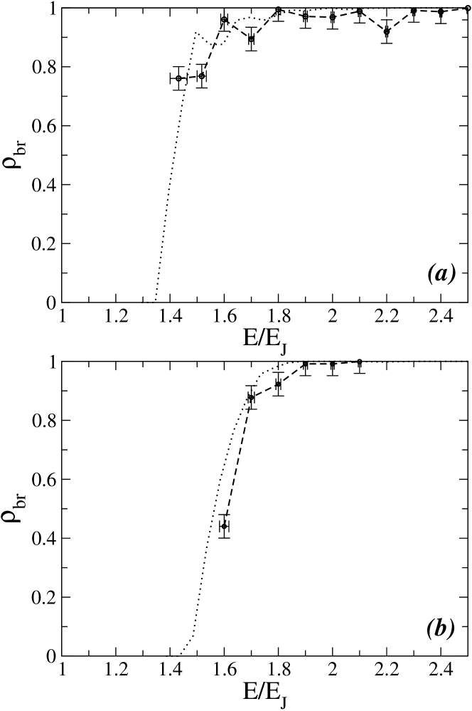
Figure 4: Fitted Berry-Robnik parameter $\rho_{br}$ as a function of the dimensionless energy $E/E_{J}$ for $f=0.5$ and $\eta=0.01$. (a) $\alpha=0.7$ and (b) $\alpha=0.8$. The horizontal error bars in energy are defined by the interval of eigenenergies used in the statistics, and it is a decreasing function of the density of states. The vertical error bars correspond to error in the parameter $\rho_{br}$ as obtained from the numerical fits. The dotted line shows the chaotic fraction of the classical phase space $v_{ch}$ obtained from the classical dynamics.

We now discuss a smaller value of the effective $\hbar$, corresponding to $\eta=0.01$. In Fig.  3 (a), for $E=1.6$ (mixed classical dynamics), we find now that the $W(s)$ clearly departs from the pure Wigner form, and that it can be fitted with the Berry- Robnik distribution with $\rho_{br}=0.44$. This value is very close to the classical chaotic volume for this case, $v_{ch}\approx 0.4$. In the case for $E=2$ (hard chaos), shown in Fig.3 (c), we have obtained $\rho_{br}=0.99$, in agreement with $v_{ch}=1$ and also in good agreement with the Wigner distribution, as expected.bohigas ; seligman

In general we find that in a nearly semiclassical regime, $\eta=0.01$, the numerical results for the Berry-Robnik parameter $\rho_{br}$ show a good agreement with the classical measure $\rho_{1}$, that by definition is equivalent to the chaotic volume $v_{ch}$. This is analyzed in Fig. 4 where we plot the quantum parameter $\rho_{br}$ obtained for different sections of the spectra with $\sim 100$ eigenvalues around a given energy $E$. We show results for two cases of the parameter $\alpha$. The chaotic fraction of the classical phase space $v_{ch}$ is also plotted. The results for $\rho_{br}$ and $v_{ch}$ are very close to each other. When changing the parameter $\alpha$ the location in energy of the onsets of the soft chaos and hard chaos regimes shifts. We also see that the curves of $\rho_{br}$ vs. $E$ shift in the same way, giving further support to the correspondence between $\rho_{br}$ and $v_{ch}$.seligman ; cederbaum86 ; prosen ; makino01 These results corroborate the validity of the Berry-Robnik theory in the semiclassical energy region that corresponds to small effective Planck’s constant, as it is the case for $\eta=0.01$.

Besides the cases reported above, we have also analyzed a few other values of $\alpha$ in the range $0.5-0.9$ and $f=0.4,0.5$, obtaining similar results for the spectral statistics. In general, we observe that in order to obtain a spectral statistics with a Berry-Robnik paremeter that agrees with the classical measure of the chaotic volume values of $\eta<0.05$ are needed.

IV Phase space and Husimi Distributions for the DJFQ

In this section we pursue our study of the signatures of quantum chaos presenting an analysis of the quantum phase-space distributions in the case of mixed classical dynamics. Taking into account the analysis of the previous section we focus on the case $\eta=0.01$.

Quantum phase space distributions are of increasing interest in studies of quantum chaos because they allow a direct comparison between classical and quantum dynamics. The Husimi distribution associated to a quantum wave function $|\Psi\rangle$ (see definition below, Eq.( 6)) it is based on the coherent-state representation and is well suited to represent wave functions in phase space because it is always real and possitive.husimi ; leboeuf ; hus-rev ; groh Due to these properties it is usually referred as a quasi probability distribution.

In order to compute the Husimi function for the DJFQ we must take into account the fact that the classical phase space is four dimensional. The Husimi distribution function for a state $|\Psi\rangle$ is

$$\rho^{H}(\vec{P_{0}},\vec{\varphi_{0}})=|\langle\vec{P_{0}},\vec{\varphi_{0}}|\Psi\rangle|^{2}\;,$$ (6)

where $|\vec{P_{0}},\vec{\varphi_{0}}\rangle$ corresponds to minimum-uncertainty $2\pi$-periodical wave packets carruthers given by

$$|\vec{P_{0}},\vec{\varphi_{0}}\rangle = C\times\exp[i\vec{K_{0}}\cdot\left(\vec{\varphi}-\vec{\varphi_{0}}\right)]\times$$

$$\exp\left[\frac{\cos(\varphi_{0,1}-\varphi_{1})+\cos(\varphi_{0,2}-\varphi_{2})-2}{2\sigma^{2}}\right]$$

where $\vec{K_{0}}=(k_{1},k_{2})$ with $k_{1},k_{2}$ integers and $\vec{P_{0}}=\eta\vec{K_{0}}$. The width of the wave packet is $\sigma=\sqrt{\eta/s}$, with $s$ the squeezing parameter, and we choose the value $s=3.23$, which is the same value used in Ref.mingo, for the initial coherent wave packets.

The potential has two minima for $f=1/2$ which are at $(\varphi^{*},-\varphi^{*})$ and $(-\varphi^{*},\varphi^{*})$, with $\cos\varphi^{*}=1/2\alpha$. To better analyze the Husimi function, it is convenient to make the following change of variables:

$$\varphi_{x} = \frac{\varphi_{1}-\varphi_{2}}{\sqrt{2}},\;\;\;\;\;\;\;P_{x}=\frac{P_{1}-P_{2}}{\sqrt{2}};$$

$$\varphi_{y} = \frac{\varphi_{1}+\varphi_{2}}{\sqrt{2}},\;\;\;\;\;\;\;P_{y}=\frac{P_{1}+P_{2}}{\sqrt{2}}.$$ (8)

In this way the two minima lie along the direction of $\varphi_{x}$. The normalization by $\sqrt{2}$ is chosen such that new variables satisfy $[\varphi_{x},P_{x}]=i\eta$, $[\varphi_{y},P_{y}]=i\eta$ in the quantum regime.

The classical Poincaré surface of section is calculated in the plane $(\varphi_{x},P_{x})$, taking $\varphi_{y}=0$ and $P_{y}>0$. We want to compare the Husimi distribution $\rho^{H}_{\nu}(\vec{K},\vec{\varphi})$ corresponding to the eigenstate $|\Psi_{\nu}\rangle$ with eigenvalue $E_{\nu}$ with the classical Poincaré section at an energy $E\approx E_{\nu}$. To this end, we construct an analog of the surface of section by obtaining a two-dimensional section of $\rho^{H}_{\nu}(\vec{K},\vec{\varphi})$ (which is a four-dimensional density in phase space) in the following way:groh

$$\Phi^{H}_{\nu}(P_{x},\varphi_{x})=\rho_{\nu}^{H}(P_{x},P_{y}^{E};\varphi_{x},0)$$ (9)

where, given the values $P_{x},\varphi_{x}$ and $\varphi_{y}=0$, $P_{y}^{E}$ is obtained such that the classical energy is equal to $E$ and the possitive root, $P_{y}^{E}>0$, is chosen.

We obtain numerically the eigenstates $|\Psi_{\nu}\rangle$ of Eq. (3), after using a discretization of $\Delta\varphi=2\pi/500$. Then, using Eqs. (6)-(9), we compute the sections of the Husimi distributions, $\Phi^{H}_{\nu}(P_{x},\varphi_{x})$. In order to characterize the localization of the quantum states on the classical phase space structures, we choose a few examples of $\Phi^{H}_{\nu}$ for eigenstates that lie in energy regions corresponding to regular classical dynamics $E<E_{ch}$ and soft chaos region, $E_{ch}<E<E_{hc}$, respectively.

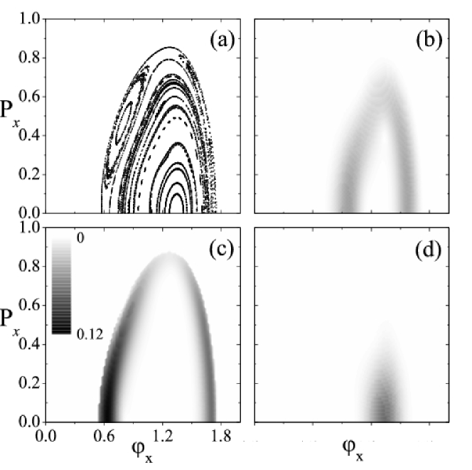
Figure 5: (a) Classical Poincaré surface of section for $E=1.52$. Sections are symmetric with respect to $\varphi_{x}\rightarrow-\varphi_{x}$ and $P_{x}\rightarrow-P_{x}$; only the region of $\varphi_{x}>0$ and $P_{x}>0$ is shown. Section of Husimi phase space distribution, $\Phi^{H}_{\nu}(P_{x},\varphi_{x})$ for (b) $E_{\nu}=1.5219$, (c) $E_{\nu}=1.5208$, (d) $E_{\nu}=1.5193$.

In Fig. 5 (a) we plot for $E=1.52<E_{ch}$ the classical Poincaré section in which the stability islands associated to the regular dynamics are observed. We have computed the Husimi phase space distributions $\Phi^{H}_{\nu}(P_{x},\varphi_{x})$ for several eigenstates ($\sim 20$) near the energy $E=1.52$. We show here three cases corresponding to eigenstates with energies $E_{\nu}=1.5219$, $E_{\nu}=1.5208$ and $E_{\nu}=1.5193$ (panels (a) , (b) and (c) respectively). The localization of these states on the stability islands and fixed points is clearly observed.

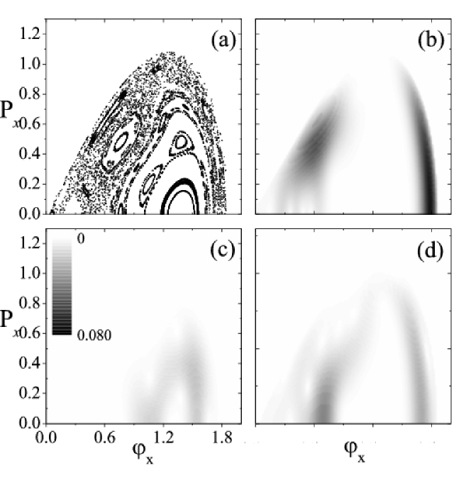
Figure 6: Classical Poincaré surface of section for $E=1.6$. Section of Husimi phase space distribution, $\Phi^{H}_{\nu}(P_{x},\varphi_{x})$ for (b) $E_{\nu}=1.601$, (c) $E_{\nu}=1.6008$, (d) $E_{\nu}=1.5993$.

In Fig.6(a) and Fig.7(a) we plot for classical energies $E=1.6$ and $E=1.7$ respectively, the classical Poincaré sections together with a selection of some of the calculated Husimi phase space distributions $\Phi^{H}_{\nu}(P_{x},\varphi_{x})$ for eigenstates with energies $E_{\nu}=1.601,1.6008,1.5993$ (Fig.6 (b), (c) and (d) respectively) and $E_{\nu}=1.6992,1.7004,1.6994$ (Fig.7 (b), (c) and (d) respectively).

In these cases the soft chaos behavior is evident by the structure of the Poincaré sections, in which regular islands are sorrounded by chaotic regions. The localization of the states on classical structures like already distroyed chains of islands is observed in the figures. In addition, the Husimi distribution of Fig.7 (d) corresponds to a state localized on the chaotic region of Fig.7(a).

The above analysis of the Husimi distributions shows that for $\eta=0.01$, it is possible to use localized wave packets as initial conditions for the experimental measurement of the Loschmidt echo,mingo ; nota2 since they can sense the structure of the phase space with mixed classical dynamics in this case.liu

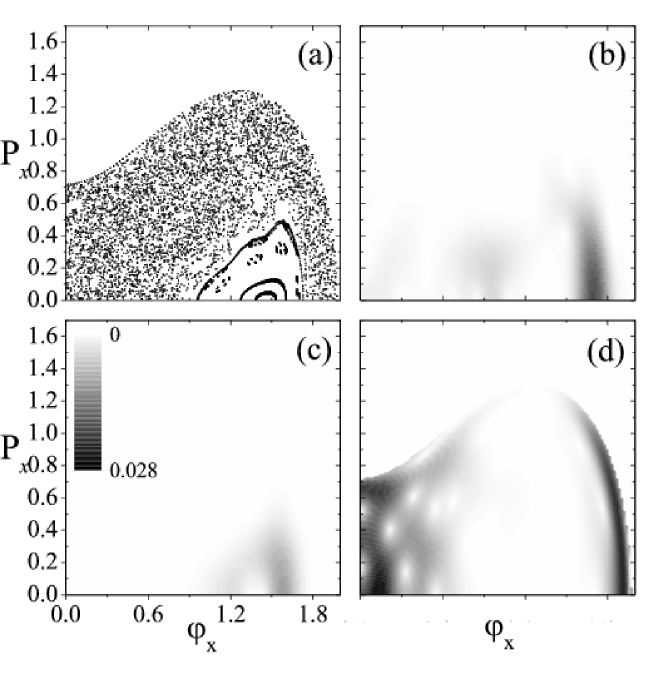
Figure 7: Classical Poincaré surface of section for $E=1.7$. Section of Husimi phase space distribution, $\Phi^{H}_{\nu}(P_{x},\varphi_{x})$ for (b) $E_{\nu}=1.6992$, (c) $E_{\nu}=1.7004$, (d) $E_{\nu}=1.6994$.

V Conclusions

In this paper we have characterized the quantum signatures of chaos in the three-junction SQUID device. For realistic parameter values the classical dynamics exhibits different regimes that go from mixed dynamics to fully developed chaotic motion. As a consequence the spectral statistics, characterized by the distribution of the nearest neigbour energy spacing (NNS) $P(s)$ in the high energy region, is expected to unveil signatures of the mentioned behavior. The analysis has been performed for different energy regions inside the classical intervals corresponding both to the soft chaos (i.e., mixed phase space) and hard chaos regimes, and we considered the even-even parity states to compute the NNS distribution. Our numerical results show that, for $\eta<0.05$ (and for $\eta=0.01$ in particular), in a nearly semiclassical regime, $P(s)$ is well fitted by Berry-Robnik like formulae, where the pure classical measures of the chaotic and regular regions have been used as the only free parameters.

We also found that the individual eigenstates can also be intimately linked to the phase space structures that characterizes the different classical regimes for $\eta<0.05$. In order to analyze how quantum states are supported or localized on different classical structures that are present in the different regimes in this case, we have investigated the Husimi phase space distributions for different eigenstates with energies $E_{\nu}$ in the classical interval. We would like to mention that there are few studies of Husimi distributions for Hamiltonian systems with two degrees of freedom, groh as it is the case of the DFJQ studied in the present work.

One important advantage of Josephson junction devices is that they can be fabricated with well-controlled parameters. The effective $\hbar$, is $\hbar_{\rm eff}=\eta=\sqrt{\frac{8E_{C}}{E_{J}}}$, and since $E_{J}\propto A$ and $E_{C}\propto 1/A$, with $A$ the area of the junctions, we have that $\hbar_{\rm eff}\propto 1/A$. Thus, the fabrication of different DJFQ with junctions with varying area could allow to study cases with $\hbar_{\rm eff}$ spanning from the semiclassical to the quantum regime. This is indeed important since different regimes can be accessed experimentally depending on the magnitude of $\eta$. The qubit regime of two-level dynamics of the DJFQ is observed experimentally in devices with $\eta\approx 0.4$.chiorescu ; fqubit_recent In Ref.mingo, it has been found that signatures of chaos in the Loschmidt echo can be observed at high energies $E\sim 3E_{J}$ in devices with an effective $\hbar$ of the order of $\eta\approx 0.1$. Here we have shown that the observation of the quantum effects in the case with mixed chaotic and regular orbits (for an intermediate energy range) needs the study of devices in a more semiclassical regime with $\eta\approx 0.01$. This could motivate experimental measurements looking for the dependence of the Loschmidt echomingo with initial conditions, due to the phase space structure of the mixed classical dynamics, if the experiments are performed in devices with $\eta\approx 0.01$. Considering the valuesnota of $E_{J}\sim 250GHz\sim 2K$ and the operation temperature of $20$ m$K$ reported by the Delft group chiorescu , typical level spacings of $0.01E_{J}\sim 20$ m$K$ can be experimentally resolved in the device of Ref.chiorescu, . This energy resolution is enough for the case of the Loschmidt echo in devices with $\eta\sim 0.1$, analyzed originally in Ref.mingo, . However, the semiclassical regime explored in this work ($\eta=0.01$) requires a resolution in the level spacings of the order of $5\times 10^{-4}E_{J}$. Thus, for experiments in the cryogenic range ($20$ m$K$) devices with larger values of $E_{J}$ should be employed. On one hand, a smaller $\eta\sim 0.01$ already requires junctions with larger area $A$, and therefore larger $E_{J}$. On the other hand, Josephson junctions fabricated with high $T_{c}$ superconductorsjhtc can have a large $E_{J}$. Therefore, devices designed with high $T_{c}$ superconductors can be good candidates for the experimental challenge of studying the mixed phase space in the semiclassical regime of the DJFQ.

Another possible type of experiment is to start the system in the ground state and apply a constant pulse in some external parameter (for instance, the magnetic field). After the pulse is applied, the probability of remaining in the ground state could be related to the energy level statistics.cohen Also, an interesting experiment could be to perform studies of the low frequency noise, as it has been done in mesoscopic chaotic cavities.buttiker ; beenakker-rmp For example, one could drive the DJFQ into the hard chaos regime with a voltage source such that $E_{V}=\frac{1}{2}CV^{2}>E_{hc}$ (and $V<2\Delta/e$) and then measure the noise in the current. How the current noise is related to the spectral statistics in this case is a very interesting problem, which could be the subject of future studies.

- (1) Y. Nakamura, Y. A. Paskin, J. S. Tsai, Nature 398, 786 (1999).
- (2) J. E. Mooij, T.P.Orlando, L.S. Levitov, L. Tian, C.H. van der Wal and S. Lloyd, Science 285, 1036 (1999); T.P.Orlando, J.E. Mooij, L. Tian, C.H. van der Wal, L.S. Levitov, S. Lloyd, J.J. Mazo, Phys. Rev. B 60, 15398 (1999).
- (3) D. Vion, A. Aassime, A. Cottet, P. Joyez, H. Pothier, C. Urbina, D. Esteve, and M. H. Devoret, Science 296, 886 (2002).
- (4) J. M. Martinis, S. Nam, J. Aumentado and C. Urbina, Phys. Rev. Lett. 89, 117901 (2002); Y. Yu, Y. Yu, S. Han, X. Chu, S.-I. Chu, and Z. Wang, Science 296, 889 (2002).
- (5) Y. Makhlin, G. Schön, and A. Shnirman, Rev. Mod. Phys. 73, 357 (2001).
- (6) I. Chiorescu, Y. Nakamura, C. J. P. M. Harmans, and J. E. Mooij, Science 299, 1869 (2003).
- (7) I. Chiorescu, P. Bertet, K. Semba, Y. Nakamura, C. J. P. M. Harmans, and J. E. Mooij, Nature 431, 159 (2004); E. Il’ichev, N. Oukhanski, A. Izmalkov, Th. Wagner, M. Grajcar, H.-G. Meyer, A. Yu. Smirnov, A. Maassen van den Brink, M. H. S. Amin, and A. M. Zagoskin, Phys. Rev. Lett. 91, 097906 (2003); Y. Yu, D. Nakada, J. C. Lee, B. Singh, D. S. Crankshaw, T. P. Orlando, W. D. Oliver, and K. K. Berggren, Phys. Rev. Lett. 92, 117904 (2004); A. Lupascu, C. J. M. Verwijs, R. N. Schouten, C. J. P. M. Harmans, and J. E. Mooij, Phys. Rev. Lett. 93, 177006 (2004); P. Bertet, I. Chiorescu, G. Burkard, K. Semba, C. J. P. M. Harmans, D. P. DiVincenzo, and J. E. Mooij, Phys. Rev. Lett. 95, 257002 (2005).
- (8) S. Montangero, A. Romito, G. Benenti, and R. Fazio, Europhys. Lett. 71, 893 (2005).
- (9) E. N. Pozzo and D. Domínguez, Phys. Rev. Lett. 98, 057006 (2007).
- (10) R. A. Jalabert and H. M. Pastawski, Phys. Rev. Lett. 86, 2490 (2001).
- (11) M. L. Metha , Random Matrices (Academic Press, San Diego, CA, 1991).
- (12) O. Bohigas, M.J. Giannoni and C. Schmit, Phys. Rev. Lett. 52, 1 (1984).
- (13) M. V. Berry and M. Robnik, J. Phys. A: Math Gen. 17, 2413 (1984).
- (14) T. H. Seligman, J. J. M. Verbaarschot and M. R. Zirnbauer J. Phys. A 18, 2751 (1985); Phys. Rev. Lett. 53, 215 (1984).
- (15) E. Haller, H. Köppel, L. S. Cederbaum, Phys. Rev. Lett. 52, 1665 (1984).
- (16) Th. Zimmermann, H.D. Meyer, H. Köppel, L. S. Cederbaum, Phys. Rev. 33, 4334 (1986).
- (17) T Prosen and M. Robnik, J. Phys. A 27 8059 (1994); T Prosen, J. Phys. A: Math. Gen. 28, L349 (1995); T. Prosen, J. Phys. A 31, 7023 (1998); T. Prosen and M. Robnik, J. Phys. A 32, 1863 (1999); J. Malovrh and T. Prosen, J. Phys. A 35, 2483 (2002).
- (18) H. Makino, T. Harayama, and Y. Aizawa Phys. Rev. E 59, 4026 (1999); H. Makino, T. Harayama, and Y. Aizawa Phys. Rev. E 63, 056203 (2001).
- (19) J. M. G. Gómez, A. Relaño, J. Retamosa, E. Faleiro, L. Salasnich, M. Vranicar, and M. Robnik, Phys. Rev. Lett. 94, 084101 (2005)
- (20) E. P. Wigner, Phys. Rev. 40, 749 (1932).
- (21) K. Husimi, Proc. Phys. Soc. Japan 22, 264 (1940).
- (22) H.-W. Lee, Phys. Rep. 259, 147 (1995).
- (23) G. Groh, H. J. Korsch and W. Schweizer, J. Phys. A: Math. Gen. 31, 6897 (1998).
- (24) P. Leboeuf and A. Voros, J. Phys. A: Math Gen. 23, 1765 (1990).
- (25) M.A. Nielsen, E. Knill and R. Laflamme, Nature (London) 396, 52 (1998).
- (26) C. Miquel, J. P. Paz, M. Saraceno, R. Laflamme, E. Knill and C. Negrevergne, Nature 418, 59 (2002).
- (27) M. W. Mitchell, C. W. Ellenor, S. Schneider and A. M. Steinberg, Phys. Rev. Lett. 91, 120402 (2003).
- (28) J. F. Kanem, S. Maneshi, S. H. Myrskog and A M Steinberg, J. Opt. B: Quantum Semiclass. Opt. 7 S705 (2005) and references therein.
- (29) M. Steffen, M. Ansmann, R. McDermott, N. Katz, R. C. Bialczak, E. Lucero, M. Neeley, E. M. Weig, A. N. Cleland and J. M. Martinis, Phys. Rev. Lett. 97, 050502 (2006).
- (30) B. A. Huberman, J. P. Crutchfield and N. H. Packard, Appl. Phys. Lett. 37, 750 (1980); E. Ben-Jacob, I. Goldhirsch, Y. Imry and S. Fishman, Phys. Rev. Lett. 49, 1599 (1982); R. L. Kautz and R. Monaco, J. Appl. Phys. 57, 875 (1985); R. L. Kautz, Rep. Prog. Phys. 59, 935 (1996).
- (31) M. Octavio and C. R. Nasser, Phys. Rev. B 30, 1586 (1984); M. Iansiti, Q. Hu, R. M. Westervelt and M. Tinkham, Phys. Rev. Lett. 55, 746 (1985); C. Noeldeke, R. Gross, M. Bauer, G. Reiner, H. Seifert J. Low Temp. Phys. 64, 235 (1986).
- (32) R. Bhagavatula, C. Ebner and C. Jayaprakash, Phys. Rev. B 45, 4774 (1992); D. Domínguez and H. A. Cerdeira, Phys. Rev. Lett. 71, 3359 (1993); Phys. Rev. B 52, 513 (1995).
- (33) R. H. Parmenter and L. Y. Yu, Physica D 80, 289 (1995).
- (34) R. Graham, M. Schlautmann, and D. L. Shepelyansky, Phys. Rev. Lett. 67, 255 (1991); R. Graham and J. Keymer, Phys. Rev. A 44, 6281 (1991).
- (35) T. D. Clark, J. F. Ralph, R. J. Prance, H. Prance, J. Diggins and R. Whiteman, Phys. Rev. E 57, 4035 (1998); M. J. Everitt, T. D. Clark, P. B. Stiffell, R. J. Prance, H. Prance, A. Vourdas and J. F. Ralph, Phys. Rev. B 64, 184517 (2001); M. J. Everitt, T. D. Clark, P. B. Stiffell, A. Vourdas, J. F. Ralph, R. J. Prance, and H. Prance, Phys. Rev A 69, 043804 (2004).
- (36) Minimum uncertainty wave packets (i.e., coherent states) are typically used for the numerical computation of the Loschmidt echo as well as for analytical calculations in the semiclassical limit. However, “idealized coherent states” are not needed in a strict sense, and localized wave packets are enough as initial conditions for the experimental observation of the Lyapunov regime of the Loschmidt echo. In Ref.mingo, it is discussed how localized wave packets could be prepared experimentally in the DJFQ.
- (37) J. Liu, W. Wang, C. Zhang, Q. Niu, and B. Li, Phys. Rev. A 72, 063623 (2005).
- (38) T. Kato, K.-I. Tanimoto, and K. Nakamura, Phys. Lett. A 322, 324 (2004).
- (39) In general, the relative importance of the on-site capacitance with respect to the capacitance of the junctions depends on the substrate and the type of junction of the device.
- (40) The Hamiltonian of Eq.(1) is a good approximation to the physics of the Josephson junctions for energies , with the superconducting gap. For example in Ref. chiorescu, Al/AlOx/Al junctions were used. An estimate of the value of the superconducting gap in Al can be obtained from D. C. Ralph, C. T. Black and M. Tinkham, Phys. Rev. Lett. 78, 4087 (1997), where a value of meV is quoted (see the caption of their Fig.3). The value of the Josephson energy quoted in Ref.chiorescu, is 259 GHz = 0.16 meV. This leads to the estimate , and thus the results obtained with the Hamiltonian of Eq.(1) will be valid for . As it can be observed in Fig. 2, the hard chaos regime is well within this limit.
- (41) For an analogous system, see for example R. Ketzmerick, K. Kruse, D. Springsguth, and T. Geisel, Phys. Rev. Lett. 84, 2929 (2000).
- (42) K. K. Likharev, Dynamics of Josephson junctions and circuits (Gordon Breach and Science, New York, 1986).
- (43) G. Schön and A. D. Zaikin, Phys. Rep. 198, 237 (1990).
- (44) M. Iansiti, A. T. Johnson, C. J. Lobb and M. Tinkham, Phys. Rev. Lett. 60, 2414 (1988); S. Corlevi, W. Guichard, F. W. J. Hekking, and D. B. Haviland, Phys. Rev. Lett. 97, 096802 (2006).
- (45) R. Fazio and H. van der Zant, Phys. Rep. 355, 235 (2001).
- (46) L.J. Geerligs, M. Peters, L.E.M. de Groot, A. Verbruggen, J.E. Mooij, Phys. Rev. Lett. 63 326 (1989); H. S. J. van der Zant, W. J. Elion, L. J. Geerligs, and J. E. Mooij, Phys. Rev. B 54, 10081 (1996).
- (47) G. Benettin, L. Galgani, and J.M. Strelcyn, Phys. Rev. A 14, 2338 (1976).
- (48) H. D. Meyer, J. Chem. Phys. 84, 3147 (1986).
- (49) However in some particular systems a non-smooth behavior can be found, see for example P. Cejnar and P. Stransky, Phys. Rev. Lett. 93, 102502 (2004).
- (50) P. Carruthers and M. M. Nieto, Rev. Mod. Phys. 40, 411 (1968); R. Jackiw, J. Math. Phys. 9, 339 (1968).
- (51) T. Bauch, F. Lombardi, F. Tafuri, A. Barone, G. Rotoli, P. Delsing, and T. Claeson, Phys. Rev. Lett. 94, 087003 (2005); K. Inomata, S. Sato, K. Nakajima, A. Tanaka, Y. Takano, H. B. Wang, M. Nagao, H. Hatano, and S. Kawabata, Phys. Rev. Lett. 95, 107005 (2005).
- (52) D. Cohen, F. M. Izrailev, and T. Kottos, Phys. Rev. Lett. 84, 2052 (2000); M. Hiller, D. Cohen, T. Geisel, T. Kottos, Ann. Phys. 321, 1025 (2006).
- (53) Ya. M. Blanter and M. Büttiker, Phys. Rep. 336, 1 (2000).
- (54) C.W.J. Beenakker, Rev. Mod. Phys. 69, 731 (1997).