Transition from a one-dimensional to a quasi-one-dimensional state in interacting quantum wires

Abstract

Upon increasing the electron density in a quantum wire, the one-dimensional electron system undergoes a transition to a quasi-one-dimensional state. In the absence of interactions between electrons, this corresponds to filling up the second subband of transverse quantization, and there are two gapless excitation modes above the transition. On the other hand, strongly interacting one-dimensional electrons form a Wigner crystal, and the transition corresponds to it splitting into two chains (zigzag crystal). The two chains are locked, so their relative motion is gapped, and only one gapless mode remains. We study the evolution of the system as the interaction strength changes, and show that only one gapless mode exists near the transition at any interaction strength.

Transport properties of quantum wires have attracted much attention over recent years Wees ; Thomas ; Reilly ; Cronenwett ; DePicciotto ; Rokhinson ; Auslaender . Due to their quasi-one-dimensional structure, conductance is expected to be quantized in units of the conductance quantum $G_{0}=2e^{2}/h$, where $e$ is the elementary charge and the factor of 2 accounts for spin degeneracy. This property of non-interacting electrons is insensitive to the inclusion of interactions within the Luttinger liquid description. However, a number of experiments show deviations from perfect conductance quantization, such as the so-called 0.7-structure observed below the first plateau Thomas ; Reilly ; Cronenwett ; DePicciotto ; Rokhinson . These experiments have stimulated much theoretical interest in the physics of one-dimensional conductors not captured by the Luttinger-liquid theory, such as that of the spin-incoherent regime characterized by very weak coupling of the electron spins Matveev ; Cheianov ; Fiete . Here we consider another important problem in this category: the transition of the one-dimensional electron system in a quantum wire into a quasi-one-dimensional state.

Whether or not an electron system can be viewed as one-dimensional crucially depends on the strength of interaction us . In the absence of interactions, electrons occupy subbands of transverse quantization, and the system is one-dimensional until the chemical potential reaches the bottom of the second subband. On the other hand, at strong interactions, the electrons form a Wigner crystal, and the subband picture is no longer applicable. The system remains one-dimensional until the interaction energy overcomes the confining potential, and the crystal splits into two chains, forming a zigzag structure Piacente .

There is an obvious difference in the behavior of the system in the vicinity of the transition between the limiting cases of the Wigner crystal at strong interactions on the one hand and non-interacting electrons on the other. In a zigzag Wigner crystal, the two chains are locked, and only one gapless mode (the plasmon) remains. By contrast, in the case of non-interacting electrons the two subbands are independent and therefore represent two gapless modes. In this paper, we address the fate of the gapped mode in the vicinity of the transition as the interaction strength varies. In particular, we show that a gap exists at any interaction strength, Fig. 1. However, the nature of the transition changes as the interaction strength is varied.

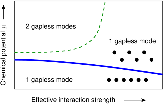
Figure 1: Phase diagram of the electronic system in a quantum wire. The interaction strength can be tuned by varying the confining potential. In the vicinity of the transition to a quasi-one-dimensional state (the lower line) the system supports only one gapless excitation mode at any interaction strength. The state with two gapless excitation modes is expected only at relatively weak interactions.

For simplicity we consider spinless electrons and assume that they interact via long-range Coulomb repulsion,

$$V_{\rm int}=\frac{e^{2}}{2\epsilon}\sum_{k\neq l}\frac{1}{|{\bf r}_{k}-{\bf r}_{l}|}.$$ (1)

Here ${\bf r}_{k}$ are the two-dimensional position vectors of the electrons, and $\epsilon$ is the dielectric constant of the material.

If the electrons in the wire are confined to one dimension by a strong external potential $V_{\rm conf}(y_{k})$, their physics is controlled by the one-dimensional electron density $n_{e}$. Since at $n_{e}\to 0$ the kinetic energy of an electron $\sim(\hbar^{2}/m)n_{e}^{2}$ scales to zero faster than the interaction energy $\sim(e^{2}/\epsilon)n_{e}$, at low densities the Coulomb repulsion dominates. In this limit electrons behave classically. In order to minimize their mutual interaction, they form a periodic one-dimensional structure—the so-called Wigner crystal. At small but finite density, quantum fluctuations smear the long-range order schulz , but the short-range order remains as long as the distance between electrons $n_{e}^{-1}$ is greater than the Bohr radius $a_{B}=\epsilon\hbar^{2}/me^{2}$.

The above picture is valid if the width $w$ of the wire is small, $w\ll a_{B}$. In wider wires, or, equivalently, at stronger interactions, the opposite regime $w\gg a_{B}$ can be achieved. In this case the electrons may form a two-dimensional structure while remaining essentially classical. The structure of the Wigner crystal in this regime can be studied in detail (cf. Ref. Piacente, ), if the confining potential is quadratic,

$$V_{\rm conf}=\frac{1}{2}m\Omega^{2}\sum_{k}y_{k}^{2}.$$ (2)

Here the frequency $\Omega$ determines the width of the wire, $w\sim\sqrt{\hbar/m\Omega}$. The positions of all electrons are found by minimizing the energy $V_{\rm int}+V_{\rm conf}$ over ${\bf r}_{k}$ keeping the one-dimensional electron density $n_{e}$ fixed. The geometry of the classical crystal is controlled by the dimensionless electron density $\nu=n_{e}r_{0}$, where $r_{0}=(2e^{2}/\epsilon m\Omega^{2})^{1/3}$ is the sole length scale of the problem Piacente . At $\nu$ below the critical value $\nu_{c}=\sqrt[3]{4/7\zeta(3)}\approx 0.780$ the energy is minimized when electrons form a one-dimensional crystal, in which $x_{k}=k/n_{e}$ and $y_{k}=0$. At $\nu>\nu_{c}$ the crystal splits into two rows. The distance between rows vanishes at the transition; just above the critical value, when $\delta\nu=\nu-\nu_{c}\ll 1$, it grows as $c=(\sqrt{{24}/{93\zeta(5)}}/\nu_{c}^{2})\sqrt{\delta\nu}$ (in units of $r_{0}$).

Let us consider the low-energy phonons in the zigzag Wigner crystal. Regardless of the density, the crystal has the usual plasmon excitation with acoustic spectrum. In the limit of zero wavevector, this excitation corresponds to translation of the crystal along the wire, $\delta x_{k}=\eta$, $\delta y_{k}=0$ for any $k$. In addition, at the zigzag transition point a transverse soft mode appears, for which $\delta x_{k}=0$ and $\delta y_{k}=(-1)^{k}\varphi$. One can easily show that near the zigzag transition, when $\delta\nu\ll 1$, the coupling of the two low-energy excitation modes is weak, and they can be treated separately. The action describing the soft transverse mode takes the form

$$S=A\hbar\sqrt{\frac{r_{0}}{a_{B}}}\int d\tau\,dx\left[(\partial_{\tau}\varphi)^{2}+(\partial_{x}\varphi)^{2}-\delta\nu\,\varphi^{2}+\varphi^{4}\right].$$ (3)

Here $x$, $\tau$, and the field $\varphi$ have been rescaled so as to yield the simplest form of the action possible. This form, as well as our results from this point on, are not sensitive to the exact shape of the confining potential. In case of the parabolic potential (2) the constant $A=[7\zeta(3)]^{3/2}\sqrt{\ln 2}/31\zeta(5)$.

Above the classical transition point, i.e., at $\delta\nu>0$, the transverse mode becomes unstable. This corresponds to the formation of the zigzag structure. To stabilize the system we keep the quartic term $\varphi^{4}$. Quantum fluctuations affect both the position and the nature of the phase transition. To determine their effect, it is helpful to fermionize the problem. To this end we rediscretize the coordinate $x$ and consider a set of particles moving in a double-well potential $-\lambda\varphi_{j}^{2}+\varphi_{j}^{4}$ with nearest neighbor interaction $(\varphi_{j}-\varphi_{j+1})^{2}$ between them. At sufficiently large $\lambda$ each particle is almost completely localized in one of the minima, and its position can be described by a spin operator, $\varphi_{j}=\pm\sqrt{\lambda/2}=\sqrt{\lambda/2}\,\sigma_{j}^{z}$. In terms of these pseudo-spin variables the Hamiltonian contains two terms: $-t\sum_{j}\sigma^{x}_{j}$ describing tunneling between the two minima of the double-well potential and $-v\sum_{j}\sigma^{z}_{j}\sigma^{z}_{j+1}$ accounting for the nearest-neighbor interactions. Rotating $\sigma^{x}\to-\sigma^{z}$ and applying the Jordan-Wigner transformation, one obtains the Hamiltonian

$${\cal H}_{\rm f}=\sum_{j}\Big{[}2t\,a_{j}^{\dagger}a_{j}-v\Big{(}a_{j}^{\dagger}-a_{j}\Big{)}\Big{(}a_{j+1}^{\dagger}+a_{j+1}\Big{)}\Big{]}.$$ (4)

The above procedure has enabled us to convert the bosonic problem (3) to that of non-interacting spinless fermions (4). Since the number of fermions is not conserved, the Hamiltonian should be diagonalized by performing a Bogoliubov transformation. As a result one easily finds that the excitation spectrum of the Hamiltonian (4) has a gap $\Delta$ that vanishes when $t=v$. We identify this point with the phase transition from the one-dimensional state of the wire at $t>v$ when all the fermionic states in the Hamiltonian (4) are empty, to the quasi-one-dimensional state at $v>t$, in which fermionic states describing the transverse degrees of freedom in the wire are filled, but possess a spectral gap. Near the transition the gap behaves linearly, $\Delta=2|v-t|$.

In experiments with quantum wires, the transition from a one-dimensional to a quasi-one-dimensional state is observed when the chemical potential $\mu$ of electrons is tuned by applying a voltage to the gate controlling the electron density. The parameters $t$ and $v$ of the Hamiltonian (4) are expected to be non-singular functions of $\mu$. The transition occurs at the critical value $\mu_{c}$, defined as a solution of the equation $t(\mu)=v(\mu)$. The gap in the excitation spectrum is then linear in the distance from the transition,

$$\Delta\propto|\mu-\mu_{c}|.$$ (5)

To better understand the nature of this transition, it is helpful to consider the well-known mapping between phase transitions in $d$-dimensional quantum systems and $(d+1)$-dimensional classical models Vaks-Larkin . In particular, the phase transition in the one-dimensional quantum model (3) is equivalent to that in the two-dimensional classical Ising model Polyakov . In this mapping the gap $\Delta$ becomes the inverse correlation length $r_{c}^{-1}$ of the Ising model, and the scaling $r_{c}\propto|T-T_{c}|^{-1}$, well-known from the exact solutions, is equivalent to Eq. (5). The relation between these phase transitions can be made more explicit by noticing that our Hamiltonian (4) essentially coincides with the transfer matrix Mattis of the Ising model near the transition point.

In the discussion leading to the result (5), the interactions in the quantum wire were assumed to be very strong. To explore the fate of the gap as the interaction strength is reduced, we now turn to the case of weak interactions. In this case the transition to the quasi-one-dimensional state occurs when electrons start populating the second subband of transverse quantization in the wire. In this regime one can neglect the presence of the other subbands and present electron wavefunctions as $\psi(x,y)=\psi_{1}(x)\chi_{1}(y)+\psi_{2}(x)\chi_{2}(y),$ where $\chi_{1,2}(y)$ are the first and second eigenstates in the confining potential. Weak interactions between electrons lead to coupling of the two subbands. The low energy properties of the system are described by four interaction constants. The first three constants, $g_{1}$, $g_{2}$, and $g_{x}$, correspond to density-density interactions in the first subband, the second one, and between the two subbands, respectively. The fourth coupling constant $g_{t}$ accounts for the possibility of transfer of pairs of electrons from one subband to the other, Fig. 2(a).

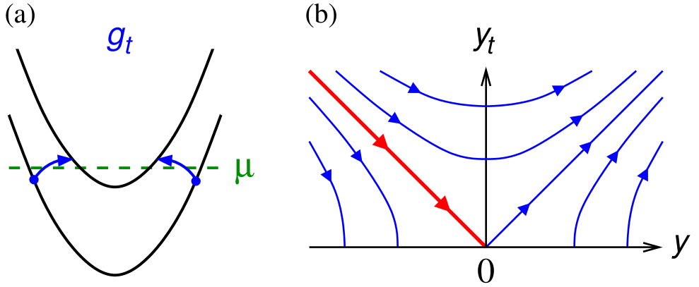
Figure 2: (a) The scattering processes transferring pairs of particles between the two subbands. (b) The flow diagram for the renormalization group (6).

It is well known that in one-dimensional systems density-density couplings renormalize the velocities of the acoustic low-energy excitations, but do not lead to the emergence of spectral gaps Giamarchi . On the other hand, the coupling $g_{t}$ creates and destroys pairs of electrons in each subband and thus can, in principle, lead to a BCS-like gap in the spectrum. Since the coupling constants in weakly interacting one-dimensional electron systems acquire logarithmic renormalizations at low energies Giamarchi , the existence of a gap is determined by the scaling of $g_{t}$.

The renormalization group equations for the four coupling constants have been derived in Ref. Ledermann, . As the bandwidth of the problem is scaled from $D_{0}$ down to $D$, the renormalization of the coupling constants can be found by solving the system of two coupled equations

$$y_{t}^{\prime}=yy_{t},\quad y^{\prime}=y_{t}^{2}.$$ (6)

Here the derivatives are with respect to $\xi=\ln(D_{0}/D)$,

$$y_{t} = \frac{g_{t}}{\pi\hbar}\sqrt{\frac{(v_{F1}+v_{F2})^{2}+4v_{F1}v_{F2}}{2v_{F1}v_{F2}(v_{F1}+v_{F2})^{2}}},$$

$$y = -\frac{1}{2\pi\hbar}\left(\frac{g_{1}}{v_{F1}}+\frac{g_{2}}{v_{F2}}-\frac{4g_{x}}{v_{F1}+v_{F2}}\right),$$

$v_{F1}$ and $v_{F2}$ are the Fermi velocities in the two subbands.

The renormalization group flow corresponding to the equations (6) is shown in Fig. 2(b). To find the initial values of $y_{t}$ and $y$ we compute the coupling constants in first order in the interaction strength. Assuming that the Coulomb interactions between electrons are screened by a gate at distance $d$, in the limit of low electron density in the second subband we find with logarithmic accuracy $g_{1}^{(0)}=g_{x}^{(0)}=2e^{2}\ln(k_{F1}d)$ and $g_{2}^{(0)}\sim e^{2}(k_{F2}d)^{2}\ln(1/k_{F2}d)$. It is important to note that $g_{2}^{(0)}/v_{F2}$ vanishes when approaching the transition. This is a consequence of the Pauli principle. When the average distance between electrons is large, interactions between them are effectively local. Then, as identical fermions never occupy the same place, electrons essentially do not interact. From these estimates we conclude that $y^{(0)}$ is positive, $y^{(0)}\simeq(3e^{2}/\pi\hbar v_{F1})\ln(k_{F1}d)$, and according to the flow diagram Fig. 2(b), the interaction constant $g_{t}$ scales to infinity. Consequently, the system develops a spectral gap. To find its value, we estimate $g_{t}^{(0)}$ near the transition as $g_{t}^{(0)}\sim e^{2}k_{F2}/k_{F1}$ and obtain

$$\Delta\propto(\mu-\mu_{c})^{\alpha}.$$ (7)

Thus the gap in the spectrum of transverse excitations of the wire exists not only when the interactions are strong, but also when they are weak. Unlike the case of strong interactions (5), at weak coupling the power-law dependence (7) has a very large exponent $\alpha=(4y^{(0)})^{-1}\gg 1$.

To gain insight into the evolution of the transition between the two limiting cases, we derive the effective Hamiltonian of the system at intermediate interactions. Since the interactions between electrons in the lower subband are no longer weak and only their properties near the Fermi level are important, it is convenient to use the bosonization approach Giamarchi . On the other hand, as we discussed, near the transition interactions between electrons in the second subband are negligible, $g_{2}\to 0$. Furthermore, the curvature of their spectrum is important in this regime, so the description in terms of fermionic operators is more appropriate. The non-vanishing density-density interactions can still be described by the constants $g_{1}$ and $g_{x}$, although their values may no longer be computed in first-order perturbation theory. Under these conditions the Hamiltonian has the form

$${\cal H} = \frac{\hbar v_{F1}}{2\pi}\int dx\left((\partial\theta)^{2}+\frac{(\partial\phi)^{2}}{K^{2}}\right)-\frac{\hbar^{2}}{2m}\int dx\,\psi^{\dagger}\partial^{2}\psi$$ (8)

$$+\gamma_{t}\int dx\left\{[(\partial\psi)\psi-\psi\partial\psi]e^{2i\kappa\theta(x)}+{\rm h.c.}\right\}.$$

Here the bosonic fields $\phi(x)$ and $\theta(x)$ describe the density excitations in the first subband, $K=(1+g_{1}/\pi\hbar v_{F1})^{-1/2}$ is the respective Luttinger liquid parameter, $\psi$ is the electron destruction operator for the second subband, the constant $\gamma_{t}\sim e^{2}$, and $\kappa=1-K^{2}g_{x}/\pi\hbar v_{F1}$. In deriving Eq. (8) we performed a unitary transformation balents which removed the density-density coupling between the two subbands and changed the phase factor $e^{2i\theta}$ in the last term to $e^{2i\kappa\theta}$.

The Hamiltonian (8) interpolates between the limits of weak and strong interactions. In the weak coupling limit $\kappa\to 1$, and a simple scaling analysis recovers the renormalization group equations (6). At strong interactions the problem of evaluating the coupling constants $g_{1}$ and $g_{x}$ is non-trivial, but in the regime $e^{2}/\hbar v_{F1}\ll 1\ll(e^{2}/\hbar v_{F1})\ln(k_{F1}d)$ one can still use our earlier estimates $g_{1}=g_{x}=2e^{2}\ln(k_{F1}d)$ and conclude that $\kappa\to 0$. Interestingly, in this case the bosonic and fermionic parts of the Hamiltonian (8) decouple, with the latter becoming equivalent to Eq. (4).

One can use the Hamiltonian (8) to discuss the evolution of the gap with varying interaction strength. In the limit of strong interactions, when $\kappa=0$, the magnitude of the pairing term scales to zero near the transition as $k_{F2}$, i.e., slower than the Fermi energy $E_{F2}\propto k_{F2}^{2}$. In this regime, the gap equals the Fermi energy, $\Delta=E_{F2}$, cf. Eq. (5). At strong but finite interactions the pairing term suffers additional power-law suppression at $k_{F2}\to 0$ because of the factor $e^{2i\kappa\theta}$. However, as long as it scales slower than the Fermi energy, the magnitude of the gap remains $\Delta=E_{F2}$. At weaker interactions, when $\kappa$ exceeds a certain critical value, the pairing term scales to zero faster than the Fermi energy. In this regime the gap develops in a small vicinity of the Fermi points, and its dependence on chemical potential is given by a non-universal power law (7) with exponent $\alpha>1$. A more detailed theory of the transition at intermediate interaction strengths will be reported elsewhere unpub .

Our results are summarized in the phase diagram Fig. 1. The electron system in a quantum wire remains one-dimensional and has a single acoustic excitation branch until the chemical potential reaches a certain critical value $\mu_{c}$. At the critical point there is a second gapless mode, and the system can no longer be viewed as one-dimensional. At $\mu>\mu_{c}$ the second mode develops a gap $\Delta\propto(\mu-\mu_{c})^{\alpha}$ with exponent $\alpha=1$ at strong interactions, but very large $\alpha$ at weak coupling. At weak interactions, as the chemical potential is increased further, the residual interactions $g_{2}$ grow, and the gap disappears. This happens when the electron density in the second subband is still very small, of order $(k_{F}d^{2})^{-1}$, long before the third transverse mode appears. We see no physical reason for the gap to disappear at strong coupling. In experiments, the presence of a gap will affect the temperature dependence of the conductance which is expected to show activated behavior even above the transition into the quasi-one-dimensional state. The doubling of the zero-temperature conductance (from $e^{2}/h$ to $2e^{2}/h$ for spinless electrons) occurs at the upper line in Fig. 1.

- (1) B. J. van Wees et al., Phys. Rev. Lett. 60, 848 (1988); D. A. Wharam et al., J. Phys. C 21, L209 (1988).
- (2) O. M. Auslaender et al., Science 308, 88 (2005).
- (3) K. J. Thomas et al., Phys. Rev. Lett. 77, 135 (1996); Phys. Rev. B 61, R13365 (2000).
- (4) D. J. Reilly et al., Phys. Rev. B 63, 121311(R) (2001).
- (5) S. Cronenwett et al., Phys. Rev. Lett. 88, 226805 (2002).
- (6) R. de Picciotto et al., Phys. Rev. B 72, 033319 (2005).
- (7) L. P. Rokhinson, L. N. Pfeiffer, and K. W. West, Phys. Rev. Lett. 96, 156602 (2006).
- (8) K. A. Matveev, Phys. Rev. Lett. 92, 106801 (2004).
- (9) V. V. Cheianov and M. B. Zvonarev, Phys. Rev. Lett. 92, 176401 (2004).
- (10) G. A. Fiete and L. Balents, Phys. Rev. Lett. 93, 226401 (2004).
- (11) See also A. D. Klironomos, J. S. Meyer, and K. A. Matveev, Europhys. Lett. 74, 679 (2006).
- (12) G. Piacente et al., Phys. Rev. B 69, 45324 (2004).
- (13) H. J. Schulz, Phys. Rev. Lett. 71, 1864 (1993).
- (14) V. G. Vaks and A. I. Larkin, Zh. Eksp. Teor. Fiz. 49, 975 (1965) [Sov. Phys. JETP 22, 678 (1966)].
- (15) See, e.g., A. M. Polyakov, Gauge Fields and Strings (Harwood Academic Publishers, 1987).
- (16) D. C. Mattis, Theory of Magnetism (Harper & Row, New York, 1965), Ch. 9.
- (17) See, e.g., T. Giamarchi, Quantum Physics in One Dimension (Clarendon Press, Oxford, 2004).
- (18) U. Ledermann and K. Le Hur, Phys. Rev. B 61, 2497 (2000).
- (19) This result differs from the one obtained in Ref. Ledermann, , where no gap was found at because of the assumption . This choice of the initial conditions is not appropriate in our case.
- (20) L. Balents, Phys. Rev. B 61, 4429 (2000).
- (21) J. S. Meyer and K. A. Matveev, unpublished.