A staggered six-vertex model with non-compact continuum limit

Abstract

The antiferromagnetic critical point of the Potts model on the square lattice was identified by Baxter [1] as a staggered integrable six-vertex model. In this work, we investigate the integrable structure of this model. It enables us to derive some new properties, such as the Hamiltonian limit of the model, an equivalent vertex model, and the structure resulting from the $Z_{2}$ symmetry. Using this material, we discuss the low-energy spectrum, and relate it to geometrical excitations. We also compute the critical exponents by solving the Bethe equations for a large lattice width $N$. The results confirm that the low-energy spectrum is a collection of continua with typical exponent gaps of order $(\log N)^{-2}$.

1 Introduction

Our understanding of $1+1$ conformal field theories with non compact target spaces has improved a great deal in the last few years, thanks to the use of geometrical methods [2], and ideas from string theory [3]. The topic is of the highest interest in the context of the AdS/CFT duality.

Theories with non compact target spaces also play an important role in statistical mechanics. A sophisticated example of this role occurs in the supersymmetric approach to phase transitions for non interacting disordered electronic systems, where the universality class of the transition between plateaux of the integer quantum Hall effect is related with the IR limit of a non compact $1+1$ supersigma model at $\theta=\pi$ [4]. A more basic example is provided by Brownian motion and subtle properties thereof, such as the (non) intersection exponents [5]. In both cases, the non compacity of the target space occurs because the electron trajectories or the random path can visit a given site (edge) an infinite number of times. This is in sharp contrast with self avoiding models for which almost everything is by now understood, and related with ordinary CFTs (essentially, a twisted free boson).

An obvious strategy to tackle the physics of models with non compact target spaces is to start with a lattice model having an infinity of degrees of freedom per site/link. For instance, it is easy to generalize the usual XXX chain to a non compact representation of $SL(2,R)$, and try to use the standard tools of Bethe ansatz, Baxter Q-operator, etc, to obtain properties such as gaplessness and critical exponents. Despite some serious progress in this direction [6], the problem is far from being closed.

Another strategy is based on the observation that a non compact continuum limit may well arise from a lattice model with finite number of degrees of freedom per site/link if the non unitarity is strong enough. The two families of examples exhibited so far involve models with supergroup symmetries—either models with $OSP(m|2n)$ symmetries (such as intersecting loop models) [7] which, in their Goldstone phases can be described in the IR by a collection of free bosons and symplectic fermions, or the $SU(1|2)$ integrable spin chain with alternating $3$ and $\bar{3}$ representations, which was found to be described by the $SU(2|1)$ WZW model at $k=1$ [8]. In both cases, a continuous spectrum of critical exponents is found, and the target space does exhibit some non compact directions indeed.

The examples of Brownian motion and self intersecting dense curves should convince the reader that non compact target spaces are more common and useful than might have been surmised a few years ago. In a recent paper, we found [9] that the antiferromagnetic Potts model on the square lattice for $Q$ continuous has critical properties seemingly involving a twisted non compact boson. This conclusion was based on some numerical and analytical evidence, and implied that the well known six-vertex model itself might exhibit such an exotic continuum limit if properly staggered. The purpose of this paper is to discuss these results further, and put them on considerably firmer grounds.

Indeed, the evidence for a continuous spectrum of critical exponents is not so easy to obtain from studies of a finite lattice model. What was really established so far in [7, 8, 9] was that low energy levels appeared with extremely high degeneracies in the limit of long chains, and that naive calculations of finite size corrections indicated truly infinite degeneracies. This was—thanks to complementary arguments, such as mappings onto sigma models, or abstract construction of WZW theories on supergroups—interpreted as strong indications for a continuous spectrum in the scaling limit. Direct evidence was however missing, together with estimates of the measure of integration on the continuous spectrum, if any. These issues will be resolved here.

The paper is organized as follows. In section 2, the critical antiferromagnetic Potts model and the related staggered six-vertex model are defined. Symmetries and limiting cases are studied. It is shown in particular that the model coincides with the $OSP(2|2)$ model of [7] in one limit, and the $SO(4)$ model in another. In section 3, the solution of the model using the Bethe ansatz is discussed. In section 4, a detailed analysis of the spectrum of conformal exponents from the Bethe equations is carried out. Very accurate evidence for the existence of a continuous spectrum is obtained, together with some information on the measure. This information is used in section 5 to relate the results to theoretical expectations, in particular those of the supersphere sigma model of [10]. Elements for a physical interpretation of the continuous spectrum are proposed in section 6. Conclusions are gathered in section 7.

2 The staggered six-vertex model and its integrable structure

2.1 The general integrable six-vertex model

On the square lattice $\mathcal{L^{\prime}}$ of $2N$ vertical lines and $M$ horizontal lines, associate the complex number $v(J)$ to the $J$-th vertical line, and $h(I)$ to the $I$-th horizontal line (see figure 1). The parameters $v(J)$ and $h(I)$ are called line rapidities.

Figure 1: The spectral parameter $u_{IJ}$ defined by the line rapidities.

On this lattice, define the general inhomogeneous six-vertex model with local weights given in terms of the difference $u_{IJ}=h(I)-v(J)$. The weights that satisfy the Yang-Baxter equations are obtained by taking equations (1.5)–(1.6) of ref. [11] and performing the substitution :

$$t,\rho(I),\sigma(J),\kappa(I,J) \to e^{i\gamma},e^{i\gamma-2ih(I)},e^{2iv(J)},\frac{i}{2}e^{ih(I)-iv(J)-i\gamma}$$ (1)

$$\alpha(I,J),\beta(I,J),\gamma(I,J) \to 1,1,\lambda_{IJ}$$ (2)

Thus, the weights of the inhomogeneous integrable six-vertex model (see figure 2) are :

$$\omega_{1}(I,J),\dots,\omega_{6}(I,J) = \sin\left(\gamma-u_{IJ}\right),\sin\left(\gamma-u_{IJ}\right),\sin u_{IJ},\sin u_{IJ},$$

$$\lambda_{IJ}\ e^{-iu_{IJ}}\sin\gamma,\left(\lambda_{IJ}\right)^{-1}\ e^{iu_{IJ}}\sin\gamma$$ (3)

Figure 2: The allowed configurations of the six-vertex model.

The parameters $\lambda_{IJ}$ must satisfy the additional condition :

$$\lambda_{I,J+1}\lambda_{I+1,J}=\lambda_{I,J}\lambda_{I+1,J+1}$$ (4)

The parameters $\lambda_{IJ}$ do not alter the eigenvalues of the transfer matrix, thus they play the role of gauge parameters. The parameter $\Delta$ has the value :

$$\Delta=-\cos\gamma$$ (5)

2.2 The staggered six-vertex model associated to the critical antiferromagnetic Potts model

The anisotropic Potts model on the square lattice $\mathcal{L}$ is defined by the partition function :

$$Z_{\mathrm{Potts}}=\sum_{\{s_{i}\}}\prod_{\langle ij\rangle\mathrm{even}}\exp\left[J_{1}\delta(s_{i},s_{j})\right]\prod_{\langle ij\rangle\mathrm{odd}}\exp\left[J_{2}\delta(s_{i},s_{j})\right]$$ (6)

where each spin $s_{i}$ lives on a vertex of $\mathcal{L}$ (white circles), and each coupling factor is associated to an edge of $\mathcal{L}$ (dotted lines). The spin $s_{i}$ can take $Q$ distinct values. The sum is over all spin configurations, and each product corresponds to one type of edge of $\mathcal{L}$.

When the couplings $J_{1}$ and $J_{2}$ are negative, the model is antiferromagnetic. In this domain, the critical line separating the paramagnetic and antiferromagnetic phases is given by the condition :

$$\left(e^{J_{1}}+1\right)\left(e^{J_{2}}+1\right)=4-Q$$ (7)

The model defined by eq. (6) on the square lattice $\mathcal{L}$ can be mapped to a six-vertex model on the square lattice $\mathcal{L^{\prime}}$. This lattice is represented in full lines and black circles, and is called the medial lattice of $\mathcal{L}$ (see figure 3).

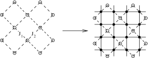
Figure 3: The square lattice $\mathcal{L}$ (dotted lines and white circles) and its medial lattice $\mathcal{L^{\prime}}$ (full lines and black circles).

The weights of this six-vertex model depend on the parameters $J_{1}$, $J_{2}$ and $Q$. We use the notations :

$$\sqrt{Q}=2\cos\gamma$$ (8)

$$x_{1}=\frac{e^{J_{1}}-1}{\sqrt{Q}}\ ,\qquad x_{2}=\frac{e^{J_{2}}-1}{\sqrt{Q}}$$ (9)

The equivalent six-vertex model has weights $\omega_{1},\dots,\omega_{6}$ on the even vertices and $\omega^{\prime}_{1},\dots,\omega^{\prime}_{6}$ on the odd vertices, where :

$$\omega_{1},\dots,\omega_{6} = 1,1,x_{1},x_{1},e^{i\gamma/2}+x_{1}e^{-i\gamma/2},e^{-i\gamma/2}+x_{1}e^{i\gamma/2}$$ (10)

$$\omega^{\prime}_{1},\dots,\omega^{\prime}_{6} = x_{2},x_{2},1,1,e^{-i\gamma/2}+x_{2}e^{i\gamma/2},e^{i\gamma/2}+x_{2}e^{-i\gamma/2}$$ (11)

The parameter $\Delta$ is independent of the parameters $x_{1}$ and $x_{2}$ :

$$\Delta=\frac{\omega_{1}\omega_{2}+\omega_{3}\omega_{4}-\omega_{5}\omega_{6}}{2\omega_{1}\omega_{3}}=\frac{\omega^{\prime}_{1}\omega^{\prime}_{2}+\omega^{\prime}_{3}\omega^{\prime}_{4}-\omega^{\prime}_{5}\omega^{\prime}_{6}}{2\omega^{\prime}_{1}\omega^{\prime}_{3}}=-\cos\gamma$$ (12)

The criticality condition (7) can be parametrized by :

$$x_{1}=\frac{\sin u}{\sin(\gamma-u)}\ ,\qquad x_{2}=-\frac{\cos(\gamma-u)}{\cos u}$$ (13)

When this condition is satisfied, the weights (10)–(11) of the Potts model correspond to a particular case of the integrable six-vertex model (3). The rapidity $v(J)$ is equal to 0 (resp. $\pi/2$) when $J$ is even (resp. odd). The rapidity $h(I)$ is equal to $u$ (resp. $u+\pi/2$) when $I$ is even (resp. odd). This configuration of the line rapidities is shown in figure 4. The gauge parameter is set to $\lambda=e^{i\gamma/2}$ at every vertex.

Figure 4: The line rapidities corresponding to the antiferromagnetic critical point of the Potts model

Thus, the partition function of the Potts model at the antiferromagnetic critical point is described by the two-row transfer matrix of the integrable six-vertex model with the above choice of the rapidities. We call this matrix $\mathcal{T}(u)$ (see figure 5).

Figure 5: The transfer matrix $\mathcal{T}(u)$. The value next to each vertex is the spectral parameter $u_{IJ}$.

2.3 The $\mathcal{R}$-matrix and the thirty-eight-vertex model

2.3.1 Building block : the $R$-matrix of the six-vertex model

Definition. The $R$-matrix of the integrable six-vertex model is defined by its matrix element $R^{\nu\beta}_{\alpha\mu}$ equal to the Boltzmann weight of the configuration shown in fig. 6. Let $V$ be the Hilbert space generated by the vectors $|\uparrow\rangle,|\downarrow\rangle$. Then the $R$-matrix is a linear operator mapping the space $V_{\mu}\otimes V_{\alpha}$ onto $V_{\beta}\otimes V_{\nu}$. The matrix elements of the $R$-matrix with spectral parameter $u_{IJ}=u$ and gauge parameter $\lambda_{IJ}=\lambda$ are the Boltzmann weights (3). In the basis $(|\uparrow\uparrow\rangle,|\uparrow\downarrow\rangle,|\downarrow\uparrow\rangle,|\downarrow\downarrow\rangle)$, the $R$-matrix is :

$$R(u,\lambda)=\left(\begin{array}[]{llll}\sin(\gamma-u)&0&0&0\\ 0&\lambda\ e^{-iu}\sin\gamma&\sin u&0\\ 0&\sin u&\lambda^{-1}\ e^{iu}\sin\gamma&0\\ 0&0&0&\sin(\gamma-u)\end{array}\right)$$ (14)

Figure 6: The $R$ matrix of the six-vertex model.

Figure 7: The Yang-Baxter relation for the six-vertex R-matrix.

Symmetries. The $R$-matrix satisfies the Yang-Baxter equations shown in fig. 7 and the inversion relation :

$$R(u,\lambda)R(-u,\lambda^{-1})=\sin(\gamma-u)\sin(\gamma+u)\ {\mathchoice{\rm 1\mskip-4.0mul}{\rm 1\mskip-4.0mul}{\rm 1\mskip-4.5mul}{\rm 1\mskip-5.0mul}}$$ (15)

It also has the symmetry property :

$$R(u+\pi,\lambda)=-R(u,\lambda)$$ (16)

The $R$-matrix preserves the total magnetization :

$$\sigma^{z}_{\mu}+\sigma^{z}_{\alpha}=\sigma^{z}_{\beta}+\sigma^{z}_{\nu}$$ (17)

Relation to the Temperley-Lieb algebra. When the gauge is set to $\lambda=1$, the $R$-matrix can be written in terms of the Temperley-Lieb generator $E$ :

$$R(u,1)=\sin(\gamma-u)\ {\mathchoice{\rm 1\mskip-4.0mul}{\rm 1\mskip-4.0mul}{\rm 1\mskip-4.5mul}{\rm 1\mskip-5.0mul}}+\sin u\ E$$ (18)

where :

$$E=\left(\begin{array}[]{llll}0&0&0&0\\ 0&e^{-i\gamma}&1&0\\ 0&1&e^{i\gamma}&0\\ 0&0&0&0\end{array}\right)$$ (19)

In the Hilbert space of row configurations $V_{1}\otimes\dots\otimes V_{2N}$, define the operators :

$$E_{m}\equiv{\mathchoice{\rm 1\mskip-4.0mul}{\rm 1\mskip-4.0mul}{\rm 1\mskip-4.5mul}{\rm 1\mskip-5.0mul}}_{1}\otimes\dots\otimes{\mathchoice{\rm 1\mskip-4.0mul}{\rm 1\mskip-4.0mul}{\rm 1\mskip-4.5mul}{\rm 1\mskip-5.0mul}}_{m-1}\otimes E\otimes{\mathchoice{\rm 1\mskip-4.0mul}{\rm 1\mskip-4.0mul}{\rm 1\mskip-4.5mul}{\rm 1\mskip-5.0mul}}_{m+2}\otimes\dots\otimes{\mathchoice{\rm 1\mskip-4.0mul}{\rm 1\mskip-4.0mul}{\rm 1\mskip-4.5mul}{\rm 1\mskip-5.0mul}}_{2N}\ ,\qquad m=1\dots 2N$$ (20)

with a non-trivial action on the space $V_{m}\otimes V_{m+1}$. This family of operators satisfy the Temperley-Lieb algebra :

$$(E_{m})^{2}=\sqrt{Q}\ E_{m}$$ (21)

$$E_{m}=E_{m}E_{m+1}E_{m}=E_{m}E_{m-1}E_{m}$$ (22)

$$E_{m}\ E_{m^{\prime}}=E_{m^{\prime}}\ E_{m}\quad\mathrm{if}\quad|m-m^{\prime}|>1$$ (23)

The operators $E_{m}$ can be expressed in terms of the Pauli matrices :

$$E_{m}=\frac{1}{2}\left[\sigma_{m}^{x}\ \sigma_{m+1}^{x}+\sigma_{m}^{y}\ \sigma_{m+1}^{y}-\cos\gamma(\sigma_{m}^{z}\ \sigma_{m+1}^{z}-{\mathchoice{\rm 1\mskip-4.0mul}{\rm 1\mskip-4.0mul}{\rm 1\mskip-4.5mul}{\rm 1\mskip-5.0mul}})-i\sin\gamma(\sigma_{m}^{z}-\sigma_{m+1}^{z})\right]$$ (24)

or, in a more compact form :

$$E_{m}=\sigma_{m}^{+}\ \sigma_{m+1}^{-}+\sigma_{m}^{-}\ \sigma_{m+1}^{+}+\frac{1}{2}({\mathchoice{\rm 1\mskip-4.0mul}{\rm 1\mskip-4.0mul}{\rm 1\mskip-4.5mul}{\rm 1\mskip-5.0mul}}-\sigma_{m}^{z}\sigma_{m+1}^{z})e^{-i\gamma\sigma_{m}^{z}}$$ (25)

2.3.2 The $\mathcal{R}$-matrix. Conservation laws.

The six-vertex model defined in section 2.2 is not homogeneous, and the transfer matrix $\mathcal{T}(u)$ is built using $R$-matrices with different values of $u_{IJ}$. One can construct a homogeneous model by considering the $\mathcal{R}$-matrix, acting on double-edges. The double-edges live in the Hilbert space :

$$\mathcal{V}\equiv V\otimes V$$ (26)

The $\mathcal{R}$-matrix acts on the product space $\mathcal{V}\otimes\mathcal{V}$.

Figure 8: The matrix $\mathcal{R}(u)$, defining the antiferromagnetic critical point of the Potts model.

As a consequence of the magnetization conservation by $R$, the $\mathcal{R}$-matrix also preserves the total magnetization :

$$\sigma^{z}_{\mu_{1}}+\sigma^{z}_{\mu_{2}}+\sigma^{z}_{\alpha_{1}}+\sigma^{z}_{\alpha_{2}}=\sigma^{z}_{\beta_{1}}+\sigma^{z}_{\beta_{2}}+\sigma^{z}_{\nu_{1}}+\sigma^{z}_{\nu_{2}}$$ (27)

When the gauge parameter is set to $\lambda=1$, another conserved quantity can be constructed. Start from the operator $c$ :

$$c\equiv-(\cos\gamma)^{-1}R(\pi/2,1)=(\cos\gamma)^{-1}R(-\pi/2,1)$$ (28)

This operator can be expressed in terms of the Temperley-Lieb generator :

$$c={\mathchoice{\rm 1\mskip-4.0mul}{\rm 1\mskip-4.0mul}{\rm 1\mskip-4.5mul}{\rm 1\mskip-5.0mul}}-(\cos\gamma)^{-1}E$$ (29)

According to the inversion relation (15), this operator has the property :

$$c^{2}={\mathchoice{\rm 1\mskip-4.0mul}{\rm 1\mskip-4.0mul}{\rm 1\mskip-4.5mul}{\rm 1\mskip-5.0mul}}$$ (30)

The $\mathcal{R}$-matrix obeys the conservation rule :

$$[\mathcal{R}(u),c\otimes c]=0$$ (31)

This is a consequence of the Yang-Baxter equations and the inversion relation, as shown in fig. 9.

Figure 9: A graphical representation of the identity : $(c\otimes c)^{-1}\mathcal{R}(c\otimes c)=\mathcal{R}$.

The eigenvectors of the operator $c$ are :

$$|0\rangle =(2\cos\gamma)^{-1/2}\left(e^{i\gamma/2}|\uparrow\downarrow\rangle-e^{-i\gamma/2}|\downarrow\uparrow\rangle\right)$$ (32)

$$|\overline{0}\rangle =(2\cos\gamma)^{-1/2}\left(e^{-i\gamma/2}|\uparrow\downarrow\rangle+e^{i\gamma/2}|\downarrow\uparrow\rangle\right)$$ (33)

$$|+\rangle =|\uparrow\uparrow\rangle$$ (34)

$$|-\rangle =|\downarrow\downarrow\rangle$$ (35)

The eigenspace associated to the eigenvalue $1$ is $\{|+\rangle,|-\rangle,|0\rangle\}$, and the eigenspace associated to the eigenvalue $-1$ is $\{|\overline{0}\rangle\}$.

2.3.3 Mapping to the 38-vertex model

The coefficients of the $\mathcal{R}$-matrix in the basis :

$$(|+\rangle,|-\rangle,|0\rangle,|\overline{0}\rangle)\otimes(|+\rangle,|-\rangle,|0\rangle,|\overline{0}\rangle)$$ (36)

define the Boltzmann weights of a 38-vertex model on the square lattice (see figure 10). In this vertex model, each edge carries an arrow or a thick line. The state $|+\rangle$ (resp. $|-\rangle$) is represented by an up or right (resp. down or left) arrow. The state $|0\rangle$ is represented by an empty edge, and the state $|\overline{0}\rangle$ by a thick line. Setting :

$$\gamma_{0} = \pi-2\gamma$$ (37)

$$u_{0} = -2u$$ (38)

$$a_{0},b_{0},c_{0} = \sin(\gamma_{0}-u_{0}),\sin u_{0},\sin\gamma_{0}$$ (39)

the weights of the 38-vertex model read :

$$a_{1}^{(1)} = a_{1}^{(8)}=-\frac{1}{4}\left[(c_{0})^{2}+a_{0}b_{0}\right]$$

$$a_{1}^{(2)} = a_{1}^{(4)}=\frac{1}{4}b_{0}c_{0}$$

$$a_{1}^{(3)} = a_{1}^{(5)}=\frac{1}{4}a_{0}c_{0}$$

$$a_{1}^{(6)} = a_{1}^{(7)}=-\frac{1}{4}a_{0}b_{0}$$

$$a_{2}^{(1)} = a_{4}^{(1)}=-\frac{1}{4}e^{-2iu}a_{0}c_{0}$$

$$a_{2}^{(2)} = a_{4}^{(2)}=\frac{1}{4}a_{0}c_{0}$$

$$a_{3}^{(1)} = a_{5}^{(1)}=-\frac{1}{4}e^{2iu}a_{0}c_{0}$$

$$a_{3}^{(2)} = a_{5}^{(2)}=\frac{1}{4}a_{0}c_{0}$$

$$a_{6}^{(1)} = a_{8}^{(1)}=\frac{1}{4}e^{-i(\gamma-2u)}b_{0}c_{0}$$

$$a_{6}^{(2)} = a_{8}^{(2)}=\frac{1}{4}e^{i\gamma}b_{0}c_{0}$$

$$a_{7}^{(1)} = a_{9}^{(1)}=\frac{1}{4}e^{i(\gamma-2u)}b_{0}c_{0}$$

$$a_{7}^{(2)} = a_{9}^{(2)}=\frac{1}{4}e^{-i\gamma}b_{0}c_{0}$$

$$a_{10}^{(1)} = a_{11}^{(1)}=a_{12}^{(1)}=a_{13}^{(1)}=-\frac{1}{4}a_{0}b_{0}$$

$$a_{10}^{(2)} = a_{11}^{(2)}=a_{12}^{(2)}=a_{13}^{(2)}=-\frac{1}{4}a_{0}b_{0}$$

$$a_{14} = a_{15}=-\frac{1}{4}(a_{0})^{2}$$

$$a_{16} = a_{17}=-\frac{1}{4}(b_{0})^{2}$$

$$a_{18} = \frac{1}{4}e^{-2iu}c_{0}(b_{0}-a_{0})$$

$$a_{19} = \frac{1}{4}e^{2iu}c_{0}(b_{0}-a_{0})$$

Figure 10: The 38-vertex model

2.3.4 The limit $\gamma\to\pi/2$

If the parameter $\gamma$ is set to $\pi/2$ and the spectral parameter $u$ is fixed, then the weights of the 38-vertex model are equal to zero, except :

$$a_{1}^{(1)}=a_{1}^{(8)}=a_{1}^{(6)}=a_{1}^{(7)}=\frac{1}{4}\sin^{2}2u$$

$$a_{10}^{(1,2)}=a_{11}^{(1,2)}=a_{12}^{(1,2)}=a_{13}^{(1,2)}=\frac{1}{4}\sin^{2}2u$$

$$a_{14}=a_{15}=a_{16}=a_{17}=-\frac{1}{4}\sin^{2}2u$$

The $\mathcal{R}$-matrix is proportional to the “graded permutation” $P$ :

$$\mathcal{R} = \frac{1}{4}\sin^{2}2u\ P\qquad(\gamma\to\pi/2,u\ \mathrm{fixed})$$ (40)

$$P|j\rangle|k\rangle = (-1)^{g_{j}g_{k}}|k\rangle|j\rangle\ ,\qquad j,k\in\{0,\overline{0},+,-\}$$ (41)

$$g_{0},g_{\overline{0}},g_{+},g_{-} = 0,0,1,1$$ (42)

This trivial limit can be avoided by scaling the spectral parameter as :

$$\gamma=\frac{\pi}{2}+\epsilon\ ,\qquad u=\frac{\pi}{2}+\epsilon w$$ (43)

where $\epsilon\to 0^{-}$ and $w$ is fixed. In this rescaled limit, the Boltzmann weights are proportional to $\epsilon^{2}$.

Note that the states $|0\rangle,|\overline{0}\rangle$ become degenerate, but the following combinations remain non-degenerate :

$$|0\rangle+i|\overline{0}\rangle = e^{i\pi/4}\left[\tan(-\epsilon/2)\right]^{-1/2}(|\uparrow\downarrow\rangle+i|\downarrow\uparrow\rangle)$$ (44)

$$|0\rangle-i|\overline{0}\rangle = e^{-i\pi/4}\left[\tan(-\epsilon/2)\right]^{1/2}(|\uparrow\downarrow\rangle-i|\downarrow\uparrow\rangle)$$ (45)

Denote $\tilde{a}_{i}^{(j)}$ the matrix elements of $\tilde{\mathcal{R}}\equiv\mathcal{R}/(-\epsilon^{2})$ in the basis $(|0\rangle,|\overline{0}\rangle,|+\rangle,|-\rangle)$. One gets :

$$\tilde{a}_{1}^{(1)}=\tilde{a}_{1}^{(8)}=(1+w-w^{2})$$

$$\tilde{a}_{1}^{(2)}=\tilde{a}_{1}^{(4)}=w$$

$$\tilde{a}_{1}^{(3)}=\tilde{a}_{1}^{(5)}=\tilde{a}_{2}^{(1,2)}=\tilde{a}_{3}^{(1,2)}=\tilde{a}_{4}^{(1,2)}=\tilde{a}_{5}^{(1,2)}=(1-w)$$

$$\tilde{a}_{1}^{(6)}=\tilde{a}_{1}^{(7)}=\tilde{a}_{10}^{(1,2)}=\tilde{a}_{11}^{(1,2)}=\tilde{a}_{12}^{(1,2)}=\tilde{a}_{13}^{(1,2)}=w(1-w)$$

$$\tilde{a}_{6}^{(1,2)}=\tilde{a}_{8}^{(1,2)}=iw$$

$$\tilde{a}_{7}^{(1,2)}=\tilde{a}_{9}^{(1,2)}=-iw$$

$$\tilde{a}_{14}=\tilde{a}_{15}=(1-w)^{2}$$

$$\tilde{a}_{16}=\tilde{a}_{17}=w^{2}$$

$$\tilde{a}_{18}=\tilde{a}_{19}=(1-2w)$$

These weights can be related to an integrable loop model with $OSP(2|2)$ symmetry. Indeed, the matrix $\tilde{\mathcal{R}}$ can be expressed as a combination of the identity, the permutation operator $P$ defined in equation (41), and the Temperley-Lieb operator $E$. The latter is defined in tensor notation as a contraction of the spaces $\mathcal{V}_{\mu},\mathcal{V}_{\alpha}$ and $\mathcal{V}_{\beta},\mathcal{V}_{\nu}$ (see figure 8) :

$$E_{\alpha\mu}^{\nu\beta}=J_{\nu\beta}(J^{\dagger})_{\alpha\mu}$$ (46)

where $J$ is the bilinear form in the basis $(|0\rangle,|\overline{0}\rangle,|+\rangle,|-\rangle)$ :

$$J=\left(\begin{array}[]{rrcr}1&0&0&0\\ 0&1&0&0\\ 0&0&0&i\\ 0&0&-i&0\end{array}\right)\ ,\qquad J^{\dagger}J=JJ^{\dagger}={\mathchoice{\rm 1\mskip-4.0mul}{\rm 1\mskip-4.0mul}{\rm 1\mskip-4.5mul}{\rm 1\mskip-5.0mul}}$$ (47)

By construction, the operator obeys the Temperley-Lieb algebraic relations (21), (22), (23), with :

$$E^{2}=\mathrm{Tr}(J^{*}J)\ E=0$$ (48)

In the block $\{|0\rangle\otimes|0\rangle,|\overline{0}\rangle\otimes|\overline{0}\rangle,|+\rangle\otimes|-\rangle,|-\rangle\otimes|+\rangle\}$, the matrix of the operator $E$ is :

$$E=\left(\begin{array}[]{rrrr}1&1&-i&i\\ 1&1&-i&i\\ -i&-i&-1&1\\ i&i&1&-1\end{array}\right)$$ (49)

The matrix $\tilde{\mathcal{R}}$ is equal to :

$$\tilde{\mathcal{R}}=(1-w){\mathchoice{\rm 1\mskip-4.0mul}{\rm 1\mskip-4.0mul}{\rm 1\mskip-4.5mul}{\rm 1\mskip-5.0mul}}+wE+w(1-w)P$$ (50)

These weights define an integrable loop model [12], with three allowed vertices, and a loop fugacity $q=0$. The graphical correspondence is shown in figure 11. Note that according to equation (13), the Potts model is isotropic when $u=\gamma/2+\pi/4$, which is equivalent to $w=1/2$. This is also the isotropic point of the loop model (50).

Figure 11: The three allowed vertices of the dense intersecting loop model.

We conclude that, in the limit $\gamma\to\pi/2$, the staggered six-vertex model coincides with the $OSP(2|2)$ integrable model. In this limit, the arrows represent the fermionic coordinates, and the thin and thick lines the bosonic ones. The equivalence in the boundary conditions has to be treated with some care however: the periodic vertex model corresponds to the antiperiodic sector of the $OSP$ system, with an effective central charge $c_{\mathrm{eff}}=1+(-2)-24\times(-1/8)=2$. This means that the $OSP$ symmetry is broken in the periodic vertex model, where the fermions are twisted - i.e. they become a complex (Dirac) fermion instead of symplectic fermions.

2.3.5 The limit $\gamma\to 0$

The approach for this limit is similar to the case $\gamma\to\pi/2$. Consider the following limit :

$$\gamma=\epsilon\ ,\qquad u=-w\epsilon$$ (51)

where $\epsilon\to 0^{+}$ and $w$ is fixed. It is convenient to perform the change of basis :

$$|\tilde{0}\rangle =i|0\rangle$$ (52)

$$|\tilde{\overline{0}}\rangle =i|\overline{0}\rangle$$ (53)

$$|\tilde{+}\rangle =|+\rangle$$ (54)

$$|\tilde{-}\rangle =|-\rangle$$ (55)

Define a transformation of the $\mathcal{R}$-matrix that does not affect the partition function : the Boltzmann weights of the vertices are multiplied by $(-1)$ for each $\pi/2$-turn of the thick lines (the weight $a_{1}^{(8)}$ is not affected). Since the number of such turns is even for every thick polygon on the lattice, the partition function is invariant under this transformation.

Denote $\tilde{a}_{i}^{(j)}$ the matrix elements of the (rescaled) resulting matrix $\tilde{\mathcal{R}}\equiv\mathcal{R}/(-\epsilon^{2})$ in the basis $(|\tilde{0}\rangle,|\tilde{\overline{0}}\rangle,|\tilde{+}\rangle,|\tilde{-}\rangle)$. One gets :

$$\tilde{a}_{1}^{(1)}=\tilde{a}_{1}^{(8)}=(1+w+w^{2})$$

$$\tilde{a}_{1}^{(2)}=\tilde{a}_{1}^{(4)}=-w$$

$$\tilde{a}_{1}^{(3)}=\tilde{a}_{1}^{(5)}=\tilde{a}_{2}^{(1,2)}=\tilde{a}_{3}^{(1,2)}=\tilde{a}_{4}^{(1,2)}=\tilde{a}_{5}^{(1,2)}=(1+w)$$

$$\tilde{a}_{1}^{(6)}=\tilde{a}_{1}^{(7)}=\tilde{a}_{10}^{(1,2)}=\tilde{a}_{11}^{(1,2)}=\tilde{a}_{12}^{(1,2)}=\tilde{a}_{13}^{(1,2)}=w(1+w)$$

$$\tilde{a}_{6}^{(1,2)}=\tilde{a}_{8}^{(1,2)}=-w$$

$$\tilde{a}_{7}^{(1,2)}=\tilde{a}_{9}^{(1,2)}=-w$$

$$\tilde{a}_{14}=\tilde{a}_{15}=(1+w)^{2}$$

$$\tilde{a}_{16}=\tilde{a}_{17}=w^{2}$$

$$\tilde{a}_{18}=\tilde{a}_{19}=1$$

The corresponding loop model is constructed with two generators $P$ and $E$. The permutation operator $P$ is defined as :

$$P_{\beta\nu\mu\alpha}=\delta_{\beta\alpha}\delta_{\nu\mu}$$ (56)

The Temperley-Lieb operator $E$ with parameter $\sqrt{Q}=4$ is built using the simple contraction :

$$E_{\beta\nu\mu\alpha}=J_{\nu\beta}J_{\alpha\mu}$$ (57)

where :

$$J=\left(\begin{array}[]{rrcr}1&0&0&0\\ 0&1&0&0\\ 0&0&0&1\\ 0&0&1&0\end{array}\right)\ ,\qquad J^{2}={\mathchoice{\rm 1\mskip-4.0mul}{\rm 1\mskip-4.0mul}{\rm 1\mskip-4.5mul}{\rm 1\mskip-5.0mul}}$$ (58)

The matrix $\tilde{\mathcal{R}}$ is equal to :

$$\tilde{\mathcal{R}}=(1+w){\mathchoice{\rm 1\mskip-4.0mul}{\rm 1\mskip-4.0mul}{\rm 1\mskip-4.5mul}{\rm 1\mskip-5.0mul}}-wE+w(1+w)P$$ (59)

These are the integrable weights of the loop model defined in [12] with a loop fugacity $q=4$. Note that, in this regime, the Potts model is anisotropic for any value of $w$. The loop model itself is isotropic when $w=-1/2$ : the relative weight for loop crossings is then equal to $-1/2$. Following [12], this model is a graphical version of the $SO(4)$ integrable model based on the vector representation. Using that $so(4)=sl(2)+sl(2)$ one can expect it to decouple into two copies of the isotropic six-vertex model or XXX spin chain, a feature we will confirm when discussing the associated hamiltonian or Bethe equations.

2.4 Transfer matrices

In this section, we set the gauge to $\lambda=1$, so that the transfer matrices can be related to the generators of the Temperley-Lieb algebra.

One-row transfer matrix. The two-row transfer matrix $\mathcal{T}(u)$ is the product of two one-row transfer matrices : $\mathcal{T}(u)=T(u+\pi/2)\ T(u)$. (see fig. 5). As a consequence of the Yang-Baxter equations and the inversion relation, when periodic boundar conditions are imposed in the horizontal direction, the one-row transfer matrices commute :

$$[T(u),T(u^{\prime})]=0$$ (60)

The one-row transfer matrices have the property :

$$T(u+\pi/2)=(-1)^{N}e^{iP}T(u)e^{-iP}$$ (61)

Define the operator $e^{-iP}$ as the shift of all vertical edges by one site to the right. The operator $c$ defined by equation (28) is used to build a conserved quantity of the transfer matrix. Denoting $c_{m}$ the charge operator acting on the space $V_{m}\otimes V_{m+1}$, the global charge is :

$$C\equiv c_{1}\times c_{3}\times\dots\times c_{2N-1}$$ (62)

$$C^{2}={\mathchoice{\rm 1\mskip-4.0mul}{\rm 1\mskip-4.0mul}{\rm 1\mskip-4.5mul}{\rm 1\mskip-5.0mul}}$$ (63)

If $u=0$, the transfer matrices $T(u),T(u+\pi/2)$ become :

$$T(0)=\left(\frac{1}{2}\sin 2\gamma\right)^{N}\ e^{-iP}\ C$$ (64)

$$T(\pi/2)=\left(-\frac{1}{2}\sin 2\gamma\right)^{N}\ C\ e^{-iP}$$ (65)

The matrices (62), (64), (65) are represented in figure 12.

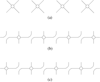
Figure 12: Diagrams defining the transfer matrices $C$ (a), $e^{-iP}C$ (b) and $Ce^{-iP}$ (c), for $N=4$. The white circles represent $c$ operators.

Conservation laws for $\mathcal{T}$. As a consequence of the conservation of the total magnetization and the “charge” $c$ by the $\mathcal{R}$-matrix, the transfer matrix $\mathcal{T}$ preserves the total magnetization :

$$S=\frac{1}{2}(\sigma^{z}_{1}+\dots+\sigma^{z}_{2N})$$ (66)

and the “charge” $C$ defined above. Since $\mathcal{T}(u)$ also commutes with the transfer matrix $T(0)$, $\mathcal{T}(u)$ is invariant under the action of the one-site shift operator $e^{-iP}$.

2.5 Hamiltonian limit of the transfer matrix

To compute the derivative of the matrix $T(u)$ at the points $u=0,u=\pi/2$, it is convenient to write this matrix in terms of the $R$-matrix :

$$T^{\beta_{1}\dots\beta_{2N}}_{\alpha_{1}\dots\alpha_{2N}}(u)=\sum_{\mu_{1},\dots,\mu_{2N}}R^{\mu_{2}\beta_{1}}_{\alpha_{1}\mu_{1}}(u)R^{\mu_{3}\beta_{2}}_{\alpha_{2}\mu_{2}}(u-\pi/2)\dots R^{\mu_{2N}\beta_{2N-1}}_{\alpha_{2N-1}\mu_{2N-1}}(u)R^{\mu_{1}\beta_{2N}}_{\alpha_{2N}\mu_{2N}}(u-\pi/2)$$

Denote by $\delta$ the derivative with respect to $u$. According to eq. (18) :

$$\delta R(u)=-\cos(\gamma-u){\mathchoice{\rm 1\mskip-4.0mul}{\rm 1\mskip-4.0mul}{\rm 1\mskip-4.5mul}{\rm 1\mskip-5.0mul}}+\cos u\ E$$ (67)

Differentiating the previous expression yields :

$$\delta T(0)=\left(\frac{1}{2}\sin 2\gamma\right)^{N-1}\sum_{j=1}^{N}(-\cos^{2}\gamma\ t_{2j-1}+\sin^{2}\gamma\ t_{2j})$$ (68)

where the matrices $t_{2j-1}$ and $t_{2j}$ are defined by the diagrams on fig. 13. Using the graphical representation of the matrices $T(0),t_{2j-1},t_{2j}$ in figures 12–13 and the property (30), one gets the intermediate results :

$$\left[T(0)\right]^{-1}t_{2j-1} = \left(\frac{1}{2}\sin 2\gamma\right)^{-1}c_{V_{2j-3}\otimes V_{2j-2}}\ c_{V_{2j-2}\otimes V_{2j-1}}\ c_{V_{2j-3}\otimes V_{2j-2}}$$ (69)

$$\left[T(0)\right]^{-1}t_{2j} = \left(\frac{1}{2}\sin 2\gamma\right)^{-1}c_{V_{2j-1}\otimes V_{2j}}$$ (70)

The Hamiltonians $H_{1},H_{2}$ are defined as the logarithmic derivatives of the transfer matrix $T(u)$ at the points $u=0,\pi/2$.

$$H_{1} \equiv \frac{1}{2}\sin 2\gamma\ [T(0)]^{-1}\delta T(0)$$

$$= \sum_{j=1}^{N}[-\cos 2\gamma\ {\mathchoice{\rm 1\mskip-4.0mul}{\rm 1\mskip-4.0mul}{\rm 1\mskip-4.5mul}{\rm 1\mskip-5.0mul}}+\cos\gamma\ (E_{2j-1}+E_{2j})-(E_{2j}E_{2j-1}+E_{2j-1}E_{2j})]$$

(71)

Using eq. (61),

$$H_{2} \equiv \frac{1}{2}\sin 2\gamma\ [T(\pi/2)]^{-1}\delta T(\pi/2)$$

$$= e^{iP}H_{1}e^{-iP}$$

$$= \sum_{j=1}^{N}[-\cos 2\gamma\ {\mathchoice{\rm 1\mskip-4.0mul}{\rm 1\mskip-4.0mul}{\rm 1\mskip-4.5mul}{\rm 1\mskip-5.0mul}}+\cos\gamma\ (E_{2j}+E_{2j+1})\ -(E_{2j+1}E_{2j}+E_{2j}E_{2j+1})]$$

(72)

The Hamiltonian associated with the two-row transfer matrix $\mathcal{T}(u)$ is defined as :

$$\mathcal{H}\equiv\frac{1}{2}\sin 2\gamma\ [\mathcal{T}(0)]^{-1}\delta\mathcal{T}(0)$$ (73)

According to the commutation relations (60),

$$\mathcal{H} = H_{1}+H_{2}$$

$$= \sum_{m=1}^{2N}[-\cos 2\gamma\ {\mathchoice{\rm 1\mskip-4.0mul}{\rm 1\mskip-4.0mul}{\rm 1\mskip-4.5mul}{\rm 1\mskip-5.0mul}}+2\cos\gamma\ E_{m}-(E_{m+1}E_{m}+E_{m}E_{m+1})]$$ (74)

Note that the Hamiltonian $\mathcal{H}$ is the sum of two commuting parts :

$$\mathcal{H}=H_{1}+H_{2}\ ,\qquad[H_{1},H_{2}]=0$$ (75)

A consistent decomposition of the momentum operator is :

$$e^{-2iP}=(e^{-iP}C)\times(Ce^{-iP})=(Ce^{-iP})\times(e^{-iP}C)$$ (76)

Indeed, the operators $H_{1},H_{2},(e^{-iP}C),(Ce^{-iP})$ all commute with one another.

Figure 13: Diagrams defining $t_{2j-1}$ and $t_{2j}$ of eq. (68), for $N=4$ and $j=3$. The white circles represent $c$ operators. The arrow points to the vertex that differs from $T(0)$.

Using the expression (25) of the Temperley-Lieb generators, the Hamiltonian (74) is expressed in terms of Pauli matrices :

$$\mathcal{H} = \sum_{m=1}^{2N}\big{[}-(\sigma_{m}^{+}\sigma_{m+2}^{-}+\sigma_{m}^{-}\sigma_{m+2}^{+})+\sin^{2}\gamma\ \sigma_{m}^{z}\sigma_{m+1}^{z}-\frac{1}{2}\sigma_{m}^{z}\sigma_{m+2}^{z}$$ (77)

$$+i\sin\gamma\ (\sigma_{m-1}^{z}-\sigma_{m+2}^{z})(\sigma_{m}^{+}\sigma_{m+1}^{-}+\sigma_{m}^{-}\sigma_{m+1}^{+})-\frac{1}{2}\cos 2\gamma\ {\mathchoice{\rm 1\mskip-4.0mul}{\rm 1\mskip-4.0mul}{\rm 1\mskip-4.5mul}{\rm 1\mskip-5.0mul}}\big{]}$$

In the limit $\gamma\to 0$, the Hamiltonian (77) describes, as expected from the $SO(4)$ identification, two decoupled ferromagnetic XXX spin-chains :

$$\mathcal{H}=-\frac{1}{2}\sum_{j=1}^{N}(\overrightarrow{\sigma}_{2j-1}\cdot\overrightarrow{\sigma}_{2j+1}+{\mathchoice{\rm 1\mskip-4.0mul}{\rm 1\mskip-4.0mul}{\rm 1\mskip-4.5mul}{\rm 1\mskip-5.0mul}})-\frac{1}{2}\sum_{j=1}^{N}(\overrightarrow{\sigma}_{2j}\cdot\overrightarrow{\sigma}_{2j+2}+{\mathchoice{\rm 1\mskip-4.0mul}{\rm 1\mskip-4.0mul}{\rm 1\mskip-4.5mul}{\rm 1\mskip-5.0mul}})\qquad(\gamma=0)$$ (78)

3 Bethe equations, Bethe states and eigenvalues

When periodic conditions are imposed in the horizontal direction, the staggered six-vertex model is solvable by Bethe ansatz [11]. We call $r$ the total number of particles.

3.1 Bethe equations for two types of particles

The Bethe ansatz equations are :

$$\forall j\in\{1,\dots,r\}\qquad\exp\left[2iNk(\alpha_{j})\right]=-\prod_{l=1}^{r}\exp\left[-i\phi(\alpha_{j},\alpha_{l})\right]$$ (79)

The one-particle momentum and the scattering amplitude are given by :

$$\exp\left[2ik(\alpha)\right]=\frac{\sinh(\alpha+i\gamma)}{\sinh(\alpha-i\gamma)}$$ (80)

$$\exp\left[i\phi(\alpha,\alpha^{\prime})\right]=\frac{\sinh\frac{1}{2}(\alpha-\alpha^{\prime}-2i\gamma)}{\sinh\frac{1}{2}(\alpha-\alpha^{\prime}+2i\gamma)}$$ (81)

The roots $\alpha_{j}$ describing the ground state and the physical excitations are expected to sit on the two lines $\mathrm{Im}(\alpha)=\pm\pi/2$. Define two types of particles :

$$\alpha_{j}^{+} = \lambda_{j}+i\pi/2,\qquad j=1,\dots r_{+}$$ (82)

$$\alpha_{j}^{-} = \mu_{j}-i\pi/2,\qquad j=1,\dots r_{-}$$ (83)

The one-particle momenta are :

$$\exp\left[2i\tilde{k}(\lambda)\right]\equiv\exp\left[2ik\left(\lambda\pm i\frac{\pi}{2}\right)\right]=\frac{\cosh(\lambda+i\gamma)}{\cosh(\lambda-i\gamma)}$$ (84)

The scattering amplitude between two particles of the same type is :

$$\exp\left[i\phi_{1}(\lambda,\lambda^{\prime})\right]\equiv\exp\left[i\phi\left(\lambda\pm i\frac{\pi}{2},\lambda^{\prime}\pm i\frac{\pi}{2}\right)\right]=\frac{\sinh\frac{1}{2}(\lambda-\lambda^{\prime}-2i\gamma)}{\sinh\frac{1}{2}(\lambda-\lambda^{\prime}+2i\gamma)}$$ (85)

The scattering amplitude between two particles of different types is :

$$\exp\left[i\phi_{-1}(\lambda,\lambda^{\prime})\right]\equiv\exp\left[i\phi\left(\lambda\pm i\frac{\pi}{2},\lambda^{\prime}\mp i\frac{\pi}{2}\right)\right]=\frac{\cosh\frac{1}{2}(\lambda-\lambda^{\prime}-2i\gamma)}{\cosh\frac{1}{2}(\lambda-\lambda^{\prime}+2i\gamma)}$$ (86)

Define the shifted scattering amplitudes as odd functions of $(\lambda-\lambda^{\prime})$ :

$$\exp\left[i\Theta_{1}(\lambda,\lambda^{\prime})\right]=-\exp\left[i\phi_{1}(\lambda,\lambda^{\prime})\right]$$ (87)

$$\exp\left[i\Theta_{-1}(\lambda,\lambda^{\prime})\right]=\exp\left[i\phi_{-1}(\lambda,\lambda^{\prime})\right]$$ (88)

The Bethe equations (79) split into two sets :

$$\forall j\in\{1,\dots,r_{+}\}\quad e^{2iN\tilde{k}(\lambda_{j})}=(-1)^{r_{+}-1}\prod_{l=1}^{r_{+}}e^{-i\Theta_{1}(\lambda_{j},\lambda_{l})}\prod_{l=1}^{r_{-}}e^{-i\Theta_{-1}(\lambda_{j},\mu_{l})}$$ (89)

$$\forall j\in\{1,\dots,r_{-}\}\quad e^{2iN\tilde{k}(\mu_{j})}=(-1)^{r_{-}-1}\prod_{l=1}^{r_{+}}e^{-i\Theta_{-1}(\mu_{j},\lambda_{l})}\prod_{l=1}^{r_{-}}e^{-i\Theta_{1}(\mu_{j},\mu_{l})}$$ (90)

Take the logarithm of equations (89)–(90) :

$$\forall j\in\{1,\dots,r_{+}\}\quad 2N\tilde{k}(\lambda_{j})=2\pi I_{j}^{+}-\sum_{l=1}^{r_{+}}\Theta_{1}(\lambda_{j},\lambda_{l})-\sum_{l=1}^{r_{-}}\Theta_{-1}(\lambda_{j},\mu_{l})$$ (91)

$$\forall j\in\{1,\dots,r_{-}\}\quad 2N\tilde{k}(\mu_{j})=2\pi I_{j}^{-}-\sum_{l=1}^{r_{+}}\Theta_{-1}(\mu_{j},\lambda_{l})-\sum_{l=1}^{r_{-}}\Theta_{1}(\mu_{j},\mu_{l})$$ (92)

The “Bethe integers” $I_{j}^{\pm}$ follow the following rules : if $r_{+}$ (resp. $r_{-}$) is even, then all the $I_{j}^{+}$ (resp. $I_{j}^{-}$) are half-odd integers; if $r_{+}$ (resp. $r_{-}$) is odd, then all the $I_{j}^{+}$ (resp. $I_{j}^{-}$) are integers. Summing equations (91)–(92) over $j$ and recalling that the functions $\Theta_{\pm 1}$ are odd, one relates the total momentum to the Bethe integers :

$$k_{\mathrm{tot}}=\sum_{j=1}^{r_{+}}\tilde{k}(\lambda_{j})+\sum_{j=1}^{r_{-}}\tilde{k}(\mu_{j})=\frac{\pi}{N}\left(\sum_{j=1}^{r_{+}}I^{+}_{j}+\sum_{j=1}^{r_{-}}I^{-}_{j}\right)$$ (93)

The one-particle momenta and the scattering amplitudes can be written :

$$\tan\left[\tilde{k}(\lambda)\right]=\tanh\lambda\ \tan\gamma$$ (94)

$$\tan\left[\frac{\Theta_{1}(\lambda,\lambda^{\prime})}{2}\right]=\tanh\frac{1}{2}(\lambda-\lambda^{\prime})\ \mathrm{cotan}\gamma$$ (95)

$$\tan\left[\frac{\Theta_{-1}(\lambda,\lambda^{\prime})}{2}\right]=-\tanh\frac{1}{2}(\lambda-\lambda^{\prime})\ \tan\gamma$$ (96)

3.2 Bethe states

Form of the Bethe states. The one-particle states $\varphi_{\alpha}$ are “inhomogeneous plane-waves”, represented in real space as :

$$\varphi_{\alpha}(2m-1) = \cosh\frac{1}{2}(\alpha-i\gamma)\ e^{2ik(\alpha)m}$$ (97)

$$\varphi_{\alpha}(2m) = -\sinh\frac{1}{2}(\alpha+i\gamma)\ e^{2ik(\alpha)m}$$ (98)

with $m=1,\dots,N$ defines the position of the particle. The general Bethe state is given by the linear combination :

$$\varphi_{\alpha_{1},\dots,\alpha_{r}}(x_{1},\dots,x_{r})=\sum_{P}A_{p_{1},\dots,p_{r}}\varphi_{\alpha_{p_{1}}}(x_{1})\dots\varphi_{\alpha_{p_{r}}}(x_{r})$$ (99)

where the sum is over all permutations $P=\{p_{1},p_{2},\dots,p_{r}\}$ of the integers $1,\dots,r$, and $x_{1},\dots,x_{r}$ are the positions of the particles. The coefficients $A_{p_{1},\dots,p_{r}}$ are given in terms of the scattering amplitudes $s_{j,l}$ :

$$A_{p_{1},\dots,p_{r}}=\epsilon_{P}\prod_{i<j}s_{p_{j},p_{i}}$$ (100)

$$s_{j,l}=\sinh\frac{1}{2}(\alpha_{j}-\alpha_{l}-2i\gamma)$$ (101)

where $\epsilon_{P}$ is the signature of the permutation $\{p_{1},\dots,p_{r}\}$. In particular, when the roots $\alpha_{j}$ sit on the two lines $\mathrm{Im}(\alpha)=\pm\pi/2$, we introduce another notation for the Bethe state :

$$\varphi_{(\lambda_{1},\dots,\lambda_{r_{+}}|\mu_{1},\dots,\mu_{r_{-}})}\equiv\varphi_{\lambda_{1}+i\pi/2,\dots,\lambda_{r_{+}}+i\pi/2,\mu_{1}-i\pi/2,\dots,\mu_{r_{-}}-i\pi/2}$$ (102)

Symmetries. By construction, the states $\varphi_{\alpha_{1},\dots,\alpha_{r}}$ are antisymmetric under the exchange of the $\alpha_{j}$. A shift $\alpha_{j}\to\alpha_{j}+2i\pi$ results in a phase factor :

$$\varphi_{\alpha_{1},\alpha_{2},\dots,\alpha_{j}+2i\pi,\dots,\alpha_{r}}=(-1)^{r}\ \varphi_{\alpha_{1},\alpha_{2},\dots,\alpha_{j},\dots,\alpha_{r}}$$ (103)

Action of $C$. The action of the operator $C$ on the Bethe states is a shift $\alpha_{j}\to\alpha_{j}+i\pi$ :

$$C\varphi_{\alpha_{1},\dots,\alpha_{r}}=(-i)^{r}\ \varphi_{\alpha_{1}+i\pi,\dots,\alpha_{r}+i\pi}$$ (104)

The operator $C$, acting on the states (102), exchanges the two lines :

$$C\varphi_{(\lambda_{1},\dots,\lambda_{r_{+}}|\mu_{1},\dots,\mu_{r_{-}})}=e^{\frac{i\pi}{2}(r_{+}-r_{-})}\ \varphi_{(\mu_{1},\dots,\mu_{r_{-}}|\lambda_{1},\dots,\lambda_{r_{+}})}$$ (105)

A special class of states (to be discussed in section 3.5) is defined by the following constraint on the Bethe integers :

$$r_{+}=r_{-}=r$$ (106)

$$\forall j\in\{1,\dots,r\}\ ,\qquad I^{+}_{j}=I^{-}_{j}=I_{j}$$ (107)

These states are eigenvectors of the operator $C$, with eigenvalue one :

$$C\varphi_{(\lambda_{1},\dots,\lambda_{r}|\lambda_{1},\dots,\lambda_{r})}=\varphi_{(\lambda_{1},\dots,\lambda_{r}|\lambda_{1},\dots,\lambda_{r})}$$ (108)

The other eigenvectors of $C$ are given by the linear combinations :

$$\varphi_{(\lambda_{1},\dots,\lambda_{r_{+}}|\mu_{1},\dots,\mu_{r_{-}})}^{\pm}=\frac{1}{\sqrt{2}}\left(\varphi_{(\lambda_{1},\dots,\lambda_{r_{+}}|\mu_{1},\dots,\mu_{r_{-}})}\pm e^{\frac{i\pi}{2}(r_{+}-r_{-})}\varphi_{(\mu_{1},\dots,\mu_{r_{-}}|\lambda_{1},\dots,\lambda_{r_{+}})}\right)$$ (109)

$$C\varphi_{(\lambda_{1},\dots,\lambda_{r_{+}}|\mu_{1},\dots,\mu_{r_{-}})}^{\pm}=\pm\varphi_{(\lambda_{1},\dots,\lambda_{r_{+}}|\mu_{1},\dots,\mu_{r_{-}})}^{\pm}$$ (110)

Action of the shift operator. The shift operator $e^{-iP}$ has a similar action on the Bethe states :

$$e^{-iP}\varphi_{\alpha_{1},\dots,\alpha_{r}}=\left[\prod_{j=1}^{r}ie^{-ip_{1}(\alpha_{j}+i\pi)}\right]\ \varphi_{\alpha_{1}+i\pi,\dots,\alpha_{r}+i\pi}$$ (111)

where :

$$\exp\left[ip_{1}(\alpha)\right]=\frac{\sinh\frac{1}{2}(\alpha+i\gamma)}{\sinh\frac{1}{2}(\alpha-i\gamma)}$$ (112)

3.3 Eigenvalues

The eigenvalue of the transfer matrix $\mathcal{T}(u)$ associated to the Bethe state $\varphi_{\alpha_{1},\dots,\alpha_{r}}$ is :

$$\Lambda(\alpha_{1},\dots,\alpha_{r}|u)=\mu(\alpha_{1},\dots,\alpha_{r}|u)\mu(\alpha_{1}+i\pi,\dots,\alpha_{r}+i\pi|u)$$ (113)

where

$$\mu(\alpha_{1},\dots,\alpha_{r}|u)\equiv\left(i/2\right)^{N}\times$$

$$\left\{\left[\sin 2(u-\gamma)\right]^{N}\prod_{j=1}^{r}\frac{\sinh\frac{1}{2}(\alpha_{j}-2iu-i\gamma)}{\sinh\frac{1}{2}(\alpha_{j}-2iu+i\gamma)}+\left(\sin 2u\right)^{N}\prod_{j=1}^{r}\frac{\sinh\frac{1}{2}(\alpha_{j}-2iu+3i\gamma)}{\sinh\frac{1}{2}(\alpha_{j}-2iu+i\gamma)}\right\}$$

In the limit $u\to 0$, the energy of the state $\varphi_{\alpha_{1},\dots,\alpha_{r}}$ is defined as :

$$\mathcal{E}(\alpha_{1},\dots,\alpha_{r}) = \frac{1}{2}\sin 2\gamma\ \frac{\partial\log\Lambda}{\partial u}(\alpha_{1},\dots,\alpha_{r}|0)$$ (115)

$$= -2N\cos 2\gamma+\sum_{j=1}^{r}\frac{2\sin^{2}2\gamma}{\cosh 2\alpha_{j}-\cos 2\gamma}$$ (116)

By construction, the state $\varphi_{\alpha_{1},\dots,\alpha_{r}}$ is an eigenvector of the Hamiltonian $\mathcal{H}$, with eigenvalue $E(\alpha_{1},\dots,\alpha_{r})$.

3.4 Reminder : the homogeneous six-vertex model

Consider the homogeneous six-vertex model defined by the $R_{0}(u_{0})$ matrix given in equation (14), with parameter $\gamma_{0}$, on a lattice of width $N$.

In the anisotropic limit $u_{0}\to 0$, the logarithmic derivative of the transfer matrix $T_{0}(u_{0})$ is equal to the XXZ Hamiltonian :

$$H_{0} \equiv -\sin\gamma_{0}\left[T_{0}(0)\right]^{-1}\frac{\partial T_{0}}{\partial u_{0}}(0)$$ (117)

$$= \sum_{m=1}^{N}(\cos\gamma_{0}-E^{0}_{m})$$ (118)

where the operator $E^{0}_{m}$ is a generator of the Temperley-Lieb algebra with parameter $\gamma_{0}$, like in equation (24):

$$E^{0}_{m}=\frac{1}{2}\left[\sigma_{m}^{x}\ \sigma_{m+1}^{x}+\sigma_{m}^{y}\ \sigma_{m+1}^{y}-\cos\gamma_{0}(\sigma_{m}^{z}\ \sigma_{m+1}^{z}-{\mathchoice{\rm 1\mskip-4.0mul}{\rm 1\mskip-4.0mul}{\rm 1\mskip-4.5mul}{\rm 1\mskip-5.0mul}})-i\sin\gamma_{0}(\sigma_{m}^{z}-\sigma_{m+1}^{z})\right]$$ (119)

On a lattice with periodic boundary conditions, the system is solvable by Bethe ansatz. The Bethe equations for $r$ particles are :

$$\forall j\in\{1,\dots r\}\qquad\exp\left[iNk_{0}(\lambda_{j})\right]=-\prod_{l=1}^{r}\exp\left[-i\phi_{0}(\lambda_{j},\lambda_{l})\right]$$ (120)

where the one-particle momentum and the scattering amplitude are :

$$\exp\left[ik_{0}(\lambda)\right]=\frac{\sinh(\frac{i}{2}\gamma_{0}-\lambda)}{\sinh(\frac{i}{2}\gamma_{0}+\lambda)},$$ (121)

$$\exp\left[i\phi_{0}(\lambda,\lambda^{\prime})\right]=\frac{\sinh(\lambda-\lambda^{\prime}+i\gamma_{0})}{\sinh(\lambda-\lambda^{\prime}-i\gamma_{0})}$$ (122)

The associated eigenvalue of the transfer matrix $T_{0}(u_{0})$ is :

$$\Lambda_{0}(\lambda_{1},\dots,\lambda_{r}|u_{0})= \left[\sin(\gamma_{0}-u_{0})\right]^{N}\prod_{j=1}^{r}\left(-\frac{\sinh(\lambda_{j}+iu_{0}+\frac{i}{2}\gamma_{0})}{\sinh(\lambda_{j}+iu_{0}-\frac{i}{2}\gamma_{0})}\right)$$

$$+\left(\sin u_{0}\right)^{N}\prod_{j=1}^{r}\left(-\frac{\sinh(\lambda_{j}+iu_{0}-\frac{3i}{2}\gamma_{0})}{\sinh(\lambda_{j}+iu_{0}-\frac{i}{2}\gamma_{0})}\right)$$

3.5 Common eigenvalues between the staggered and homogeneous six-vertex models

If the parameters of the staggered and the homogeneous six-vertex models are related by :

$$\gamma_{0} = \pi-2\gamma$$ (124)

$$u_{0} = -2u$$ (125)

then one has the relations :

$$\exp\left[2i\tilde{k}(\lambda)\right]=\exp\left[ik_{0}(\lambda)\right]$$ (126)

$$\phi_{1}(\lambda,\lambda^{\prime})+\phi_{-1}(\lambda,\lambda^{\prime})=\phi_{0}(\lambda,\lambda^{\prime})$$ (127)

These relations suggest that the states :

$$\varphi_{(\lambda_{1},\dots,\lambda_{r}|\lambda_{1},\dots,\lambda_{r})}$$ (128)

have properties described by the homogeneous six-vertex model. The states (128) are obtained as the solution of the Bethe equations (91)–(92) when the Bethe integers on the two lines are the same :

$$r_{+}=r_{-}=r$$ (129)

$$\forall j\in\{1,\dots,r\}\ ,\qquad I^{+}_{j}=I^{-}_{j}=I_{j}$$ (130)

As a consequence of relations (126)–(127), the Bethe equations (91)–(92) are equivalent to the Bethe equation (120) for the homogeneous six-vertex model. Moreover, the eigenvalue of the transfer matrix $T(u)$ can be written in terms of the eigenvalue (LABEL:eq:lambda0) :

$$\Lambda\left(\lambda_{1}+i\frac{\pi}{2},\lambda_{1}-i\frac{\pi}{2},\dots,\lambda_{r}+i\frac{\pi}{2},\lambda_{r}-i\frac{\pi}{2}|u\right)=(-1/4)^{N}\left[\Lambda_{0}(\lambda_{1},\dots,\lambda_{r}|u_{0})\right]^{2}$$ (131)

As a consequence, in the anisotropic limit, the energies $\mathcal{E}$, $\mathcal{E}_{0}$ of the Hamiltonians $\mathcal{H}$, $H_{0}$ are related by :

$$\mathcal{E}\left(\lambda_{1}+i\frac{\pi}{2},\lambda_{1}-i\frac{\pi}{2},\dots,\lambda_{r}+i\frac{\pi}{2},\lambda_{r}-i\frac{\pi}{2}\right)=2\mathcal{E}_{0}(\lambda_{1},\dots,\lambda_{r})$$ (132)

The total momenta are equal :

$$k_{\mathrm{tot}}=k_{0,\mathrm{tot}}$$ (133)

4 Finite-size study of the Bethe equations

4.1 Reminder : the XXZ spin-chain Hamiltonian.

4.1.1 Definition

The XXZ Hamiltonian (118) on a lattice of width $N$ can be written :

$$H_{0}=-1/2\ \sum_{m=1}^{N}\left[\sigma_{m}^{x}\sigma_{m+1}^{x}+\sigma_{m}^{y}\sigma_{m+1}^{y}-\cos\gamma_{0}\ (\sigma_{m}^{z}\sigma_{m+1}^{z}+{\mathchoice{\rm 1\mskip-4.0mul}{\rm 1\mskip-4.0mul}{\rm 1\mskip-4.5mul}{\rm 1\mskip-5.0mul}})\right]$$ (134)

$$\qquad 0\leq\gamma_{0}\leq\pi$$ (135)

with periodic boundary conditions :

$$\sigma_{N+1}^{\mu}=\sigma_{1}^{\mu}$$ (136)

4.1.2 Ground state

The ground state of the Hamiltonian (134) is given by the symmetric “half-filled Fermi sea” in the sector with $r=N/2$ particles. Consider one of the particle-hole excitations around the Fermi momenta $\pm k_{F}$ :

$$k_{F}-k_{0}/2\to k_{F}+k_{0}/2$$ (137)

$$-k_{F}+k_{0}/2\to-k_{F}-k_{0}/2$$ (138)

These excited states have total momentum $\pm k_{0}$. In the thermodynamic limit $N\to\infty$ with the ratio $r/N$ fixed, the Bethe equations (120) give a linear integral equation for the density of particles. Solving this equation gives access to the dispersion relation of the excitations (137)–(138) :

$$\mathcal{E}_{0}(k_{0})\simeq v_{0}|k_{0}|,\qquad v_{0}=\frac{\pi\sin\gamma_{0}}{\gamma_{0}}$$ (139)

This shows that, in the thermodynamic limit, the spectrum has no finite gap above the ground state. This is an indication that the equivalent (1+1)-dimensional quantum field theory is conformally invariant. The velocity $v_{0}$ appears in the finite-size determination of the central charge :

$$\mathcal{E}_{0,\mathrm{gr}}(N)=N\ e_{0,\infty}-\frac{\pi v_{0}c}{6N}+o(N^{-1})$$ (140)

The central charge of the Hamiltonian $H_{0}$ is $c=1$. The energy density per site is :

$$e_{0,\infty}=\cos\gamma_{0}-2\sin^{2}\gamma_{0}\int_{0}^{\infty}\frac{dx}{\cosh(\pi x)[\cosh(2\gamma_{0}x)-\cos\gamma_{0}]}$$ (141)

4.1.3 Low-lying excitations

A class of Bethe states are low-lying excitations, with energies :

$$\mathcal{E}_{0}(N)=\mathcal{E}_{0,\mathrm{gr}}(N)+\frac{2\pi v_{0}x}{N}+o(N^{-1})$$ (142)

where $x$ is called the physical exponent. We describe the primary states, and then their descendants. In the sector with $r=N/2-n$ particles, the lowest-energy state is given by the distribution of the Bethe integers which is symmetric around zero. In the same sector, denote by $\{n,m\}$ the state obtained after $m$ backscatterings from the left Fermi level to the right Fermi level :

$$I_{1},\dots I_{r}=-\frac{r-1}{2}+m,\dots\frac{r-1}{2}+m$$ (143)

The physical exponents of this class of states are :

$$x_{n,m}^{(0)}=n^{2}\frac{g}{2}+m^{2}\frac{1}{2g},\qquad g=\frac{\pi-\gamma_{0}}{\pi}$$ (144)

Descendant states are obtained by performing particle-hole excitations on the above states. For example, starting from the ground state distribution and setting $I_{r}$ to $(r+1)/2$, one obtains a state with physical exponent $x=1$.

4.2 Ground state of the Hamiltonian $\mathcal{H}$

In this section, the ground state of the Hamiltonian (74), corresponding to the anisotropic limit of the staggered six-vertex model, is discussed. The system width $N$ is assumed to be even. The case of an odd system width $N$ will be discussed in section 4.4. The ground state of the Hamiltonian $\mathcal{H}$ is given by the symmetric distribution of the Bethe integers in the sector $r_{+}=r_{-}=N/2$ :

$$I^{+}_{1},\dots I^{+}_{N/2} = -\frac{N/2-1}{2},-\frac{N/2-1}{2}+1,\dots,\frac{N/2-1}{2}$$ (145)

$$I^{-}_{1},\dots I^{-}_{N/2} = -\frac{N/2-1}{2},-\frac{N/2-1}{2}+1,\dots,\frac{N/2-1}{2}$$ (146)

Note that this state has twice the energy of the ground state of $H_{\mathrm{XXZ}}$.

Consider the double particle-hole excitation obtained by performing the transformation (137) on both Fermi seas. This excitation is of the type (129)–(130), and therefore, using equations (139), (133) and (132) its momentum and energy are :

$$k=k_{0}$$ (147)

$$\mathcal{E}(k)\simeq 2\ v_{0}\ |k_{0}|$$ (148)

Thus, the rapidity of the particle-hole excitations around the ground state of the Hamiltonian $\mathcal{H}$ is :

$$v=2\ v_{0}$$ (149)

Compare the asymptotic behaviors of the finite-size ground state energies for Hamiltonians $H_{0}$, $\mathcal{H}$ :

$$\mathcal{E}_{0,\mathrm{gr}}(N)=Ne_{0,\infty}-\frac{\pi v_{0}}{6N}+o(N^{-2})$$ (150)

$$\mathcal{E}_{\mathrm{gr}}(2N)=2Ne_{\infty}-\frac{\pi cv}{6\times 2N}+o(N^{-2})$$ (151)

As a consequence of the identities (132) and (148), the central charge of Hamiltonian $\mathcal{H}$ is $c=2$. The energy density per site of Hamiltonian $\mathcal{H}$ is :

$$e_{\infty}=e_{0,\infty}$$ (152)

4.3 Low-energy spectrum of the Hamiltonian $\mathcal{H}$

4.3.1 Bethe excitations

The excitations considered are combinations of particle and backscattering excitations on the Bethe integers $I^{+}_{j},I^{-}_{j}$. Denote $\varphi_{(n_{+},n_{-}),(m_{+},m_{-})}$ the Bethe state defined by the numbers of particles :

$$r_{+} = N/2-n_{+}$$ (153)

$$r_{-} = N/2-n_{-}$$ (154)

and the Bethe integers :

$$I^{+}_{1},\dots I^{+}_{r_{+}} = -\frac{r_{+}-1}{2}+m_{+},\dots,\frac{r_{+}-1}{2}+m_{+}$$ (155)

$$I^{-}_{1},\dots I^{-}_{r_{-}} = -\frac{r_{-}-1}{2}+m_{-},\dots,\frac{r_{-}-1}{2}+m_{-}$$ (156)

The states described in section 3.5 are of the type $\varphi_{(n,n),(m,m)}$. Their physical exponents are :

$$x_{(n,n),(m,m)}=2\ x_{n,m}^{(0)}=n^{2}g+m^{2}\frac{1}{g}$$ (157)

where

$$g=2\gamma/\pi$$ (158)

The analytical study [9] of the thermodynamic limit of the Bethe equations suggests the following general form for the physical exponents :

$$x_{(n_{+},n_{-}),(m_{+},m_{-})}= \frac{1}{4}g(n_{+}+n_{-})^{2}+\frac{1}{4g}(m_{+}+m_{-})^{2}$$

$$+ \frac{1}{4}K(\gamma,N)(n_{+}-n_{-})^{2}+\frac{1}{4K(\gamma,N)}(m_{+}-m_{-})^{2}$$

(159)

where the coupling constant $K(\gamma,N)$ tends to zero as $N$ goes to infinity. One of the key questions is to determine the way this constant actually vanishes.

4.3.2 General structure of the low-energy spectrum

Note that the states with $m_{+}\neq m_{-}$ are not part of the low-energy spectrum. Thus, in the following, the discussion will concern only the states with $m_{+}=m_{-}=m$. For these states, the total magnetization and the total momentum read :

$$S = n_{+}+n_{-}$$ (160)

$$k_{\mathrm{tot}} = \frac{\pi}{N}m(N-n_{+}-n_{-})$$ (161)

Equation (4.3.1) determines the structure of the low-energy spectrum. The quantities $(n_{+}+n_{-})$ and $m$ define a sector of given total spin $S$ and total momentum $k_{\mathrm{tot}}$. We call “floor states” the lowest-energy states of these sectors. These are the states $\varphi_{(n,n),(m,m)}$ and $\varphi^{\pm}_{(n+1,n),(m,m)}$, where $n,m$ are integers. The physical exponents of the floor states are finite in the limit $N\to\infty$ :

$$x_{(n,n),(m,m)} = gn^{2}+\frac{m^{2}}{g}$$ (162)

$$x_{(n+1,n),(m,m)} = \frac{g}{4}(2n+1)^{2}+\frac{m^{2}}{g}+\frac{K(\gamma,N)}{4}$$ (163)

Note that the states $\varphi_{(n,n),(m,m)}$ are those described in section 3.5. Within each sector, higher energy states are obtained, starting from the floor state, by “moving” $n^{\prime}$ particles from the line $\mathrm{Im}(\alpha)=\pi/2$ to the line $\mathrm{Im}(\alpha)=-\pi/2$ (or the reverse). The physical exponent of the resulting state differs from the floor exponent by a quantity proportional to the coupling constant $K(\gamma,N)$ :

$$x_{(n+n^{\prime},n-n^{\prime}),(m,m)} = x_{(n,n),(m,m)}+(n^{\prime})^{2}K(\gamma,N)$$ (164)

$$x_{(n+n^{\prime}+1,n-n^{\prime}),(m,m)} = x_{(n+1,n),(m,m)}+n^{\prime}(n^{\prime}+1)K(\gamma,N)$$ (165)

Thus, if the constant $K$ indeed vanishes in the limit $N\to\infty$, the gaps between the floor state and the higher states in the sector should also vanish. The structure of the spectrum is illustrated in figure 14.

Numerical calculations are used to confirm the form (4.3.1) of the physical exponents, and to determine the scaling law for $K(\gamma,N)$.

Figure 14: The first levels of the fundamental sector $(n_{+}+n_{-}=0,m=0)$ and the sector defined by $(n_{+}+n_{-}=1,m=0)$. The floor states (including the ground state) are represented by bold lines. The energies are rescaled as physical exponents.

4.3.3 Numerical calculation of the physical exponents

Numerical procedure. When the Bethe integers $I_{j}^{\pm}$ are fixed according to equations (155)–(156), the Bethe equations (91)–(92) are a set of non-linear equations for the variables $\lambda_{j},\mu_{j}$. These equations can be solved numerically, using the multidimensional Newton-Raphson method [13]. The following starting point for the algorithm was found empirically to lead to a good convergence :

$$\lambda_{j}^{\mathrm{init}}=\mathrm{Arctanh}\left[\frac{\tan(\pi I_{j}^{+}/N)}{U}\right]$$ (166)

where the additional parameter is set to $U=10$. The exponents are then estimated, relatively to the ground state, or to the floor state, using :

$$\mathcal{E}_{a}-\mathcal{E}_{\mathrm{gr}} \sim \frac{2\pi v}{2N}x_{a}$$ (167)

$$\mathcal{E}_{a}-\mathcal{E}_{b} \sim \frac{2\pi v}{2N}(x_{a}-x_{b})$$ (168)

where $a,b$ denote any states of the spectrum.

Results for the floor exponents. These are shown in figures 15–17. These results agree with the form (4.3.1).

Results for the gaps inside a given sector. These gaps are given in equations (164)-(165), as a function of the integer $n^{\prime}$ and the coupling constant $K(\gamma,N)$. The first step is to check the dependence on $n^{\prime}$. See figures 18–21.

Results for the coupling constant. Equations (164)–(165) relate the gaps within a given sector to the coupling constant $K(\gamma,N)$. These are used to determine the scaling law of this quantity. Theoretical arguments (see section 5) predict the following form :

$$K\simeq\frac{A}{\left[B+\log N\right]^{p}}$$ (169)

where the exponent $p$ may take the values $p=1,2$. The exponent $p$ is estimated numerically, assuming that $K$ behaves as equation (169) (see figure 22). A crossover is observed between the behaviours :

$$K(\gamma,N) \simeq \frac{A(\gamma)}{\left[B(\gamma)+\log N\right]^{2}}\qquad(\gamma<\pi/2)$$ (170)

$$K(\pi/2,N) \simeq \frac{A^{\prime}}{B^{\prime}+\log N}$$ (171)

The factor $A(\gamma)$ in the scaling law (170) is estimated numerically by eliminating the term $B(\gamma)$ between two system widths. The finite-size estimators are defined as :

$$A(\gamma,N_{1},N_{2})\equiv\left\{\frac{\log(N_{1}/N_{2})}{[K(\gamma,N_{1})]^{-1/2}-[K(\gamma,N_{2})]^{-1/2}}\right\}^{2}$$ (172)

The numerical results (see figure 23) allow us to conjecture the following form for the factor $A(\gamma)$ :

$$A(\gamma)=\frac{5\gamma}{\pi-2\gamma}$$ (173)

The correction term $B(\gamma)$ depends on the sector considered.

Each sector determines a specific scaling law for $K(\gamma,N)$, and these determinations can be compared. In addition, the coupling constant $K(\gamma,N)$ appears in the expression of “infinite physical exponents” :

$$x_{(n,n),(1,-1)}-x_{(n,n),(0,0)}=\frac{1}{K(\gamma,N)}$$ (174)

The results are shown in figure 24.

Figure 15: The floor exponents $x_{(n,n),(0,0)}$ as functions of $\gamma$, for a system width $N=1024$. The expected values are $x_{(n,n),(0,0)}=gn^{2}$ (equation (162)).

Figure 16: The floor exponent $x_{(1,1),(1,1)}$ as a function of $\gamma$, for a system width $N=512$. The expected value is $x_{(1,1),(1,1)}=g+g^{-1}$ (equation (162)).

Figure 17: The floor exponent $x^{\prime}_{(n+1,n),(0,0)}\equiv x_{(n+1,n),(0,0)}-x_{(1,0),(0,0)}$ as a function of $\gamma$, for a system width $N=1024$. The expected value is $x^{\prime}_{(n+1,n),(0,0)}=gn(n+1)$ (equation (163)).

Figure 18: The exponent $x_{(n,-n),(0,0)}$ as a function of $n$, for parameter $\gamma=0.3\pi$. The expected values are $x_{(n,-n),(0,0)}=K(\gamma,N)\ n^{2}$ (equation (164)).

Figure 19: The exponent $\hat{x}_{(1+n,1-n),(0,0)}\equiv x_{(1+n,1-n),(0,0)}-x_{(1,1),(0,0)}$ as a function of $n$, for parameter $\gamma=0.3\pi$. The expected values are $\hat{x}_{(1+n,1-n),(0,0)}=K(\gamma,N)\ n^{2}$ (equation (164)).

Figure 20: The exponent $\hat{x}_{(1+n,1-n),(1,1)}\equiv x_{(1+n,1-n),(1,1)}-x_{(1,1),(1,1)}$ as a function of $n$, for parameter $\gamma=0.4\pi$. The expected values are $\hat{x}_{(1+n,1-n),(1,1)}=K(\gamma,N)\ n^{2}$ (equation (164)).

Figure 21: The exponent $\hat{x}_{(1+n,-n),(0,0)}\equiv x_{(1+n,-n),(0,0)}-x_{(1,0),(0,0)}$ as a function of $n$, for parameter $\gamma=0.3\pi$. The expected values are $\hat{x}_{(1+n,-n),(0,0)}=K(\gamma,N)\ n(n+1)$ (equation (165)).

Figure 22: Estimation of the exponent $p$ in the scaling law (169). The estimator for $p$ is obtained by eliminating the unknowns $A,B$ from the equations $\log K(\gamma,N)=\log A-p\log(B+\log N)$, for three system widths. The estimators converge slowly to $p=2$ for $\gamma<\pi/2$, and to $p=1$ for $\gamma=\pi/2$.

Figure 23: Determination of the factor $A(\gamma)$ in the scaling law (170), using a numerical estimation of exponent $x_{(1,-1),(0,0)}$.

Figure 24: Various determinations of the factor $A(\gamma)$, for system widths $N=256-512$.

4.4 The case $N$ odd

When the system width $N$ is odd, the structure of the spectrum exhibits some differences from the case $N$ even.

The general formula for the finite-size corrections is identical to the formula for $N$ even :

$$\mathcal{E}_{(n_{+},n_{-}),(m_{+},m_{-})}(2N)=2Ne_{\infty}-\frac{\pi v}{6\times 2N}\times 2+\frac{2\pi v}{2N}x_{(n_{+},n_{-}),(m_{+},m_{-})}+o(N^{-1})$$ (175)

where the exponent $x_{(n_{+},n_{-}),(m_{+},m_{-})}$ is given by equation (4.3.1). The subtlety is that equations (153)–(154) imply that $n_{+},n_{-}$ are half-odd integers.

The lowest-energy states of the spectrum (175) are $\varphi^{\pm}_{(1/2,-1/2),(0,0)}$. Note that these states belong to the sector $S=0$, and are the most closely packed to the imaginary $\alpha$ axis in this sector. The energy of the ground state is :

$$\mathcal{E}_{\mathrm{gr}}(2N)=2Ne_{\infty}-\frac{\pi v}{6\times 2N}\times\tilde{c}+o(N^{-1})$$ (176)

where the effective central charge is :

$$\tilde{c}=2-12x_{(1/2,-1/2),(0,0)}\ ,\qquad x_{(1/2,-1/2),(0,0)}=\frac{K(\gamma,N)}{4}$$ (177)

The effective central charge is estimated numerically using equation (176) and the exact expression (141) of the energy density $e_{\infty}$ (see figure 25). The scaling law for the coupling constant $K(\gamma,N)$ is consistent with equation (170). It is convenient to define the physical exponents of the excited states with respect to the ground state :

$$\tilde{x}_{(n_{+},n_{-}),(m_{+},m_{-})}\equiv x_{(n_{+},n_{-}),(m_{+},m_{-})}-x_{(1/2,-1/2),(0,0)}$$ (178)

The physical exponents of the floor states are :

$$\tilde{x}_{(n+1/2,n-1/2),(m,m)} = gn^{2}+\frac{m^{2}}{g}$$ (179)

$$\tilde{x}_{(n-1/2,n-1/2),(m,m)} = \frac{g}{4}(2n-1)^{2}+\frac{m^{2}}{g}-\frac{K}{4}$$ (180)

In particular, the states $\varphi_{(-1/2,-1/2),(0,0)},\varphi_{(1/2,1/2),(0,0)}$ have an energy which is twice that of the degenerate ground state of the XXZ spin-chain (134) with an odd lattice width [14]. These two states appear as excited states of the Hamiltonian $\mathcal{H}$.

The gaps inside a given sector are :

$$\tilde{x}_{(n+n^{\prime}+1/2,n-n^{\prime}-1/2),(m,m)} = \tilde{x}_{(n+1/2,n-1/2),(m,m)}+Kn^{\prime}(n^{\prime}+1)$$ (181)

$$\tilde{x}_{(n+n^{\prime}-1/2,n-n^{\prime}-1/2),(m,m)} = \tilde{x}_{(n-1/2,n-1/2),(m,m)}+K(n^{\prime})^{2}$$ (182)

Figure 25: Determination of the factor $A(\gamma)$ in the scaling law (170) by the effective central charge $\tilde{c}$ for $N$ odd.

Figure 26: The floor exponents $\tilde{x}_{(n+1/2,n-1/2),(0,0)}$ as functions of $\gamma$, for a lattice width $N=1023$. The expected values are $\tilde{x}_{(n+1/2,n-1/2),(0,0)}=gn^{2}$ (equation (179)).

Figure 27: The floor exponents $x^{\prime}_{(n-1/2,n-1/2),(0,0)}\equiv\tilde{x}_{(n-1/2,n-1/2),(0,0)}-\tilde{x}_{(1/2,1/2),(0,0)}$ as functions of $\gamma$, for a lattice width $N=1023$. The expected values are $x^{\prime}_{(n-1/2,n-1/2),(0,0)}=gn(n-1)$ (equation (180)).

Figure 28: The exponent $\hat{x}_{(1/2+n,-1/2-n),(0,0)}\equiv\tilde{x}_{(1/2+n,-1/2-n),(0,0)}-\tilde{x}_{(1/2,-1/2),(0,0)}$ as a function of $n$, for parameter $\gamma=0.3\pi$. The expected values are $\hat{x}_{(1/2+n,-1/2-n),(0,0)}=K(\gamma,N)\ n(n+1)$ (equation (181)).

Figure 29: The exponent $\hat{x}_{(1/2+n,1/2-n),(0,0)}\equiv\tilde{x}_{(1/2+n,1/2-n),(0,0)}-\tilde{x}_{(1/2,1/2),(0,0)}$ as a function of $n$, for parameter $\gamma=0.3\pi$.The expected values are $\hat{x}_{(1/2+n,-1/2-n),(0,0)}=K(\gamma,N)\ n^{2}$ (equation (182)).

5 Interpretation and relation to non-linear sigma models

As discussed in section 2, the limit $\gamma\to\pi/2$ of the staggered six-vertex model coincides with a particular point of the $OSP(2|2)$ loop model of [7]. This is a good starting point to understand the emergence of a continuous spectrum of critical exponents.

5.1 A reminder on intersecting loop models and Goldstone phases

It turns out that the Mermin Wagner theorem forbidding the spontaneous breaking of a continuous symmetry in two dimensions does not hold for supergroups (because of the lack of unitarity), and that models with orthosymplectic $OSP(m|2n)$ symmetry do exhibit a low temperature phase with spontaneous broken symmetry provided $m-2n<2$. More precisely, consider the non linear sigma model with target space the supersphere $S^{m,2n}=OSP(m|2n)/OSP(m-1|2n)$, a “supersymmetric” extension of the usual $O(N)$ sigma model. Use as coordinates a real scalar field :

$$\phi\equiv(\phi_{1},\ldots,\phi_{m},\psi_{1},\ldots,\psi_{2n})$$ (183)

and the invariant bilinear form

$$\phi\cdot\phi^{\prime}=\sum\phi_{a}\phi^{\prime}_{a}+\sum J_{\alpha\beta}\psi_{\alpha}\psi^{\prime}_{\beta}$$ (184)

where $J_{\alpha\beta}$ is the symplectic form which we take consisting of diagonal blocks : $\left(\begin{array}[]{cc}0&1\\ -1&0\end{array}\right)$. The unit supersphere is defined by the constraint :

$$\phi\cdot\phi=1$$ (185)

The action of the sigma model (conventions are that the Boltzmann weight is $e^{-S}$) reads :

$$S=\frac{1}{2g_{\sigma}}\int d^{2}x\partial_{\mu}\phi\cdot\partial_{\mu}\phi$$ (186)

The perturbative $\beta$ function depends only on $m-2n$ to all orders :

$$\beta(g_{\sigma})=(m-2n-2)g_{\sigma}^{2}+O(g_{\sigma}^{3})$$ (187)

The model for $g_{\sigma}$ positive thus flows to strong coupling for $m-2n>2$. Like in the ordinary sigma models case, the symmetry is restored at large length scales, and the field theory is massive. For $m-2n<2$ meanwhile, the model flows to weak coupling, and the symmetry is spontaneously broken. One expects this scenario to work for $g_{\sigma}$ small enough, and the Goldstone phase to be separated from a non perturbative strong coupling phase by a critical point.

It is easy to suggest lattice models whose long distance physics is described by the supersphere sigma models. It was shown in [7] that simply taking a square lattice with the fundamental representation of the $OSP(m|2n)$ on each link and Heisenberg coupling at every vertex would suffice. More generallly, it is convenient to represent the link states by lines carrying a label $a=1,\ldots,m$ or $\alpha=1,\ldots,2n$ and express the interactions in terms of the three invariant tensors of the algebra, corresponding to the three diagrams in figure 30.

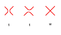
Figure 30: Interaction vertices in the $OSP(m|2n)$ symmetric sigma model on the square lattice.

A trivial rescaling of the partition function and isotropy of the model allows one to set the first two weights equal to $1$. The remaining weight is a free bare parameter. It was found in [7] that for any $w>0$ and $m-2n<2$ the lattice model is indeed described at large distance by the UV limit of the sigma model, ie a set of $m-1$ free uncompactified bosons and $n$ pairs of symplectic fermions, with a central charge $c=m-2n-1$. The value $w=0$ is critical, and was argued in [7, 15] to correspond to the critical point of the sigma model. Note that for $m-2n$ fixed, there exists a particular value of the crossing weight $w$ where the model is integrable, and coincides with the one in [12].

Of course, the geometrical representation of the invariant tensors allows for a full geometrical formulation of the model, that can then be extended to values of $m,n$ not integer. The model so obtained is made of loops covering every link of the lattice, and possibly self-intersecting once on the vertices, with a fugacity $m-2n$, and a weight $w$ per crossing. The continuum limit was found to be a naive extrapolation from the results at $m,n$ integer. Note that this model differs from the usual formulation of the $Q$-state critical Potts model with $m-2n\equiv\sqrt{Q}$ only in that crossings are allowed. This however changes the universality class deeply. For instance, all the $L$-leg operators which have non trivial, $Q$-dependent scaling dimensions in the Potts model for $-2\leq\sqrt{Q}\leq 2$, now have logarithmic correlators with vanishing effective dimension. This is because the symmetry being spontaneously broken the fundamental field has non vanishing expectation value, and thus the fields $\phi_{a}$ do exist in the conformal field theory, unlike in the case of a compact boson.

[Paths that can self intersect at a vertex but not at a bond are called trails in the literature, and “bond self avoiding models” by contrast with “site self avoiding”. The case $m-2n=0$ we consider below would correspond to “fully packed trails”. People have considered ordinary (dilute) trails which are in the same universality class as dilute SAW and trails at the theta point. Those have been shown to be in the same universality class as “growing self avoiding trails”, themselves a particular case of the trajectory of a particle moving on a lattice with random distribution of scattering rotators. See [16, 17]. In the context of such trajectories, it has been remarked already that when one dilutes the set of random rotators from maximum concentration $C_{L}=C_{R}=1/2$ (i.e., add intersections), the exponents change.]

5.2 Coupling constant and physical exponents of the $OSP(2|2)$ model

We now specialize to the case of interest here, the $OSP(2|2)$ model. The UV limit is easy to understand. We can parametrize the supersphere

$$(\phi_{1})^{2}+(\phi_{2})^{2}+2\psi_{1}\psi_{2}=1$$ (188)

by setting

$$\phi_{1} = \cos\phi\ (1-\psi_{1}\psi_{2})$$

$$\phi_{2} = \sin\phi\ (1-\psi_{1}\psi_{2}),\qquad\phi\equiv\phi+2\pi$$ (189)

The action then reads

$$S=\frac{1}{2g_{\sigma}}\int d^{2}x\left[(\partial_{\mu}\phi)^{2}(1-2\psi_{1}\psi_{2})+2\partial_{\mu}\psi_{1}\partial_{\mu}\psi_{2}-4\psi_{1}\psi_{2}\partial_{\mu}\psi_{1}\partial_{\mu}\psi_{2}\right]$$ (190)

The coupling $g_{\sigma}>0$ flows to zero at large distances. On the other hand, we can absorb it by rescaling all fields so the action reads

$$S=\frac{1}{2}\int d^{2}x\left[(\partial_{\mu}\phi)^{2}(1-2g_{\sigma}\psi_{1}\psi_{2})+2\partial_{\mu}\psi_{1}\partial_{\mu}\psi_{2}+4g_{\sigma}\psi_{1}\psi_{2}\partial_{\mu}\psi_{1}\partial_{\mu}\psi_{2}\right]$$ (191)

where now $\phi$ has a different radius, $\phi\equiv\phi+\frac{2\pi}{\sqrt{g_{\sigma}}}$. We see that as $g_{\sigma}\rightarrow 0$ all interaction terms disappear and we get a free boson $\phi$ together with a pair of free symplectic fermions $\psi_{1,2}$. Moreover the radius of compactification goes to infinity in that limit, so the boson $\phi$ appears as non compact.

This holds in the true large distance limit. At intermediate scales, we can use the RG equation for the coupling [18]

$$\frac{dg_{\sigma}}{d\log l}=\frac{m-2n-2}{2\pi}g_{\sigma}^{2}=-\frac{1}{\pi}g_{\sigma}^{2}$$ (192)

Writing more generally

$$\frac{dg_{\sigma}}{d\log l}=-\alpha g_{\sigma}^{2}$$ (193)

we see that $g_{\sigma}$ approaches its vanishing large distance value as

$$\frac{1}{g_{\sigma}}=\frac{1}{g_{\sigma}^{0}}+\alpha\log(l/l_{0})\simeq\alpha\log(l/l_{0})$$ (194)

Here, $l$ is a characteristic dimensionless scale ratio, roughly of the order of the ratio of the scale at which one is observing the physics to the lattice cut-off. On the cylinder, $l$ can be identified with the width in lattice units, $l=N$.

In the limit of large $l$, we can estimate more precisely the contribution to the spectrum coming from the boson $\phi$. Recall that for a free bosonic theory where the action is normalized as $S=\frac{1}{8\pi}\int(\partial_{\mu}X)^{2}$ and the field compactified as $X\equiv X+2\pi R$, the spectrum of dimensions [19] is

$$\Delta+\bar{\Delta}=\frac{e^{2}}{R^{2}}+\frac{m^{2}R^{2}}{4}$$ (195)

Matching the normalization gives $R^{2}=4\pi/g_{\sigma}$ in our case, and thus we expect the scaled gaps coming from the bosonic degrees of freedom to read, at large distances :

$$\Delta+\bar{\Delta}=\frac{e^{2}}{4\pi\alpha\log(l/l_{0})}+m^{2}\pi\alpha\log(l/l_{0})$$ (196)

In the limit $l\rightarrow\infty$ the dimensions become degenerate and the spectrum can be considered as a continuum starting above $\Delta+\bar{\Delta}=0$. To emphasize the latter point, consider the contribution to the partition function coming from the $\phi$ degrees of freedom. The system is defined on a torus of periods $l$ and $l^{\prime}$, with $l^{\prime}/l=\tau$. Denote $q=\exp(2i\pi\tau)$.

$$Z_{\phi} = \frac{1}{\eta\bar{\eta}}\sum_{e,m}q^{(e/R+mR/2)^{2}/2}\ \bar{q}^{(e/R-mR/2)^{2}/2}$$ (199)

$$= \frac{R}{\sqrt{2}}\frac{1}{\sqrt{\hbox{Im }\tau}\ \eta\bar{\eta}}\sum_{m,m^{\prime}}\exp\left(-\frac{\pi R^{2}|m\tau-m^{\prime}|^{2}}{2\ \hbox{Im }\tau}\right)$$

$$\begin{array}[]{c}\approx\\ R\rightarrow\infty\end{array} \frac{R}{\sqrt{2}}\frac{1}{\sqrt{\hbox{Im }\tau}\ \eta\bar{\eta}}$$

where $\eta=q^{1/24}\prod_{n=1}^{\infty}(1-q^{n})=q^{1/24}P(q)$. Observe now that one can write :

$$\frac{1}{\sqrt{\hbox{Im }\tau}\ \eta\bar{\eta}}=4\int_{0}^{\infty}\frac{q^{s^{2}}\bar{q}^{s^{2}}}{\eta\bar{\eta}}\ ds$$ (200)

which can be interpreted as an integral over a continuum of critical exponents $\Delta=\bar{\Delta}=s^{2}$. In the partition function (199), $R$ plays the role of the density of levels, and is proportional to the (diverging) size of the target space.

Going back to the specific case of the $OSP(2|2)/OSP(1|2)$ model, we set $\alpha=1/\pi$. We get the radius $R^{2}=4\log(l/l_{0})$, and the contribution of the free boson $\phi$ to the spectrum is :

$$\Delta+\bar{\Delta}=\frac{(e_{2})^{2}}{4\log(l/l_{0})}+(m_{2})^{2}\log(l/l_{0})$$ (201)

with $e_{2},m_{2}$ arbitrary integers. Suppose now we consider the sigma model with a combination of periodic and antiperiodic boundary conditions for the symplectic fermions. These get untwisted, and add to $Z_{\phi}$ the discrete spectrum of a free boson at the free fermion point, which is given by equation (195) with a radius $R^{2}=1$. The quantum numbers associated to the fermions will be denoted $e_{1},m_{1}$. Thus we expect :

$$\Delta+\bar{\Delta}={(e_{1})^{2}}+\frac{(m_{1})^{2}}{4}+\frac{(e_{2})^{2}}{4\log(l/l_{0})}+(m_{2})^{2}\log(l/l_{0})$$ (202)

We can now compare with formula (4.3.1). It is not entirely clear how constrained the quantum numbers might be in the lattice realization we are considering. But observe that finite scaled gaps occur for $m_{+}=m_{-}=m$ and converge to

$$x=\frac{m^{2}}{g}+\frac{1}{4}g(n_{+}+n_{-})^{2}+\frac{1}{4}K(\gamma,N)(n_{+}-n_{-})^{2}$$ (203)

When $\gamma$ tends to $\pi/2$, equations (158) and (171) give the coupling constants :

$$g=1\ ,\qquad K(\pi/2,N)\sim\frac{A^{\prime}}{\log N}$$ (204)

The numerical results are compatible with $A^{\prime}=1$. This suggests the identifications :

$$e_{1} = \frac{1}{2}(m_{+}+m_{-})=m$$

$$m_{1} = n_{+}+n_{-}$$

$$e_{2} = n_{+}-n_{-}$$

$$m_{2} = \frac{1}{2}(m_{+}-m_{-})=0$$

Note that the quantum numbers are (weakly) correlated : the integers $m_{1},e_{2}$ are such that $(m_{1}+e_{2})$ is even.

5.3 Interpretation of the staggered six-vertex model for $\gamma<\pi/2$

In preparation for the subsequent discussion, we will denote the effective (square) radius of the non compact boson by $(R_{2})^{2}$ (equal to $4\log(l/l_{0})$ for $\gamma=\pi/2$) and the radius of the compact boson by $(R_{1})^{2}$ (equal to $1$ for $\gamma=\pi/2$). Away from $\gamma=\pi/2$, it would be reasonable to try and interpret our results in terms of a deformation of the supersphere sigma model. Several scenarios are a priori possible. From the numerical results, the compact direction clearly has a modified radius which becomes :

$$(R_{1})^{2}=g=\frac{2\gamma}{\pi}$$ (205)

As for the non compact direction, a first possibility would be to consider a constant $\alpha(\gamma)$ in the foregoing discussion. Although it provides reasonable results, much better fits are obtained with a radius going like $\log(l/l_{0})$ for $\gamma\neq\pi/2$; specifically, we find :

$$(R_{2})^{2}=\frac{\pi-2\gamma}{5\gamma}[\log(l/l_{0})]^{2}$$ (206)

Note that this becomes ill-defined as $\gamma$ tends to $\pi/2$, where there is crossover to a behaviour linear in $\log(l/l_{0})$.

The most naive interpretation of the corresponding target space would be a torus with one period diverging like $\log(l/l_{0})$ in the scaling limit. This is reminiscent of results on the sausage model [20] which is a deformation of the usual sphere sigma model. There however, the theory instead of being massless in the IR is massless in the UV, while the target space in that limit is asymptotically a cigar. The dependence of the cigar dimensions on the RG scale and the anisotropy parameter are however reminiscent of ours; in particular the “long dimension” goes as the logarithm of the RG coordinate in both cases.

Another, more suggestive interpretation, can be obtained if we consider the partition function of our model on the torus. Set $\gamma=\pi/t$ so $(R_{2})^{2}=\frac{t-2}{5}[\log(l/l_{0})]^{2}$. Using the continuum representation (199) and reabsorbing the $t-2$ prefactor that comes from the dependence of $R_{2}$ upon $t$ into the continuously varying exponents we obtain the partition function :

$$Z\propto\frac{\log(l/l_{0})}{(\eta\bar{\eta})^{2}}\sum_{e,m=-\infty}^{\infty}\int_{0}^{\infty}ds\ q^{{s^{2}\over t-2}+{(m-te)^{2}\over 4t}}\ \bar{q}^{{s^{2}\over t-2}+{(m+te)^{2}\over 4t}}$$ (207)

where the proportionnality constant is a presumably non universal quantity, independent of $t$, equal appproximately to $1/\sqrt{10}$. Observe now that ${2(t+1)\over t-2}-{24\over 4(t-2)}=2$ so the conformal weights can be written as well, with respect to $c={2(t+1)\over t-2}$, as :

$$h={s^{2}+{1\over 4}\over t-2}+{(m\mp te)^{2}\over 4t}$$ (208)

This coincides with the contribution of the continuous representations to the spectrum of the Euclidian black hole CFT $SL(2,R)/U(1)$ coset model [21].

It might be useful here to give some quick reminders for the spectrum of this model. The central charge for level $k$ is :

$$c_{\rm BH}={2(k+1)\over k-2}$$ (209)

Normalizable operators come in two kinds. There is the ones (delta functions normalizable) associated with the principal continuous series $j=-{1\over 2}+is$ with conformal weight :

$$h=-{j(j+1)\over k-2}+{(n\pm kw)^{2}\over 4k}={s^{2}+{1\over 4}\over k-2}+{(n\pm kw)^{2}\over 4k}$$ (210)

and the ones coming from the discrete series. They have $j\in\left[{1-k\over 2},-{1\over 2}\right]$ together with rules relating allowed values to $w,n$. The net result is that these fields all have dimensions larger than the bottom of (210). Note that the identity field $h=0$ is not among the normalizable states, which is consistent with the fact that we do not observe (after the obvious identification $k\equiv t$) $c_{\rm BH}$ in the lattice model but $c_{\rm BH}-24{1\over 4(k-2)}=2$.

Of course the partition function of the Euclidian black hole theory should naively be infinite since it involves infinite dimensional representations of $SL(2)$. The introduction of a Liouville wall at finite distance in the target space [22] gives a density of states $\rho(s)\propto\log\epsilon$ to leading order, which agrees with our results provided we identify $\epsilon\equiv l/l_{0}$, and thus the size of the system (it would certainly be interesting to investigate the subleading behaviour, which depends on $s$, in the lattice data).

Finally, we note that in [22], the sum (4.17) implies some combinatorial contraints on the descendents, which we have not studied in the lattice model.

Note that further twisting and reduction of the vertex model gives rise to parafermionic theories, which are themselves cosets $SU(2)/U(1)$. It is not clear how this might be related to the identification of the untwisted vertex model with $SL(2,R)/U(1)$.

6 Geometrical interpretation of the critical exponents

For the $OSP(m|2n)$ models in their Goldstone phases, the continuous spectrum of critical exponents has its origin (like in the case of a pure non compact boson) in the existence of infinitely many operators with vanishing scaling dimension (the powers of $\phi$ in the case of the non compact boson), which in itself is a consequence of the spontaneously broken symmetry [7]. An obvious question is whether a similar interpretation exists for our model.

Some insight can be gained by considering the limit $\gamma\to\pi/2$ which is related to the $OSP(2|2)$ model. In the latter, exponents of the order parameter are related with geometrical correlations of the degrees of freedom carrying lines, and therefore it is tempting to ask whether this might hold away from the limit point as well. Before discussing this, it is important to notice that the staggered six-vertex model at $\gamma=\pi/2$ (and the equivalent 38-vertex model) with periodic boundary conditions correspond, strictly speaking, to the model of [7, 10] where the $OSP$ symmetry is broken by the boundary. This is the reason why the spectrum of conformal weights contains a compact boson with $(R_{1})^{2}=1$, and thus non trivial, finite exponents. Within the geometrical interpretation to be discussed below, this will correspond to the existence of some correlators having non trivial weights, while others do behave as in [7].

Let us now be more specific. As shown in section 2.3, summing on $2\times 2$ vertex blocks and choosing the right basis, the staggered six-vertex model is equivalent to the 38-vertex model. Any lattice configuration within this model is completely covered by polygons of three different types : oriented lines, bare thin lines and bare thick lines. The particular point $\gamma=\pi/2$, as well as our discussion on Goldstone phases, suggests to consider geometrical correlations associated with these lines.

6.1 Correlation functions with no thin or thick line

Consider first the watermelon correlation function (as illustrated on the figure 31) consisting of a forced even number $2r$ of positively-oriented lines (that is, we force $2r$ such lines to propagate through the system, on top of fluctuating numbers of positively and negatively oriented lies in equal number and bare lines). The critical exponent of this correlation function is given by the lowest-energy state in the sector with fixed total spin $S=2r$ and $C=1$. According to equation (4.3.1), this state is $\varphi_{(r,r),(0,0)}$. According to equation (105), this is an eigenstate of the operator $C$, with eigenvalue one.

6.2 Correlation functions with one thin or thick line

Consider the correlation function consisting of a forced odd number $2r-1$ of positively-oriented lines, along with one bare (thin or thick) line. The critical exponent of the correlation function with a thin (resp. thick) line is given by the lowest-energy state in the sector with fixed total spin $S=2r-1$ and $C=1$ (resp. $C=-1$). Both states $\varphi_{(r,r-1),(0,0)}^{\pm}$ have the physical exponent $x_{(r,r-1),(0,0)}$. Thus, the correlation functions with one thin or thick line have the same exponent $x_{(r,r-1),(0,0)}$.

6.3 Correlation functions with one thin line and one thick line

Consider the correlation function consisting of a forced even number $2r$ of positively-oriented lines, along with one thin line and one thick line. The critical exponent of this correlation function is given by the lowest-energy state in the sector with fixed total spin $S=2r$ and $C=-1$. This state is $\varphi_{(r+1,r-1),(0,0)}^{-}$, with physical exponent $x_{(r+1,r-1),(0,0)}$.

In the particular case $r=0$, this exponent becomes :

$$x_{(1,-1),(0,0)}=K(\gamma,N)$$ (211)

This exponent vanishes in the thermodynamic limit. So the two-leg correlation function consisting of one thin line and one thick line belongs to the continuous subspectrum associated to the ground state.

Figure 31: Some “watermelon” correlation functions. (a): no bare line, (b)-(c): one bare line, (d): one thin line and one thick line.

6.4 Interpretation

The physical interpretation we suggest for the continuum limit of the 38-vertex model is thus the following. The arrow degrees of freedom can be treated like the usual domain boundaries for a RSOS model which renormalizes, at large distances, to a compactified free bosonic field with radius $R_{1}$. A correlation function involving a certain number $S$ of positively oriented lines corresponds for this bosonic field to a magnetic or vortex operator, whose physical exponent is given by $x=gS^{2}/4$.

Meanwhile, correlators involving in addition thin and thick lines as well have, in the thermodynamic limit, exponents entirely determined from the contribution of the arrow degrees of freedom. Thin and thick lines correspond thus to operators with vanishing exponents and (presumably) logarithmic correlators, and behave similarly to the crossing lines in the models of [7].

7 Conclusion, open problems

First and foremost, we believe this work puts on firm ground the existence of a continuous spectrum of critical exponents in a model with a finite number of lattice degrees of freedom per site (link), justifying fully the conclusions of [7, 8] .

It is truly remarkable that a proper staggering of the simple six-vertex model could give rise to such interesting behaviour: obvious directions for future work are plenty, and include an analytic derivation of the coupling constant $K$, a better understanding of the relationship with $SL(2,R)/U(1)$, and of the effect of the various twist and truncations necessary to produce the Potts and RSOS versions of this model.

It should also be possible to generalize the problem to some higher spin version. Some comments on Bethe equations are in order here. Recall that the usual source term for these equations reads, in the case of spin $1/2$ :

$$\left({\sinh{1\over 2}(\alpha-i\gamma)\over\sinh{1\over 2}(\alpha+i\gamma)}\right)^{N}$$ (212)

One might think of changing it through real heterogeneities $\pm\Lambda$, leading to equations which have been used a great deal in the study of massive deformations [23] :

$$\left({\sinh{1\over 2}(\alpha-\Lambda-i\gamma)\over\sinh{1\over 2}(\alpha-\Lambda+i\gamma)}\right)^{N/2}\left({\sinh{1\over 2}(\alpha+\Lambda-i\gamma)\over\sinh{1\over 2}(\alpha+\Lambda+i\gamma)}\right)^{N/2}$$ (213)

One could also think of changing it through imaginary heterogeneities. The simplest case would correspond to adding “string heterogeneities”, i.e., for the simplest case of the two string, formally $\Lambda=i\gamma$. Clearly however half the modified source terms cancel out, leaving :

$$\left({\sinh{1\over 2}(\alpha-2i\gamma)\over\sinh{1\over 2}(\alpha+2i\gamma)}\right)^{N}$$ (214)

which is nothing but the source term for a spin one chain. In general, heterogeneities of the type p-string will lead to the equations for the spin $p/2$ chain. The other natural possibility would be to add heterogeneities of the anti-string type, ie $\Lambda=i\pi$. Up to a shift $\alpha\rightarrow\alpha+i\pi$, this produces however the initial equations, and is well known to simply change the Hamiltonian from ferromagnetic to antiferromagnetic. The possibility we encountered in this paper consists in adding heterogeneitiesright in the middle of the “physical strip”, at $\Lambda=i{\pi/2}$. Note that the higher spin generalization is obvious by changing $i\gamma$ to $2si\gamma$ everywhere.

It is also fascinating that the model should interpolate between $OSP(2/2)$ and $SO(4)$ symmetries when $\gamma$ goes from $\pi/2$ to zero. This suggests the existence of a possible quantum group symmetry all along the line, which we have unfortunately not yet been able to identify.

References

• [1] R.J. Baxter, Proc. R. Soc. Lond. A 383, 43 (1982).
• [2] V. Schomerus, Phys. Rep. 431, 29 (2006).
• [3] J. Maldacena and H. Ooguri, J. Math. Phys. 42, 2929 (2001).
• [4] M. R. Zirnbauer, Conformal field theory of the integer quantum Hall plateau transition, hep-th/9905054.
• [5] B. Duplantier, Phys. Rep. 184, 229 (1989).
• [6] A.V. Belitsky, S.E. Derchakov, G.P. Korchemsky and A.N. Manashov, Baxter Q-operator for graded SL($2|1$) spin chain, hep-th/0610332.
• [7] J.L. Jacobsen, N. Read and H. Saleur, Phys. Rev. Lett. 90, 090601 (2003).
• [8] F. Essler, H. Frahm and H. Saleur, Nucl. Phys. B 712, 513 (2005).
• [9] J.L. Jacobsen and H. Saleur, Nucl. Phys. B 743, 207 (2006).
• [10] J.L. Jacobsen and H. Saleur, Nucl. Phys. B 716, 439 (2005).
• [11] R.J. Baxter, Studies in Appl. Math. 50, 51 (1971).
• [12] M. J. Martins, B. Nienhuis and R. Reitman, Phys. Rev. Lett. 81, 504 (1998).
• [13] W. H. Press, S. A. Teukolsky, W. T. Vetterling and B. P. Flannery, Numerical Recipes in C, 2nd edition (Cambridge University Press, 1992).
• [14] F.C. Alcaraz, M.N. Barber and M.T. Batchelor, Ann. Phys. 182, 280 (1988).
• [15] N. Read and H. Saleur, Nucl. Phys. B 613, 409 (2001).
• [16] A.I. Owczarek and T. Prellberg, J. Stat. Phys. 79, 951 (1995).
• [17] M.S. Cao and E.G.D. Cohen, J. Stat. Phys. 87, 147 (1997).
• [18] E. Abdalla, M.C.B.Abdalla and K.D. Rothe, Non-perturbative methods in two-dimensional quantum field theory (World Scientific, 1991).
• [19] P. Di Francesco, P. Mathieu and D. Senechal, Conformal field theory (Springer-Verlag, New York, 1997).
• [20] V. Fateev, E. Onofri and A.B. Zamolodchikov, Nucl. Phys. B 406, 521 (1993).
• [21] R. Dijkgraaf, H. Verlinde and E. Verlinde, Nucl. Phys. B 371, 269 (1992).
• [22] A. Hanany, N. Prezas and J. Troost, JHEP 04, 014 (2002).
• [23] See for instance: C. Destri and H. de Vega, Nucl. Phys. B 438, 413 (1995); N. Yu Reshetikhin and H. Saleur, Nucl. Phys. B 419, 507 (1994).