Strongly correlated fermions after a quantum quench

Abstract

Using the adaptive time-dependent density-matrix renormalization group method, we study the time evolution of strongly correlated spinless fermions on a one-dimensional lattice after a sudden change of the interaction strength. For certain parameter values, two different initial states (e.g., metallic and insulating), lead to observables which become indistinguishable after relaxation. We find that the resulting quasi-stationary state is non-thermal. This result holds for both integrable and non-integrable variants of the system.

Recent experiments on optical lattices have made it possible to investigate the behavior of strongly correlated quantum systems after they have been quenched. In these experiments, the system is prepared in an initial state $|\psi_{0}\rangle$ and then is pushed out of equilibrium by suddenly changing one of the parameters. Prominent examples are the collapse and revival of a Bose-Einstein condensate (BEC) Nature:Bloch , the realization of a quantum version of Newton’s cradle Nature:Weiss , and the quenching of a ferromagnetic spinor BEC Nature:Sadler . All of these systems can be considered to be closed, i.e., have no significant exchange of energy with a heat bath, so that energy is conserved to a very good approximation during the time evolution. Furthermore, since these systems are characterized by a large number of interacting degrees of freedom, application of the ergodic hypothesis leads to the expectation that the time average of observables should become equal to thermal averages after sufficiently long times. Various authors have recently given voice to such an expectation sengupta:053616 ; berges:142002 ; corinna:quench . However, the experiment on one dimensional (1D) interacting bosons shows no thermalization, a behavior that was ascribed to integrability Nature:Weiss . Rigol et al. found that an integrable system of hard-core bosons relaxes to a state well-described by a Gibbs ensemble that takes into account the full set of constants of motion marcos:relax ; similar results were found for the integrable Luttinger model cazalilla:156403 .

For a closed system, the set of expectation values of all powers of the Hamiltonian $\hat{H}$ constitute an infinite number of constants of motion, irrespective of its integrability. Therefore, the question of the importance of integrability in a closed system that is quenched arises. We address this issue by investigating the full time evolution of a strongly correlated system whose integrability can be easily destroyed by turning on an additional interaction term. We show, using the recently developed adaptive time-dependent density matrix renormalization group method (t-DMRG) Uli_timeevolve ; white:076401 ; luo:049701 ; schmitteckert:121302 ; manmana:269 , that, in a certain parameter range, two different initial states with the same energy relax, to within numerical precision, to states with indistinguishable momentum distribution functions. A comparison with quantum Monte Carlo (QMC) simulations shows, however, that they do not correspond to a thermal state. By using a generalized Gibbs ensemble balian ; marcos:relax ; cazalilla:156403 ; marcos:relax2 with the expectation value of the powers of the Hamiltonian $\langle{\hat{H}}^{n}\rangle$ as constraints, we can improve the agreement with the time averages of the evolved system. This applies to both the integrable as well as the non-integrable case.

In this Letter, we investigate the Hamiltonian

$$\hat{H}=-t_{\rm h}\sum_{j}\left(c_{j+1}^{\dagger}c_{j}^{\phantom{\dagger}}+h.c.\right)+V\sum_{j}n_{j}^{\phantom{\dagger}}n_{j+1}^{\phantom{\dagger}}\;,$$ (1)

with nearest-neighbor hopping amplitude $t_{\rm h}$ and nearest-neighbor interaction strength $V$ at half-filling. The $c_{i}^{\left(\dagger\right)}$ annihilate (create) fermions on lattice site $i$, $n_{i}=c_{i}^{\dagger}c_{i}^{\phantom{\dagger}}$, and we take $\hbar=1$. We measure energies in units of $t_{\rm h}$, and, accordingly, time. The well-known ground-state phase diagram for the half-filled system consists of a Luttinger liquid (LL) for $V<V_{c}=2$, separated from a charge-density-wave (CDW) insulator ($V>V_{c}$) by a quantum critical point $V_{c}$ spinless_fermions . This model is integrable, with an exact solution via the Bethe ansatz HBenergy . We consider open chains of up to $L=100$ sites pushed out of equilibrium by suddenly quenching the strength of $V$ from an initial value $V(t=0)=V_{0}$ to a different value $V(t>0)=V$. Furthermore, we study the effect of adding a next-nearest-neighbor repulsion $V_{2}\sum_{j}n_{j}^{\phantom{\dagger}}n_{j+2}^{\phantom{\dagger}}$ to the model, which makes it non-integrable. We compute the time evolution using the Lanczos time-evolution method lubich_timeevolve ; manmana:269 ; noack:93 ; ED_review and the adaptive t-DMRG. We study the momentum distribution function (MDF) $\langle n_{k}\rangle(t)=\frac{1}{L}\sum_{l,m=1}^{L}e^{ik(l-m)}\langle c^{\dagger}_{l}c_{m}\rangle(t),$ i.e., the Fourier transform of the one-particle density matrix, $\rho_{lm}=\langle c^{\dagger}_{l}c_{m}\rangle$. In the t-DMRG, we utilize the Trotter approach developed in Refs.  Uli_timeevolve ; white:076401 as well as the Lanczos approach schmitteckert:121302 ; manmana:269 with additional intermediate time steps added within each time interval feiguin:020404 . We hold the discarded weight fixed to $\varepsilon\leq 10^{-9}$ during the time evolution, but additionally restrict the number of states kept to be in the range $100\leq m\leq 1500$. In all calculations presented here, the maximum error in the energy, which is a constant of motion, is 1%, and, in most cases, less than 0.1%, at the largest times reached.

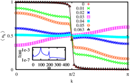
Figure 1: (color online) Time evolution of an initial LL state ($V_{0}=0.5$) in the strong coupling limit with $V=100$ for $L=100$ sites at the times indicated. Inset: spectral analysis of $\langle n_{\pi}(t)\rangle$.

When an initial LL state is quenched to the strong-coupling regime, $V\gg t_{\rm h}$, we find that $\langle n_{k}(t)\rangle$ (Fig. 1), exhibits collapse and revival on short time scales, whereas the density-density correlation function remains essentially unchanged, i.e., retains the power-law decay of the LL. This can be understood by considering a quench to the atomic limit, $t_{\rm h}=0$. In this limit, all observables that commute with the density operator, including the density-density correlation function, are time-independent. Furthermore, since the only remaining interaction is the nearest-neighbor density-density interaction, it can be shown analytically that the one-particle density matrix $\rho_{m\,l}(t)$ involves only two frequencies ($\omega_{1}=V$ and $\omega_{2}=2V$), resulting in a periodic oscillation with a revival time of $T_{\rm revival}=2\pi/V$ UnpublishedSalva . Thus, in analogy to the observed collapse and revival of a BEC in an optical lattice Nature:Bloch , the single-particle properties of an initial LL state exhibit collapse and revival with this period. For the strong-coupling regime, the time evolution retains the oscillatory behavior of the atomic limit; two frequencies $\omega_{1}$ and $\omega_{2}$ are indeed dominant in the spectrum, as can be seen in the inset of Fig. 1. However, the finite hopping amplitude leads to a dephasing of the oscillation on a time scale of $t_{\rm dephase}\sim 1/t_{h}$.

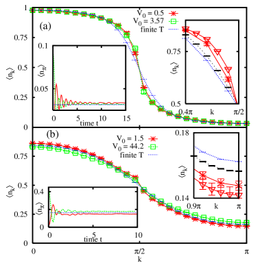
Figure 2: (color online) Time-averaged momentum distributions when quenching (a) from $V_{0}=0.5$ to $V=2$ (quantum critical point) and (b) from $V_{0}=1.5$ to $V=5$ (insulator) for $L=50$ sites. The time averages of two independent initial states with the same energy are compared to each other and to the thermal expectation value. In the right inset, results for $L=50$ ($\ast$) are compared to $L=100$ ($\bigtriangledown$) for the regions with the largest differences. As a reference, finite $T$ data for $L=50$ (dotted line) and $L=100$ (dashed line) are shown. Left insets: $\langle n_{\pi}\rangle$ vs. time t; the horizontal line is the finite $T$ value.

Afterwards, observables oscillate with a small amplitude around a fixed value, suggesting that the system reaches a quasi-stationary state. In order to further characterize such states, we study the evolution of the system for various values of $V$ up to times one order of magnitude larger than $1/t_{h}$ when applying the t-DMRG and up to two orders of magnitude larger when using full diagonalization (FD). We find that the time averages for the longer times reachable by the FD agree with the time averages for the times reachable by the t-DMRG. Therefore, we conclude that the relevant time scale for the relaxation is indeed given by $1/t_{h}$. In Fig. 2, the MDFs, obtained by performing an average in time from time $t=3$ to $t=10$ at the quantum critical point, $V=V_{c}$, and at a point in the CDW region, $V=5$, are shown. In order to investigate to what extent the (quasi-)stationary behavior is generic, we examine its dependence on the initial state. We do this by preparing two qualitatively different initial states with the same average energy $\langle\hat{H}\rangle$ for each case: one a ground state in the LL regime and the other a ground state in the CDW regime. This is possible for a certain range of $V$ in the intermediate coupling regime. In Fig. 2, results for two such initial states are compared with each other and with the MDF obtained for a system in thermal equilibrium and the same average energy, calculated using QMC simulations QMC .

At the critical point, $V=V_{c}$, Fig. 2(a), the MDFs for the two initial states coincide with each other, to within the accuracy of the calculations (approximately the symbol size) or less. Therefore, information about the initial state is not preserved in this quantity, consistent with the expectation for an ergodic evolution. However, the difference from the thermal distribution is significant; thermalization is not attained. The left inset shows the time evolution of $\langle n_{k}\rangle(t)$ for $k=\pi$ for both initial conditions, demonstrating that the system reaches a quasi-stationary state. A small, but discernible shift from the thermal value (horizontal line) can also be seen for both initial conditions, even at $k=\pi$. In the right inset, the points with the largest differences just below the Fermi vector $k_{F}=\pi/2$ are plotted when the system size is doubled from $L=50$ to $L=100$. An analysis of the data for $L=100$ does not alter our conclusion.

In order to investigate the importance of quantum criticality, we have also examined the behavior for $V=1.5$ and $V=2.5$ (not shown), i.e., below and above the transition point. We find almost identical behavior, indicating that the lack of thermalization is not associated with the quantum critical point. Note, however, that the LL regime ($V<2$) is, in a sense, generically critical.

Figure 3: (color online) Time-averaged momentum distribution $\langle n_{k}\rangle$ for V=10. Inset: $\langle n_{\pi}\rangle$ vs. time $t$; the horizontal line is the finite-$T$ value.

For $V=5$, Fig. 2 (b), all three curves show small, but significant differences. This means that the time evolution starting from different initial states can be distinguished from each other as well as from the thermal state, i.e., neither relaxation to one distinguished quasi-stationary state nor thermalization occurs. For this case, $\mid V_{0}-V\mid$ is larger than for $V=2$, and, in addition, the values of $V_{0}$ necessary to obtain the same energy in the initial state ($V_{0}=1.5$ and $V_{0}=44.2165$) differ strongly. This suggests that the initial states are far apart from each other in some sense, a notion that will be made more precise below.

The differences with the thermal distribution increase for larger $\mid V_{0}-V\mid$. As can be seen in Fig. 3 for $V=10$, the difference between the time average and the thermal distribution is significant, clearly confirming that thermalization does not occur. The differences observed increase gradually as a function of $\mid V_{0}-V\mid$, ruling out a transition as suggested for the Bose-Hubbard model corinna:quench .

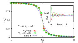
Figure 4: (color online) Comparison of QMC and time-averaged values of the momentum distribution $\langle n_{k}\rangle$ for the non-integrable case with $V=2$ and $V_{2}=0.4$. Inset: the same as in Fig. 3.

In order to investigate the impact of the lack of integrability on thermalization, we now extend our model (1) by turning on a next-nearest-neighbor interaction. In Fig. 4, we display results with $V_{0}=0.5$ and $V_{0}=2.46689$ (zero n.n.n. interaction), and the quenched evolution at $V=2$, $V_{2}=0.4$. As in the integrable case, both initial states lead to indistinguishable time-averaged MDFs, but ones that are significantly different from the thermal one, showing differences very similar to those in Fig. 2(a). When $V_{0}=0.5$ and $V=10,\,V_{2}=1$ (not shown) the difference from the thermal state is comparable to the case shown in Fig. 3. Therefore, the non-thermal nature of the emerging steady state is clearly not related to the integrability of the system.

In order to shed light on the numerical results presented above and to characterize the quasi-stationary state, we consider a generalized ensemble in which the expectation values of higher moments of $\hat{H}$, which are constants of the motion, are taken as constraints. Note that the usual thermal density matrix $\hat{\varrho}_{\beta}$ is uniquely fixed by the single constraint $\langle\hat{H}\rangle_{\beta}=\langle\hat{H}\rangle$. Rigol et al. marcos:relax , find a generalized Gibbs ensemble, in which the density matrix is determined by maximizing the entropy taking into account the constraints, to be an appropriate choice marcos:relax ; balian ; marcos:relax2 . The general form of the statistical operator is then $\hat{\varrho}=\exp\left[-\sum_{n}\lambda_{n}\hat{O}_{n}\right],$ where the operators $\hat{O}_{n}$ form a set of observables whose expectation values remain constant in time. The values of the $\lambda_{n}$ are fixed by the condition that ${\rm Tr}\left(\hat{\varrho}\,\hat{O}_{n}\right)=\langle\hat{O}_{n}\rangle$, with $\hat{O}_{0}=1$ to enforce normalization. In some special cases like hard-core bosons in one dimension marcos:relax ; marcos:relax2 or the Luttinger model cazalilla:156403 , constants of motion can be found in terms of operators in second quantization. However, this is not possible for Bethe-ansatz-integrable systems. For any closed system, however, the quantities $\hat{O}_{n}={\hat{H}}^{n}$ can be used. Taking all powers as constraints would unambiguously fix all correlation functions to all lengths. For a finite system, it can be shown that $\hat{\varrho}$ is fully determined by $\text{dim}(\hat{H})$ powers of $\hat{H}$ UnpublishedSalva , for $\hat{H}$ with a bounded spectrum. The statistical expectation value of any observable is then given by ${\rm Tr}\left(\hat{\varrho}\>\hat{O}\right)=\sum\limits_{\nu}|\langle\nu|\psi_{0}\rangle|^{2}\langle\nu|\hat{O}|\nu\rangle$ (for a non-degenerate spectrum), where $|\psi_{0}\rangle$ is the initial state and $|\nu\rangle$ are the eigenstates of $\hat{H}$. It can be easily seen, that the r.h.s. of this expression equals the time average of $\langle\hat{O}\rangle(t)$.

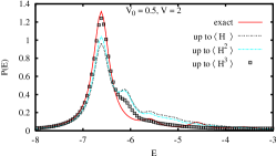
Figure 5: (color online) Influence of the constraints $\langle\hat{H}^{n}\rangle$ on the energy distribution function $P(E)$.

We now investigate the extent to which the statistical expectation value within the generalized Gibbs ensemble approaches the time average of the evolution after a quench by studying the energy distribution for a given state $|\psi\rangle$, defined as $P_{\psi}(E)=\sum_{\nu}\delta\left(E-\epsilon_{\nu}\right)|\langle\nu|\psi\rangle|^{2}$, which is normalized if $\langle\psi|\psi\rangle=1$. The energy distribution in the generalized Gibbs ensemble can analogously be defined as $P_{G}(E)={\rm Tr}\,\delta\left(E-\hat{H}\right)\hat{\varrho}$, with $\hat{\varrho}$ as defined previously. In Fig. 5, we show $P_{\psi}(E)$ calculated using full diagonalization on $L=16$ sites for an initial state $V_{0}=0.5$ evolved at the quantum critical point, $V=2$ compared with the distribution in the Gibbs ensemble $P_{G}(E)$ as the number of constraints is increased from 1 to 3. It is evident that increasing the number of constraints systematically improves the agreement and that only a small number of moments are necessary to obtain very good agreement.

The distance between two distributions can be estimated using the moments of the absolute differences, $\Delta_{n}=\int{\rm d}E\,E^{n}\,\mid P(E)-P^{\prime}(E)\mid\,$. Taking $\Delta_{0}/W$, with $W$ the bandwidth of $\hat{H}$, as an estimate of $\mid P(E)-P^{\prime}(E)\mid$, we see that the difference between moments of $\hat{H}$ for two different energy distributions $P$ and $P^{\prime}$ can be estimated as

$$\langle{\hat{H}}^{n}\rangle_{P}-\langle{\hat{H}}^{n}\rangle_{P^{\prime}}\leq\Delta_{n}\simeq\frac{1}{n+1}W^{n}\Delta_{0}\;.$$ (2)

Therefore, if the distance between the distributions $\Delta_{0}\ll 1$, then the relative difference of the moments $\left(\langle{\hat{H}}^{n}\rangle_{P}-\langle{\hat{H}}^{n}\rangle_{P^{\prime}}\right)/W^{n}<\Delta_{0}/(n+1)$ will also remain small, and observables will converge to values close to each other after a quench. For the cases of evolution with metallic and insulating initial states discussed above, we obtain $\Delta_{0}=0.12439$ for $V_{0}=0.5$ and $V_{0}=3.57463$ ($V=2$), and $\Delta_{0}=0.41521$ for $V_{0}=1.5$ and $V_{0}=44.2165$ ($V=5$). On the other hand, comparison of $P_{\psi}$ with the thermal distribution $P_{\beta}$ yields $\Delta_{0}=0.68581$ ($V_{0}=0.5$, $V=2$), and $\Delta_{0}=1.24616$ ($V_{0}=1.5$, $V=5$), respectively. Thus, the distance between the thermal distribution and the one defined by the initial states is always larger than those defined by the pair of initial states with the same energy, supporting our observation that thermalization does not occur.

In summary, our adaptive time-dependent density-matrix renormalization group simulations of the time evolution of a system of correlated spinless fermions after a quantum quench have exhibited the following generic behavior: Independently of its integrability or criticality, the system relaxes to a non-thermal quasi-stationary state. Observables relax to the same value when different initial states have the same energy and are sufficiently close to each other, i.e., the memory of the initial state is lost in the observables after relaxation. ‘Closeness’ can be quantified using a measure $\Delta_{0}$ which is based on the energy distributions defined for the initial state or for a given density matrix. Increasing the number of constraints (moments of $\hat{H}$) in a generalized Gibbs ensemble leads to convergence to the energy distribution defined by the initial state.

We acknowledge useful discussions with M. Arikawa, F. Gebhard, C. Kollath, S.R. White, and especially M. Rigol. S.R.M. acknowledges financial support by SFB 382 and SFB/TR 21. We acknowledge HLRS Stuttgart and NIC Jülich for allocation of CPU Time.

References

- (1) M. Greiner, O. Mandel, T. W. Hänsch, and I. Bloch, Nature 419, 51 (2002).
- (2) T. Kinoshita, T. Wenger, and D. S. Weiss, Nature 440, 900 (2006).
- (3) L. E. Sadler, J. M. Higbie, S. R. Leslie, M. Vengalattore, and D. M. Stamper-Kurn, Nature 443, 312 (2006).
- (4) K. Sengupta, S. Powell, and S. Sachdev, Phys. Rev. A 69, 053616 (2004).
- (5) J. Berges, S. Borsanyi, and C. Wetterich, Phys. Rev. Lett. 93, 142002 (2004).
- (6) C. Kollath, A. Läuchli, and E. Altman, unpublished, cond-mat/0607235.
- (7) M. Rigol, V. Dunjko, V. Yurovsky, and M. Olshanii, Phys. Rev. Lett. 98, 050405 (2007).
- (8) M. A. Cazalilla, Phys. Rev. Lett. 97, 156403 (2006).
- (9) A. J. Daley, C. Kollath, U. Schollwöck, and G. Vidal, J. Stat. Mech.: Theor. Exp., P04005 (2004).
- (10) S. R. White and A. E. Feiguin, Phys. Rev. Lett. 93, 076401 (2004).
- (11) H. G. Luo, T. Xiang, and X. Q. Wang, Phys. Rev. Lett. 91, 049701 (2003).
- (12) P. Schmitteckert, Phys. Rev. B 70, 121302(R) (2004).
- (13) S. R. Manmana, A. Muramatsu, and R. M. Noack, AIP Conf. Proc. 789, 269 (2005).
- (14) R. Balian, From Microphysics to Macrophysics: Methods and Applications of Statistical Physics, Texts and Monographs in Physics, Springer, 1991.
- (15) M. Rigol, A. Muramatsu, and M. Olshanii, Phys. Rev. A, 74, 053616 (2006).
- (16) J. Gubernatis, D. Scalapino, R. Sugar, and W. Toussaint, Phys. Rev. B 32, 103 (1985).
- (17) C. N. Yang and C. P. Yang, Phys. Rev. 150, 321 (1966).
- (18) M. Hochbruck and C. Lubich, BIT 39, pp. 620 (1999).
- (19) R. M. Noack and S. R. Manmana, AIP Conf. Proc. 789, 93 (2005).
- (20) N. Laflorencie and D. Poilblanc, Lect. Notes Phys. 645, 227 (2004).
- (21) A. E. Feiguin and S. R. White, Phys. Rev. B 72, 020404(R) (2005).
- (22) S. R. Manmana, S. Wessel, R. M. Noack, and A. Muramatsu, in preparation.
- (23) A. W. Sandvik, Phys. Rev. B 59, R14157 (1999).