Non-equilibrium work fluctuations for oscillators in non-Markovian baths

Abstract

We study work fluctuation theorems for oscillators in non-Markovian heat baths. By calculating the work distribution function for a harmonic oscillator with motion described by the generalized Langevin equation, the Jarzynski equality (JE), transient fluctuation theorem (TFT), and Crooks’ theorem (CT) are shown to be exact. In addition to this derivation, numerical simulations of anharmonic oscillators indicate that the validity of these nonequilibrium theorems do not depend on the memory of the bath. We find that the JE and the CT are valid under many oscillator potentials and driving forces whereas the TFT fails when the driving force is asymmetric in time and the potential is asymmetric in position.

I Introduction

Fluctuation theorems (FTs) which describe properties of the distribution of various nonequilibrium quantities, such as work and entropy, have been developed over the past decade phystod ; dynsys ; cohen ; jarzynski ; jarzynski2 ; crooks ; ND . Unlike most other relations in nonequilibrium statistical mechanics, remarkably, the FTs are applicable to systems driven arbitrarily far from equilibrium.

In particular, consider a classical finite-sized system in contact with a heat bath at temperature $T$ and driven by some generalized force $\lambda$ (e.g., volume, magnetic field). In equilibrium, the phase space distribution of the system is described by a well-defined statistical mechanical ensemble. The free energy $F$ can, in principle, be calculated and is a function of these parameters, i.e. $F=F(T,\lambda)$. At some time $t$, say $t=0$, $\lambda$ is varied via a fixed path $\lambda(t)$ to a later time $t=\tau$. If this process is carried out reversibly, the work done $W$ is simply the free energy difference $\Delta F=F(T,\lambda_{\tau})-F(T,\lambda_{0})$. More generically, the process is irreversible and the second law gives the well-known inequality

$$W\geq\Delta F.$$ (1)

An ensemble of such processes would yield the work probability distribution $P(W)$. The finite width of $P(W)$ is due to two stochastic sources: (1) The system configuration when the force is first initiated at $t=0$ is drawn from the equilibrium ensemble and (2) the path the system travels (in phase space) during the driving process is not deterministic due to the coupling with the heat bath. We study $P(W)$ in the light of three closely related theorems described below, the Jarzynski equality (JE) jarzynski , the transient fluctuation theorem (TFT) crooks ; ND ; dynsys , and Crooks’ theorem (CT) crooks ; ND .

The powerful nonequilibrium work relation due to Jarzynksi jarzynski allows one to exactly obtain equilibrium information (the free energy difference) from measurements of nonequilibrium processes. The JE states

$$<e^{-\beta W}>=e^{-\beta\Delta F},$$ (2)

where $\beta$ is the inverse temperature (with Boltzmann’s constant set to unity) and the average is over the distribution function $P(W)$ described above. The equality allows for the computation of $\Delta F$ even when the driving process is not adiabatic. This is to be compared with the inequality of Eq.(1). The JE has been shown for Hamiltonian systems jarzynski and Markovian stochastic systems jarzynski2 ; crooks ; ND .

Fluctuation theorems have been found for a wide class of systems and various nonequilibrium quantities, including work, heat, and entropy production. They are also generally divided into steady state cohen and transient theorems crooks ; ND ; dynsys . In this paper, we restrict our discussion to the transient fluctuation theorem for the mechanical work done. The TFT relates the ratio of probability distributions for the production of positive work to the production of negative work,

$$\frac{P(+W)}{P(-W)}=e^{+\beta W}.$$ (3)

Similar to the JE, the TFT has been derived in driven deterministic systems dynsys , and Markovian stochastic systems crooks ; ND ; markov1 ; markov2 ; markov3 .

Crooks crooks connected the JE and the TFT by using a relation very similar to Eq.(3), which we refer to as the Crooks’ theorem,

$$\frac{P_{F}(+W)}{P_{R}(-W)}=e^{+\beta W},$$ (4)

where $P_{F}(+W)$ is the probability distribution for work done as described in the above scenario and $P_{R}(-W)$ is the probability distribution for negative work done in a time-reversed driving process. The similarity between Eq.(3) and Eq.(4) is evident and the two theorems are, in fact, equivalent for a large class of systems. However, under certain asymmetries in the potential and the driving force, differences between the TFT and CT arise. In Sec. IV, we show one such scenario.

Unlike some other nonequilibrium quantities (e.g. heat and entropy), the classical mechanical work is an easily defined quantity, $W=\int_{0}^{\tau}dtf(t)\dot{x}(t)$. The original formulation of the JE jarzynski , however, relies on the generalized work, $W_{J}=-\int_{0}^{\tau}dt\dot{f}(t)x(t)$. As discussed in Refs. ND ; polymer , these two differ by the boundary conditions $f(\tau)x(\tau)-f(0)x(0)$ and care must be taken in defining the work in the fluctuation theorems.

The (space and time) extensiveness of $W$ (or $W_{J}$) demonstrates that second law “violations” become exponentially unlikely for thermodynamic systems; these violations only become observably probable for microscopic systems. Beyond purely theoretical interests, the recent investigations of molecular motors and nano-mechanical devices demonstrate the practical importance for understanding these universal nonequilibrium theorems, especially under increasingly realistic scenarios. Technological accessibility of microscopic systems has opened up experimental study and verification of the above theorems in various systems experiment ; liphardt .

In this paper, we focus on the JE, TFT, and CT for single harmonic and anharmonic oscillators. Using second order Langevin dynamics of a single oscillator, the work fluctuation theorems have been studied in Ref. harmonic . The work distribution function in harmonic polymer chains has been studied by one of us polymer . Both these papers and the derivations of the FTs for stochastic systems crooks ; ND ; markov1 ; markov2 ; markov3 utilize Markovian dynamics. Here, we study the FTs for oscillators coupled to non-Markovian baths. This extension is motivated by the intuition that there must be some memory to real heat baths and that all realistic models of heat baths, either classical classicbath or quantum mechanical quantumbath , are non-Markovian. Through analytic expressions for the harmonic oscillator and numerical simulations of anharmonic oscillators, we demonstrate that the memory of the bath does not affect the validity of the FTs.

In the next section, we briefly describe the model and the generalized Langevin dynamics. Sec. III contains explicit derivations of the JE, TFT, and CT in the harmonic limit where analytic calculations are possible. We show numerical results for the nonlinear oscillators in Sec. IV and summarize our results in the last section.

II the Model

We model the system as a unit mass particle in a one-dimensional potential with dynamics governed by the generalized Langevin equation genlangevin ,

$$\ddot{x}(t)=-\frac{dV(x)}{dx}+f(t)-\int_{0}^{t}dt^{\prime}\gamma(t-t^{\prime})\dot{x}(t^{\prime})+\eta(t),$$ (5)

where $V(x)$ is a conservative oscillator potential and$f(t)$ is an externally determined time-dependent driving force. The $\eta(t)$ and $\gamma(t)$ terms represent Gaussian noise and damping, respectively, and must be related through the fluctuation-dissipation theorem,

$$<\eta(t)>=0,\qquad<\eta(t)\eta(t^{\prime})>=T\gamma(t-t^{\prime}),$$ (6)

where $T$ is the temperature of the bath. In the white Gaussian noise limit, $\gamma(t)$ is proportional to a Dirac $\delta$-function and the more familiar “Markovian” Langevin equation is recovered. We mention that the damping is even in time $\gamma(t)=\gamma(-t)$, an important property to be used in the next section.

We use a potential $V(x)$ of the form

$$V(x)=\frac{\omega_{o}^{2}x^{2}}{2}+\frac{k_{3}x^{3}}{3}+\frac{k_{4}x^{4}}{4}$$ (7)

which can represent a truncation of the Taylor expansion of some complicated potential. We restrict ourselves to bounded potentials. $x$ can represent the spatial position, an angular variable as in Ref. harmonic , or a generalized coordinate. From this potential and the driving force $f(t)$ conjugate to $x$, the Hamiltonian $\mathcal{H}$ is clearly $\mathcal{H}(t)=\dot{x}^{2}/2+V(x)-f(t)x$. If the force is time-independent, the system would eventually reach equilibrium and the free energy $F$ can be simply calculated by $F=-Tln(\mathcal{Z})$, where $\mathcal{Z}$ is the partition function. In this ensemble, we recall that the Jarzynski work $W_{J}$ is not generally equal to the real mechanical work $W$ ND ; polymer . In the next section, we derive the work distribution function for the harmonic oscillator, i.e. $k_{3}=k_{4}=0$.

III The Harmonic Oscillator

At low temperatures, many potentials can be well approximated by the harmonic potential. Harmonic oscillators also have the practical virtue that a formal solution to Eq.(5) exists. We use this formal solution to derive the distribution functions for the Jarzynski generalized work $W_{J}$ and the real mechanical work $W$. The work distribution functions are then used to verify the JE and the TFT. (The TFT and CT are equivalent for the harmonic oscillator.) The analytic expressions in this section are analogous to the expressions from Ref. polymer with three main differences. The primary difference is that the noise is colored here. Second, we use the full second order Langevin equation instead of taking the strongly overdamped limit. The last difference is that we only study single harmonic oscillators instead of harmonic chains. Our results should generalize to chains, which are more applicable to polymer stretching experiments liphardt , though we do not discuss this generalization further.

Equilibrium quantities are easily evaluated for the harmonic oscillator. Under constant driving, the free energy is

$$F(T,f)=-\frac{f^{2}}{2\omega_{o}^{2}}-{T}ln\frac{2\pi T}{\omega_{o}}.$$ (8)

Since only the free energy difference $\Delta F$ appears in the JE, only the first term on the right hand side is relevant. In this equilibrium ensemble, the averages for the initial position $x_{o}$ and velocity $v_{o}$ and their variances are

$$<x_{o}>=f/\omega_{o}^{2}, \sigma_{x_{o}}^{2}=T/\omega_{o}^{2},$$

$$<v_{o}>=0, \sigma_{v_{o}}^{2}=T,$$ (9)

where $\sigma^{2}_{A}=<A^{2}>-<A>^{2}$ for any quantity $A$.

The formal solution to Eq.(5) for a harmonic potential is (for $t>0$):

$$x(t)=H(t)x_{o}+G(t)v_{o}+\int_{0}^{t}dt^{\prime}G(t-t^{\prime})[f(t^{\prime})+\eta(t^{\prime})],$$ (10)

where $H(t)$ and $G(t)$ are the homogeneous solutions with properties $H(0)=\dot{G}(0)=1$ and $\dot{H}(0)=G(0)=0$. For $t<0$ we define $H(t)=H(-t)$ and $G(t)=-G(-t)$. The stochastic terms are $x_{o}$, $v_{o}$, and $\eta$. Using the definition of $W_{J}$ ($W$), we see that $W_{J}$ ($W$) is proportional to $x$ ($\dot{x}$) and is, therefore, a linear combination of the stochastic terms. Thus, in the harmonic limit, $W_{J}$ is Gaussian distributed and it is sufficient to calculate the mean $<W_{J}>$ and variance $\sigma_{J}^{2}$. Obviously, $W$ is Gaussian as well and its distribution function is

$$P(W)=\frac{1}{\sqrt{2\pi\sigma^{2}}}e^{-\frac{(W-<W>)^{2}}{2\sigma^{2}}}.$$ (11)

For such Gaussian processes, the TFT is satisfied if $<W>=\beta\sigma^{2}/2$ and the JE is satisfied if $<W_{J}>=\Delta F+\beta\sigma^{2}/2$.

In order to compare the means and variances of the work distributions, we first derive identities for the Green’s functions $H(t)$ and $G(t)$ in Eq.(10). The Laplace transform of Eq.(5) is

$$s^{2}\tilde{x}(s)-sx_{o}-v_{o}+\tilde{\gamma}(s)[s\tilde{x}(s)-x_{o}]+\omega_{o}^{2}\tilde{x}(s)=0,$$ (12)

where $\tilde{x}(s)=\int_{0}^{\infty}dtx(t)e^{-st}$ is the standard definition of the Laplace transform. The Green’s functions, $H(t)$ and $G(t)$, must also satisfy equations analogous to Eq.(12) and simplify due to their initial conditions. Solving these algebraic expressions gives

$$\tilde{H}(s) = \frac{\tilde{\gamma}+s}{s^{2}+s\tilde{\gamma}+\omega_{o}^{2}},$$

$$\tilde{G}(s) = \frac{1}{s^{2}+s\tilde{\gamma}+\omega_{o}^{2}}.$$ (13)

Some manipulations and the inverse transform reveal identities between the two Green’s functions in Laplace and real space,

$$s\tilde{H}(s) = 1-\omega_{o}^{2}\tilde{G}(s),$$

$$s\tilde{G}(s) = \tilde{H}(s)-\tilde{\gamma}(s)\tilde{G}(s),$$

$$\dot{H}(t) = -\omega_{o}^{2}G(t),$$

$$\dot{G}(t) = H(t)-\int_{0}^{t}dt^{\prime}\gamma(t-t^{\prime})G(t^{\prime}).$$ (14)

For white noise, where $H(t)$ and $G(t)$ are well-known, we confirm that Eqs.(14) are correct.

We plug Eq.(10) into the definition of the Jarzynski work (for a time $\tau$),

$$W_{J} = -\int_{0}^{\tau}dt\dot{f}(t)[H(t)x_{o}+G(t)v_{o}]$$ (15)

$$- \int_{0}^{\tau}dt\int_{0}^{t}dt^{\prime}\dot{f}(t)G(t-t^{\prime})[f(t^{\prime})+\eta(t^{\prime})].$$

With the use of the equilibrium averages, we find the mean of the Jarzynski work,

$$<W_{J}> = -\int_{0}^{\tau}dt\dot{f}(t)H(t)f(0)/\omega_{o}^{2}$$ (16)

$$- \int_{0}^{\tau}dt\int_{0}^{t}dt^{\prime}\dot{f}(t)G(t-t^{\prime})f(t^{\prime}).$$

We can re-express Eq.(16) for later comparison with $\sigma_{J}^{2}$ by integrating by parts and using the identity for $\dot{H}(t)$ in Eq.(14),

$$<W_{J}>=\Delta F+\int_{0}^{\tau}dt\int_{0}^{t}dt^{\prime}\dot{f}(t)H(t-t^{\prime})\dot{f}(t^{\prime})/\omega_{o}^{2}.$$ (17)

We find the variance of $W_{J}$ by using the oscillator equilibrium averages and the fluctuation-dissipation theorem,

$$\beta\sigma_{J}^{2} = \left[\int_{0}^{\tau}dt\dot{f}(t)H(t)\right]^{2}\frac{1}{\omega_{o}^{2}}+\left[\int_{0}^{\tau}dt\dot{f}(t)G(t)\right]^{2}$$ (18)

$$+ \int_{0}^{\tau}dt_{1}\int_{0}^{t_{1}}dt_{1}^{\prime}\int_{0}^{\tau}dt_{2}\int_{0}^{t_{2}}dt_{2}^{\prime}\gamma(t_{1}^{\prime}-t_{2}^{\prime})$$

$$\times \dot{f}(t_{1})G(t_{1}-t_{1}^{\prime})\dot{f}(t_{2})G(t_{2}-t_{2}^{\prime}).$$

In order to simplify this expression to compare with Eq.(17), we must reduce the quadruple integral to a more manageable double integral. We define

$$I(t_{1},t_{2})=\int_{0}^{t_{1}}dt_{1}^{\prime}\int_{0}^{t_{2}}dt_{2}^{\prime}G(t_{1}-t_{1}^{\prime})G(t_{2}-t_{2}^{\prime})\gamma(t_{1}^{\prime}-t_{2}^{\prime}).$$ (19)

The integrals of $I(t_{1},t_{2})$ can be evaluated by first doing a double Laplace transform, $\tilde{I}(s_{1},s_{2})=\int_{0}^{\infty}dt_{1}\int_{0}^{\infty}dt_{2}e^{-s_{1}t_{1}}e^{-s_{2}t_{2}}I(t_{1},t_{2})$. This double transform can be done by using the even symmetry of $\gamma(t)$. We separate and define the two symmetric parts of $\gamma(t)$ using the step function,

$$\gamma(t)=\gamma_{+}(t)+\gamma_{-}(t)=\gamma(t)\Theta(t)+\gamma(-t)\Theta(-t).$$ (20)

Incidentally, the Laplace transforms of the two separate parts are equal to the Laplace transform of $\gamma(t)$, $\tilde{\gamma}_{+}(s)=\tilde{\gamma}_{-}(s)=\tilde{\gamma}(s)$. We use this property, the convolution theorem, and Eqs.(14) to find the double transform,

$$\tilde{I}(s_{1},s_{2})=\frac{\tilde{H}(s_{1})+\tilde{H}(s_{2})}{\omega_{o}^{2}(s_{1}+s_{2})}-\frac{\tilde{H}(s_{1})\tilde{H}(s_{2})}{\omega_{o}^{2}}-\tilde{G}(s_{1})\tilde{G}(s_{2}).$$ (21)

The inverse transform can easily be done, giving

$$I(t_{1},t_{2})=\frac{H(t_{1}-t_{2})}{\omega_{o}^{2}}-\frac{H(t_{1})H(t_{2})}{\omega_{o}^{2}}-G(t_{1})G(t_{2}).$$ (22)

Finally, we plug this expression back into Eq.(18),

$$\beta\sigma_{J}^{2} = \int_{0}^{\tau}dt\int_{0}^{\tau}dt^{\prime}\dot{f}(t)H(t-t^{\prime})\dot{f}(t^{\prime})/\omega_{o}^{2}$$ (23)

$$= 2<W_{J}>-2\Delta F.$$

The last equality proves the Jarzynski equality for harmonic oscillators, even when $\eta(t)$ is not $\delta$-correlated. As in Markovian stochastic derivations of the TFT crooks ; ND ; polymer , the generalized work $W_{J}$ does not satisfy the TFT, however $W_{diss}=W_{J}-\Delta F$ does.

A simpler derivation of the JE follows if we assume time-translation invariance of various correlation functions. The definition of $\sigma_{J}^{2}$ contains the auto-correlation of $\Delta x(t)=x(t)-<x(t)>$,

$$\sigma_{J}^{2}=\int_{0}^{\tau}dt\int_{0}^{\tau}dt^{\prime}\dot{f}(t)\dot{f}(t^{\prime})<\Delta x(t)\Delta x(t^{\prime})>.$$ (24)

We evaluate the correlation in the brackets by using time-translation invariance and the formal solution of $\Delta x(t)=H(t)\Delta x_{o}+G(t)v_{o}+\int_{0}^{t}dt^{\prime}G(t-t^{\prime})\eta(t^{\prime})$,

$$<\Delta x(t)\Delta x(0)>=H(t)/(\beta\omega_{o}^{2}).$$ (25)

Plugging this back into Eq.(24), we recover the result from the previous derivation Eq.(23) and the JE is easily seen.

A similar analysis is done for the real mechanical work,

$$W = \int_{0}^{\tau}dtf(t)[\dot{H}(t)x_{o}+\dot{G}(t)v_{o}]$$ (26)

$$+ \int_{0}^{\tau}dt\int_{0}^{t}dt^{\prime}\dot{G}(t-t^{\prime})[f(t^{\prime})+\eta(t^{\prime})].$$

The average work is obtained using the equilibrium averages,

$$<W> = \int_{0}^{\tau}dtf(t)\dot{H}(t)f(0)/\omega_{o}^{2}$$ (27)

$$+ \int_{0}^{\tau}dt\int_{0}^{t}dt^{\prime}f(t)\dot{G}(t-t^{\prime})f(t^{\prime}).$$

The Laplace transform manipulations and the symmetric property of $\gamma(t)$ can be used to find an expression for the variance of the work $\sigma^{2}$. However, we only show the simpler derivation, analogous to Eq.(24),

$$\sigma^{2}=\int_{0}^{\tau}dt\int_{0}^{\tau}dt^{\prime}f(t)f(t^{\prime})<\Delta\dot{x}(t)\Delta\dot{x}(t^{\prime})>,$$ (28)

where $\Delta\dot{x}(t)=\dot{x}(t)-<\dot{x}(t)>.$ The quantity in brackets can be calculated by using the formal solution for the velocity, i.e. the time derivative of Eq.(10). Time- translation invariance is again assumed and the velocity auto-correlation is easily calculated

$$<\Delta\dot{x}(t)\Delta\dot{x}(0)>=\dot{G}(t)/\beta.$$ (29)

We use this result in Eq.(28) and find

$$\beta\sigma^{2} = \int_{0}^{\tau}dt\int_{0}^{\tau}dt^{\prime}f(t)\dot{G}(t-t^{\prime})f(t^{\prime})$$ (30)

$$= 2<W>.$$

The last equality is from a comparison with Eq.(27) and is valid when $f(0)=0$. Under this condition, we thus prove the TFT for the probability distribution for the real mechanical work.

Eq.(23) and Eq.(30) are the main results of this section. Simulations of a driven harmonic oscillator in a non-Markovian bath confirm these derivations; for all driving forces and bath conditions simulated, the JE and TFT are true for the harmonic oscillator. Figure 1 shows the results of these simulations. Details of the numerics and simulation results for anharmonic oscillators are given in the next section.

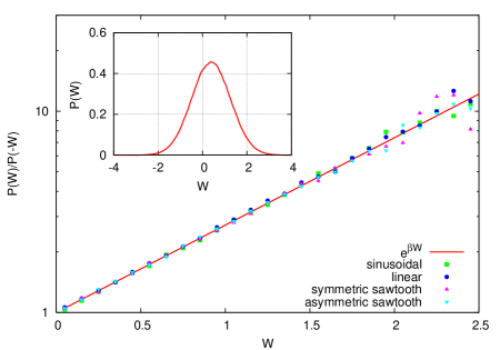
Figure 1: (Color online) The inset shows the work probability distribution $P(W)$ for a harmonic oscillator under a driving force $f(t)=sin(\pi t/\tau)$ and a bath with exponentially correlated noise. Simulation details are given in Sec. IV. The distribution is a Gaussian with a positive mean, but with significant amplitudes for negative $W$. Work probability distributions for other driving forces are qualitatively similar, as is $P(W_{diss})$. The main figure shows a log-lin plot of $P(W)/P(-W)$ versus $W$. The different points are for a variety of driving forces and their excellent agreement with the exponential confirms the validity of the TFT.

IV Anharmonic Oscillators

For anharmonic oscillators, finding simple expressions for $P(W)$ and $P(W_{J})$ is, in general, not possible; $W$ and $W_{J}$ are not linear combinations of the Gaussian stochastic quantities, therefore their distributions are not Gaussian. In this section, we numerically measure the work distribution functions for oscillators with the potential of Eq.(7) when $k_{3},k_{4}\geq 0$.

Random uncorrelated Gaussian numbers are commonly numerically generated and used in standard integration algorithms for Langevin equations of motion. An efficient Verlet-like integrator for second order white noise Langevin equations is given in Ref. verlet . We modify this algorithm in order to simulate Langevin systems with exponentially correlated noise. The damping kernel has the form

$$\gamma(t)=e^{-\Gamma|t|}.$$ (31)

Exponentially correlated noise can be effectively introduced by using white noise in the equation of motion for an auxiliary variable $z$, in addition to the position $x$ and velocity $v$. The coupled differential equations are

$$dx/dt = v,$$

$$dv/dt = -dV(x)/dx+f(t)+z,$$

$$dz/dt = -\Gamma z-v+\zeta.$$ (32)

$\zeta$ represents Gaussian white noise which is easily generated numerically,

$$<\zeta(t)>=0,\qquad<\zeta(t)\zeta(t^{\prime})>=2T\delta(t-t^{\prime}).$$ (33)

It can be shown that the equations of motion Eqs.(32) are equivalent to Eq.(5) with exponentially correlated noise Eq.(31). In all simulations, $T=\Gamma=\omega_{o}^{2}=1$, though we have verified that our results are qualitatively the same with different temperatures and damping constants. We use a step size $h$ with $h=0.01$ in all simulations shown. We have checked that our results do not change with smaller step sizes.

Work distributions are approximated by histograms of $O(10^{6})$ measurements of the work done ($W$ and $W_{J}$) over a time $\tau$. Between each measurement, we allow the oscillator to equilibrate by integrating Eqs.(32) for $O(10^{5})$ steps with $f(t)=0$. No differences in the distributions are seen for different histogram bin sizes and longer equilibration times.

We use a sawtooth driving force of the form,

$$f(t) = t/t_{o},\qquad 0\leq t\leq t_{o}$$ (34)

$$= (-t+\tau)/(\tau-t_{o}),\qquad t_{o}<t\leq\tau.$$

Under this driving force, the equilibrium configurations at $t=0$ and $t=\tau$ are identical, i.e. $\Delta F=0$ and $W=W_{J}$. In the $\tau\rightarrow 0$ limit, the work distribution is trivially peaked at $W=0$ because there is no time for work to be done. $P(W)$ is similarly peaked at zero in the $\tau\rightarrow\infty$ limit because the system is driven adiabatically from an equilibrium state back to the same equilibrium state. Our numerical simulations are in accord with these physical limits. The figures show simulation results with $\tau=10$, which is intermediate between these two limits. (No qualitative differences in terms of the JE, TFT, and CT exist with different $\tau$.) Lastly, $f(0)=0$, which is a necessary condition for the validity of the TFT for the harmonic oscillator detailed in the last section and Figure 1.

By changing $t_{o}$, we can alter the symmetry of $f(t)$; the force is symmetric in time only when $t_{o}=0.5\tau$. We implement this symmetric driving and two asymmetric sawtooth forces with $t_{o}=0.25\tau,0.75\tau$ in our simulations. As mentioned in the introduction, there is a subtle difference in the TFT and the CT with the latter using a time-reversed process in the denominator of the ratio of probabilities. For the symmetric sawtooth force, forward and reverse driving must be equivalent and no differences exist between the TFT and the CT. Our asymmetric sawtooth forces are complementary in that the time-reverse driving of one force is equivalent to the time-forward driving of the other. In other words, in terms of this sawtooth force, the TFT is

$$\frac{P_{t_{o}}(+W)}{P_{t_{o}}(-W)}=e^{+\beta W},$$ (35)

whereas the CT is

$$\frac{P_{t_{o}}(+W)}{P_{\tau-t_{o}}(-W)}=e^{+\beta W}.$$ (36)

($P_{s}(W)$ is the work distribution corresponding to a saw-tooth potential with a break at time $t=s$.)

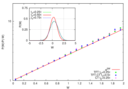
Figure 2: (Color online) The inset shows the work probability distributions for oscillators with quartic anharmonicities under sawtooth driving with $t_{o}/\tau=0.25,0.5,$ and $0.75$. These distributions have positive means, but also substantial weight on the negative region of $W$. $P_{0.25\tau}(W)=P_{0.75\tau}(W)$, indicating that the asymmetry in the driving force does not alter the work distribution functions, thus the ratios in the definition of the TFT and the CT, Eq.(35) and Eq.(36), must also be equal. The main figure confirms this equality and shows that the TFT and the CT are valid for the quartic oscillator.

We first simulate an anharmonic spring with a unit quartic anharmonicity (i.e. $k_{3}=0,k_{4}=1$). Figure 2 displays the results of these simulations. Aside from not being Gaussian, the probability distributions have similar properties as the work distribution of the harmonic oscillator: the means are all positive and there is a very substantial probability of measuring negative work. Furthermore, the two complementary asymmetric driving forces give the same work probability functions. From Eq.(35) and Eq.(36), it is clear that, in this case, the TFT and the CT are equivalent. The main plot in Fig. 2 displays this equality as well as the validity of the theorems.

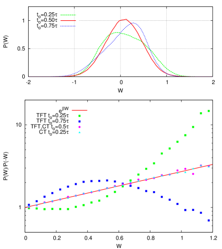
Figure 3: (Color online) The top panel shows the work probability distributions for particles in an asymmetric potential under sawtooth driving with $t_{o}/\tau=0.25,0.5,$ and $0.75$. Due to the lack of symmetry in the potential, $P_{0.25\tau}(W)\neq P_{0.75\tau}(W)$. The bottom panel shows the ratios from Eq.(35) and Eq.(36) versus $W$ on a log-lin plot. The data sets that agree with the exponential indicate that the CT is valid even for asymmetric potentials. The other sets indicate that the TFT fails for these potentials under general driving forces.

When a cubic nonlinearity is included ($k_{3}=k_{4}=1$), the even symmetry of the potential is broken. Figure 3 displays results for these non-symmetric oscillators. The top plot is analogous to the inset of Fig. 2 and shows the probability distributions for the three different sawtooth driving forces. From this figure, it is clear that all three distributions are different and the ratio in the TFT Eq.(35) is not equivalent to the ratio in the CT Eq.(36).

The difference between the TFT and the CT is clearly shown by the bottom panel of Fig. 3. In fact, the CT is valid under all sawtooth driving forces, whereas the TFT is only valid in the symmetric driving force. For oscillator potentials that are not symmetric in $x$, i.e. $V(x)\neq V(-x)$, and the driving force is asymmetric in time about $\tau/2$, the TFT dramatically fails.

For our example the validity of the JE follows from the CT. Independently, we have also measured the average exponential of the work and find $<e^{-\beta W}>=1$ within $\sim 4$ decimal places for both symmetric and asymmetric oscillators. Because $\Delta F=0$, this indicates the Jarzynski equality Eq.(2) is most likely valid for a large class of oscillator potentials, even with exponentially correlated noise.

When a sinusoidal force of the form $f(t)=sin(n\pi t/\tau)$, where $n$ is an odd integer, is used, the simulation results are qualitatively the same as with the symmetric sawtooth force. Obviously, this is because the period of the sinusoidal force gives a symmetric (about $\tau/2$) driving process. We also simulate linear driving which takes the system to a different equilibrium configuration in the adiabatic limit. Though $\Delta F\neq 0$ with linear driving, we find that the JE and the CT are still valid, but the TFT fails. This last result is not surprising because the linear driving force has many qualitative similarities with asymmetric sawtooth driving forces.

The above results are unchanged when colored noise is replaced by white noise. The white noise results are to be expected due to the numerous analytical derivations of these nonequilibrium theorems jarzynski ; crooks ; ND ; markov1 ; markov2 ; markov3 for Markovian baths. Our simulation results shown in this section indicate that the CT and the JE are also valid for non-Markovian baths.

V Summary

We have derived non-equilibrium work fluctuation theorems for the classical harmonic oscillator connected to a generalized Langevin bath by studying the work distribution functions of the real mechanical work and the Jarzynski generalized work. Both $W$ and $W_{J}$ are Gaussian variables. We derive the TFT for the real work and the JE by using exact relations between $<W>$ and $\sigma^{2}$ and $<W_{J}>$ and $\sigma_{J}^{2}$. To our knowledge, these are the first rigorous derivations of the nonequilbrium work fluctuation theorems for a system described by an arbitrary damping kernel of the generalized Langevin equation.

We also numerically measure the work distribution functions for anharmonic oscillators in Langevin baths with exponentially correlated noise. Our numerical simulations indicate that the JE extends to particles in a variety of oscillator potentials and driving forces. They also show that the symmetries of the potential and the driving force account for differences between the TFT and the CT. Crooks’ theorem is valid for all potentials and driving forces simulated, whereas the TFT is not valid when the oscillator potential is not even in $x$ and the driving force is not symmetric in $t$ (about $\tau/2$). The strong agreement between our simulation results and the nonequilibrium theorems (CT and JE) provides motivation for a derivation of the theorems for anharmonic oscillators in non-Markovian baths.

These results are important due to the existence of noise correlations in any real heat bath. This has obvious consequences for experimental tests of the Jarzynski equality and the fluctuation theorems. Experimentally, the JE is a powerful tool to measure equilibrium free energy differences due to the fact that any real driving is done irreversibly. Interesting and open questions still exist on the ramifications of the nonequilibrium fluctuation theorems and the second law “violating” events for molecular engines and microscopic thermodynamics.

References

- (1) C. Bustamante, J. Liphardt and F. Ritort, Physics Today 43 (July 2005).
- (2) D.J. Evans, E.G.D. Cohen, and G.P. Moriss, Phys. Rev. Lett. 71, 2401 (1993); D.J. Evans and D.J. Searles, Phys. Rev. E 50, 1645 (1994).
- (3) G. Gallavotti and E. G. D. Cohen, Phys. Rev. Lett. 74, 2694 (1995).
- (4) C. Jarzynski, Phys. Rev. Lett. 78, 2690 (1997); C. Jarzynski, J. Stat. Mech: Theor. Exp. P09005 (2004).
- (5) C. Jarzynski, Phys. Rev. E 56, 5018 (1997);
- (6) G.E. Crooks, Phys. Rev. E 60, 2721 (1999).
- (7) O. Narayan and A. Dhar, J. Phys. A 37, 63 (2004).
- (8) J. Kurchan, J. Phys. A 31, 3719 (1998).
- (9) J.L. Lebowitz and H. Spohn, J. Stat. Phys. 95, 333 (1999).
- (10) C. Maes, J. Stat. Phys. 95, 367 (1999).
- (11) G.M. Wang, E.M. Sevick, E. Mittag, D.J. Searles, D.J. Evans, Phys. Rev. Lett. 89, 050601 (2002). G.M. Wang, J.C. Reid, D.M. Carberry, D.R.M. Williams, E.M. Sevick, D.J. Evans, Phys. Rev E 71, 046142 (2005). K. Feitosa and N. Menon, Phys. Rev. Lett. 92, 164301 (2004). N. Garnier and S. Ciliberto, Phys. Rev. E. 71, 060101(R) (2005).
- (12) J. Liphardt, S. Dumont, S. Smith, I. Tinoco, and C. Bustamante, Science 296, 1832 (2002).
- (13) F. Douarche, S. Joubaud, N.B. Garnier, A. Petrosyan, S. Ciliberto Phys. Rev. Lett. 97, 140603 (2006).
- (14) A. Dhar, Phys. Rev. E 71, 036126 (2005).
- (15) R. Zwanzig Nonequilibrium Statistical Mechanics (Oxford University Press, 2001).
- (16) P. Hanggi, Lect. Notes Phys. 484, 15 (1997). U. Weiss, Quantum Dissipative Systems (Second Edition, World Scientific, 1999).
- (17) H. Mori, Prog. Theor. Phys. 33, 423 (1965). R. Kubo, Rep. Prog. Theor. Phys. 29, 255 (1966).
- (18) M.P. Allen and D.L. Tildesley, Computer Simulation of Liquids (Clarendon Press Oxford, 1987).