Finite-size scaling of the $d=5$ Ising model embedded in the cylindrical geometry: An influence of the hyperscaling violation

Abstract

Finite-size scaling (FSS) of the five-dimensional ($d=5$) Ising model is investigated numerically. Because of the hyperscaling violation in $d>4$, FSS of the $d=5$ Ising model no longer obeys the conventional scaling relation. Rather, it is expected that the FSS behavior depends on the geometry of the embedding space (boundary condition). In this paper, we consider the cylindrical geometry, and explore its influence on the correlation length $\xi=L^{\Omega}f(\epsilon L^{y^{*}_{t}},HL^{y^{*}_{h}})$ with system size $L$, reduced temperature $\epsilon$, and magnetic field $H$; the indices, $y^{*}_{t,h}$, and $\Omega$, characterize FSS. For that purpose, we employed the transfer-matrix method with Novotny’s technique, which enables us to treat an arbitrary (integral) number of spins $N=8,10,\dots,28$; note that conventionally, $N$ is restricted in $N(=L^{d-1})=16,81,256,\dots$. As a result, we estimate the scaling indices as $\Omega=1.40(15)$, $y^{*}_{t}=2.8(2)$, and $y^{*}_{h}=4.3(1)$. Additionally, under postulating $\Omega=4/3$, we arrive at $y^{*}_{t}=2.67(10)$ and $y^{*}_{h}=4.0(2)$. These indices differ from the naively expected ones, $\Omega=1$, $y^{*}_{t}=2$ and $y^{*}_{h}=3$. Rather, our data support the generic formulas, $\Omega=(d-1)/3$, $y^{*}_{t}=2(d-1)/3$, and $y^{*}_{h}=d-1$, advocated for the cylindrical geometry in $d\geq 4$.

I Introduction

The criticality of the Ising model above the upper critical dimension ($d>4$) belongs to the mean-field universality class. However, the finite-size effect, namely, the finite-size-scaling behavior, is not quite universal because of the violation of the hyperscaling in $d>4$. (From a renormalization-group viewpoint, this peculiarity is attributed to the presence of “dangerous irrelevant variable” Vladimir83 ; Privman83 ; Privman84 .) Actually, it is expected that the embedding geometry of the system (boundary condition) would affect the finite-size-scaling behavior for $d>4$ Brezin82 ; Brezin85 ; Privman90 ; Binder85 ; Binder85b ; Parisi96 ; Lai90 ; Kenna91 .

Recently, Jones and Young performed an extensive Monte Carlo simulation for the $d=5$ Ising model embedded in the (periodic) hypercubic geometry Jones05 . They calculated the correlation length $\xi$ with Kim’s technique Kim93 . (Because the calculation of $\xi$ requires a computational effort, Binder’s cumulant ratio rather than $\xi$ has been studied extensively so far Binder85 ; Binder85b ; Parisi96 .) They found that the correlation length $\xi$ obeys the scaling relation,

$$\xi=L^{\Omega}f(\epsilon L^{y^{*}_{t}}),$$ (1)

with the linear dimension $L$ and the reduced temperature $\epsilon$. They found that the scaling indices are in good agreement with the theoretical prediction Brezin82 ; Brezin85 ; Privman90 ,

$$\Omega=5/4\ and\ y^{*}_{t}=5/2.$$ (2)

Notably enough, their indices exclude the naively expected values, $\Omega=1$ and $y^{*}_{t}=2$. That is, the correlation length $\xi\sim L^{\Omega}$ exceeds the system size $L$ at the critical point $\epsilon=0$ as $L\to\infty$. (In other words, the spin-wave excitation costs very little energy for large $L$.) Such a peculiarity should be attributed to the violation of the conventional scaling relation (hyperscaling) in $d>4$. It would be intriguing that the above formula is cast into the expression Binder85 ,

$$\xi=lf(\epsilon l^{2}),$$ (3)

with the replacements $l=L^{\Omega}$ and $y^{*}_{t}=2\Omega$. The expression is now reminiscent of the conventional scaling relation expected for the mean-field universality class. Namely, the violation of hyperscaling is reconciled (absorbed) by the replacements, and the scaling indices, $\Omega$ and $y^{*}_{t}$, characterize the anomaly quantitatively. So far, numerous considerations have been made Binder85 ; Binder85b ; Parisi96 ; Jones05 for the hypercubic geometry, where the Monte Carlo method works very efficiently.

In this paper, we investigate the $d=5$ Ising model embedded in the cylindrical geometry; namely, we consider a system with infinite system size along a particular direction. Clearly, the transfer-matrix method well suits exploiting such a geometry. However, practically, the transfer-matrix method does not apply very well in large dimensions $d\geq 3$ because of its severe limitation as to the available system sizes.

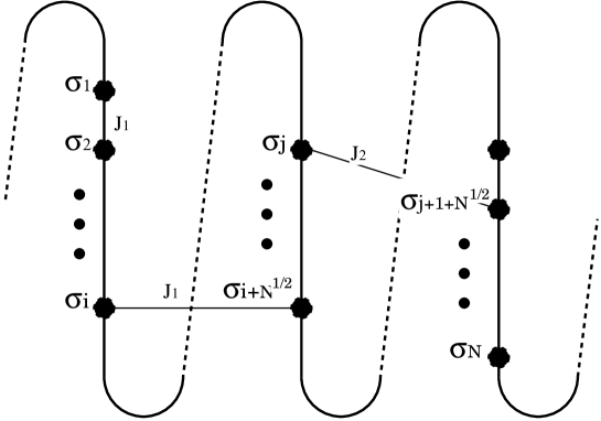
Figure 1: Construction of the spin cluster for the quantum transverse-field Ising model, Eq. (5). For simplicity, we consider the case of $d=2$. As indicated above, the spins constitute a $d=1$-dimensional alignment $\{\sigma_{i}\}$ ($i=1,2,\dots,N$), and the dimensionality is lifted to $d=2$ by introducing the bridges (long-range interactions) over the $N^{1/2}$th and $1+N^{1/2}$th neighbor pairs; these interactions correspond to the nearest-neighbor and the next-nearest-neighbor interactions, respectively, with respect to the $d=2$ cluster. In the case of $d=4$, we consider the $N^{1/4}$th, $N^{1/2}$th and $N^{3/4}$th neighbor interactions; see Eq. (8) for detail. This idea, namely, Novotny’s method, was first developed for the classical Ising model Novotny90 . We apply this method to the quantum system.

In order to resolve this limitation, we implemented Novotny’s technique Novotny90 ; Novotny92 ; Novotny93 ; Novotny91 ; Nishiyama04 , which enables us to treat an arbitrary number of system sizes $N=8,10,\dots,28$; here, the system size $N$ denotes the number of constituent spins within a unit of the transfer matrix (Fig. 1). Note that conventionally, the system size is restricted in $N(=L^{d-1})=16,81,256,\dots$, which soon exceeds the limit of available computer resources. Such an arbitrariness allows us to treat a variety of system sizes, and manage systematic finite-size-scaling analysis. Actually, with the scaling analysis, we obtained the indices $\Omega=1.40(15)$, $y^{*}_{t}=2.8(2)$, and $y^{*}_{h}=4.3(1)$. Moreover, postulating $\Omega=4/3$, we obtained $y^{*}_{t}=2.67(10)$ and $y^{*}_{h}=4.0(2)$. (Here, the exponent $y^{*}_{h}$ denotes the scaling dimension of the magnetic field. Our scaling relation, Eq. (13), incorporates the magnetic field $H$ and the corresponding scaling index $y^{*}_{h}$.) Obviously, our results exclude the naively expected ones, $\Omega=1$, $y^{*}_{t}=2$, and $y^{*}_{h}=3$. Rather, our data seem to support the generic formulas Brezin82 ; Brezin85 ; Privman90 ,

$$\Omega=\frac{d-1}{3},\ y^{*}_{t}=2\frac{d-1}{3},\ and\ y^{*}_{h}=d-1,$$ (4)

advocated for the cylindrical geometry in $d\geq 4$. Actually, our data deviate from the above mentioned values for the hypercubic geometry, Eq. (2), indicating that the embedding geometry is indeed influential upon the finite-size scaling.

In fairness, its has to be mentioned that Novotny obtained $\Omega+y^{*}_{t}\approx d-1$ Novotny90 ; Novotny91 . He postulated $\Omega=(d-1)/3$ in order to fix the location of the critical point. In this paper, we do not rely on any propositions, and estimate the indices independently. For that purpose, we calculated the cumulant ratio to get information on the critical point. Moreover, we treated the system sizes up to $N=28$, which is substantially larger than that of Ref. Novotny91 , $N\leq 13$. Here, we made use of an equivalence between the $d=5$ Ising model and the quantum $d=4$ Ising model; the latter is computationally less demanding. We also eliminated insystematic finite-size corrections by tuning extended coupling constants; see our Hamiltonian (5). In this respect, the motivation of the present research is well directed to methodology.

The rest of this paper is organized as follows. In Sec. II, we explain our simulation scheme in detail. In Sec. III, we manage the finite-size-scaling analyses of the simulation data. In the last section, we present the summary and discussions.

II Numerical method

In this section, we explain the numerical method. First, we argue the reduction of the $d=5$ Ising model to the $d=4$ quantum transverse-field Ising model. The reduced (quantum mechanical) model is much easier to treat numerically. Second, we explicate Novotny’s transfer-matrix method. We place an emphasis how we extended his formalism to adopt the quantum-mechanical interaction.

II.1 Reduction of the classical $d=5$ Ising model to the $d=4$ quantum counterpart

The $d$-dimensional Ising model reduces to the $(d-1)$-dimensional transverse-field Ising model; in general, the $d$-dimensional classical system has its $(d-1)$-dimensional quantum counterpart Suzuki76 . Such a reduction is based on the observation that the transfer-matrix direction and the (quantum) imaginary-time evolution have a close relationship. Actually, the quantum Hamiltonian is an infinitesimal generator of the transfer matrix. Because the quantum Hamiltonian contains few non-zero elements, its diagonalization requires reduced computational effort. The significant point is that the universality class (criticality) is maintained through the mapping.

To be specific, we consider the following $d=4$ transverse-field Ising model with the extended interactions. The Hamiltonian is given by,

$${\cal H}=-J_{1}\sum_{\langle ij\rangle}\sigma^{z}_{i}\sigma^{z}_{j}-J_{2}\sum_{\langle\langle ij\rangle\rangle}\sigma^{z}_{i}\sigma^{z}_{j}-J_{3}\sum_{[ij]}\sigma^{z}_{i}\sigma^{z}_{j}-J_{4}\sum_{[[ij]]}\sigma^{z}_{i}\sigma^{z}_{j}-\Gamma\sum_{i}\sigma^{x}_{i}-H\sum_{i}\sigma^{z}_{i}.$$ (5)

Here, the operators $\{\sigma^{\alpha}_{i}\}$ denote the Pauli matrices placed at the $d=4$ hypercubic lattice points $i$. The parameters $\Gamma$ and $H$ stand for the transverse and longitudinal magnetic fields, respectively. The summations, $\sum_{\langle ij\rangle}$, $\sum_{\langle\langle ij\rangle\rangle}$, $\sum_{[ij]}$, and $\sum_{[[ij]]}$, run over all possible nearest-neighbor pairs, the next-nearest-neighbor (plaquette diagonal) pairs, the third-neighbor pairs, and the fourth-neighbor pairs, respectively. The parameters $\{J_{i}\}$ ($i=1,2,3,4$) are the corresponding coupling constants. Hereafter, we regard $J_{1}$ as a unit of energy ($J_{1}=1$), and tune the remaining coupling constants $J_{2,3,4}$ so as to eliminate the insystematic finite-size errors; see Sec. III.

We simulate the above $d=4$ quantum Ising model with the numerical diagonalization method. The diagonalization of such a high-dimensional system requires huge computer-memory space. In fact, the number of spins constituting the $d=4$ cluster increases very rapidly as $N=16,81,256,\dots$, overwhelming the available computer resources. In the next section, we resolve this difficulty through resorting to Novotny’s transfer-matrix formalism.

II.2 Constructions of the Hamiltonian matrix elements

In this section, we present an explicit representation for the Hamiltonian (5). We make use of Novotny’s method Novotny90 , which enables us to treat an arbitrary number of spins constituting a unit of the transfer matrix. Novotny formulated the idea for the classical Ising model. In this paper, we show that his idea is applicable to the quantum Ising model, Eq. (5), as well.

Before we commence a detailed discussion, we explain the basic idea of Novotny’s method. In Fig. 1, we presented a schematic drawing of a unit of the transfer matrix for the Ising model in $d=3$ (rather than $d=5$ for the sake of simplicity). Because the cross-section of the $d=3$-dimensional bar is $d=2$-dimensional, the transfer-matrix unit should have a $d=2$-dimensional structure. However, in Fig. 1, the spins $\{\sigma_{i}\}$ ($\sigma_{i}=\pm 1$, $i=1,2,\dots,N$) constitute a $d=1$-dimensional (zig-zag) structure. This feature is essential for us to construct the transfer-matrix unit with an arbitrary (integral) number of spins. The dimensionality is lifted to $d=2$ effectively by the long-range interactions over the $\sqrt{N}$th-neighbor pairs; owing to the long-range interaction, the $N$ spins constitute a $\sqrt{N}\times\sqrt{N}$ rectangular network. (The significant point is that the number $\sqrt{N}$ is not necessarily an integral nor rational number.) Similarly, the bridge over $(\sqrt{N}\pm 1)$th neighbor pairs introduces the next-nearest-neighbor (plaquette diagonal) couping with respect to the $\sqrt{N}\times\sqrt{N}$ network.

We apply this idea to the case of the $d=4$ quantum system. To begin with, we set up the Hilbert-space bases $\{|\sigma_{1},\sigma_{2},\dots,\sigma_{N}\rangle\}$ ($\sigma_{i}=\pm 1$) for the quantum spins $\{\sigma^{\alpha}_{i}\}$ ($i=1,2,\dots,N$). These bases diagonalize the operator $\sigma^{z}_{j}$; namely,

$$\sigma^{z}_{j}|\{\sigma_{i}\}\rangle=\sigma_{j}|\{\sigma_{i}\}\rangle,$$ (6)

holds.

We consider the one- and two-body interactions separately. Namely, we decompose the Hamiltonian (5) into two sectors,

$${\cal H}={\cal H}^{(2)}(\{J_{i}\})+{\cal H}^{(1)}(\Gamma,H).$$ (7)

The component ${\cal H}^{(2)}$ originates from the spin-spin interaction, which depends on the exchange couplings $\{J_{i}\}$. On the other hand, the contribution ${\cal H}^{(1)}$ comes from the single-spin terms, depending on the magnetic fields, $\Gamma$ and $H$.

First, we consider ${\cal H}^{(2)}$. This component concerns the mutual connectivity among the $N$ spins, and we apply Novotny’s idea to represent the matrix elements. We propose the following expression,

$${\cal H}^{(2)} = \frac{J_{1}}{2}\sum_{\tilde{\alpha}=\pm\alpha,\alpha\in A}H(\tilde{\alpha})+\frac{J_{2}}{2}\sum_{\alpha,\beta\in A}\sum_{\tilde{\alpha}=\pm\alpha}\sum_{\tilde{\beta}=\pm\beta}H(\tilde{\alpha}+\tilde{\beta})$$ (8)

$$+\frac{J_{3}}{2}\sum_{\alpha,\beta,\gamma\in A}\sum_{\tilde{\alpha}=\pm\alpha}\sum_{\tilde{\beta}=\pm\beta}\sum_{\tilde{\gamma}=\pm\gamma}H(\tilde{\alpha}+\tilde{\beta}+\tilde{\gamma})$$

$$+\frac{J_{4}}{2}\sum_{\tilde{\alpha}=\pm 1}\sum_{\tilde{\beta}=\pm N^{1/4}}\sum_{\tilde{\gamma}=\pm N^{1/2}}\sum_{\tilde{\delta}=\pm N^{3/4}}H(\tilde{\alpha}+\tilde{\beta}+\tilde{\gamma}+\tilde{\delta}).$$

Here, the set $A$ consists of the elements, $A=\{1,N^{1/4},N^{1/2},N^{3/4}\}$. The component $H(v)$ denotes the $v$th-neighbor interaction for the $N$-spin alignment,

$$H_{\{\sigma_{i}\},\{\tau_{i}\}}(v)=\langle\{\sigma_{i}\}|H(v)|\{\tau_{i}\}\rangle=\langle\{\sigma_{i}\}|TP^{v}|\{\tau_{i}\}\rangle,$$ (9)

with the exchange-interaction matrix,

$$\langle\{\sigma_{i}\}|T|\{\tau_{i}\}\rangle=-\sum_{k=1}^{N}\sigma_{k}\tau_{k},$$ (10)

and the translational operator $P$ satisfying,

$$P|\{\sigma_{i}\}\rangle=|\{\sigma_{i+1}\}\rangle,$$ (11)

under the periodic boundary condition. The insertion of $P^{v}$ beside the $T$ operation is a key element to introduce the coupling over the $v$th-neighbor pairs. The denominator $2$ in Eq. (8) compensates the duplicated sum.

Let us explain the meaning of the above formula, Eq. (8), more in detail. As shown in Fig. 1, in the case of $d=2$, we made bridges over $N^{1/2}$th-neighbor pairs to lift up the dimensionality to $d=2$ effectively. In the case of $d=4$, by analogy, we introduce the interaction distances such as $v=1,N^{1/4},N^{1/2}$ and $N^{3/4}$. The first term in Eq. (8) thus represents the nearest-neighbor interactions (with respect to the $d=4$-dimensional cluster). Similarly, the remaining terms introduce the long-range interactions. For example, the component $H(1+N^{1/4})$ introduces the next-nearest-neighbor (plaquette diagonal) interaction. We emphasize that the idea of Novotny is readily applicable to the quantum model. [In short, our (quantum mechanical) formulation is additive. On the contrary, Novotny’s original formulation is multiplicative, because his original formulation concerns the Boltzmann weight rather than the Hamiltonian itself.]

Lastly, we consider the one-body part ${\cal H}^{(1)}$. The matrix element is given by the formula,

$${\cal H}^{(1)}_{\{\sigma_{i}\},\{\tau_{i}\}}=\langle\{\sigma_{i}\}|{\cal H}^{(1)}|\{\tau_{i}\}\rangle.$$ (12)

The expression is quite standard, because the component ${\cal H}^{(1)}$ simply concerns the individual spins, and has nothing to do with the connectivity among them.

The above formulas complete our basis to simulate the quantum Hamiltonian (5) numerically. In the next section, we perform the numerical simulation for $N=8,10,\dots,28$.

III Numerical results

In Sec. II, we set up an explicit expression for the Hamiltonian (5); see Eqs. (8) and (12). In this section, we diagonalize the Hamiltonian for $N=8,10,\dots,28$ with the Lanczos algorithm. We calculated the first-excitation energy gap $\Delta E$ (rather than $\xi$). The scaling relation for $\Delta E$ is given by,

$$\Delta E=L^{-\Omega}g(\epsilon L^{y^{*}_{t}},HL^{y^{*}_{h}}),$$ (13)

because $\Delta E\sim 1/\xi$ holds. (As compared to Eq. (1), our scaling relation is extended to include the magnetic field $H$ as well as the corresponding scaling index $y^{*}_{h}$.) The reduced temperature $\epsilon$ is given by $\epsilon=\Gamma-\Gamma_{c}$ with the critical point $\Gamma_{c}$. Note that the linear dimension $L$ satisfies $L=N^{1/4}$, because the $N$ spins constitute the $d=4$-dimensional cluster.

We fix the interaction parameters to,

$$(J_{1},J_{2},J_{3},J_{4})=(1,0.15,0.05,0.05),$$ (14)

and scan the transverse magnetic field $\Gamma$. (We will also provide data for $(J_{1},J_{2},J_{3},J_{4})=(1,0,0,0)$ and $(1,0.1,0.1,0.05)$ as a reference.) The interaction parameters, Eq. (14), are optimal in the sense that the insystematic finite-size errors are suppressed satisfactorily.

III.1 Scaling behavior of Binder’s cumulant ratio and the transition point

Because the scaling relation, Eq. (13), contains a number of free parameters, it is ambiguous to determine these parameters simultaneously. Actually, in Ref. Novotny90 ; Novotny91 , the author fixed $\Omega=4/3$, to determine the index $y^{*}_{t}$.

In this paper, we estimate the scaling indices independently without resorting to any postulations. For that purpose, we calculated an additional quantity, namely, Binder’s cumulant ratio Binder81 ,

$$U=1-\frac{\langle M^{4}\rangle}{3\langle M^{2}\rangle^{2}},$$ (15)

to determine the location of $\Gamma_{c}$. Here, the brackets $\langle\dots\rangle$ denote the expectation value at the ground state. The magnetic moment $M$ is given by $M=\sum_{i=1}^{N}\sigma^{z}_{i}$. Because the cumulant ratio is dimensionless ($\Omega=0$), it obeys a simplified scaling relation;

$$U=\tilde{U}(\epsilon L^{y^{*}_{t}},HL^{y^{*}_{h}}).$$ (16)

Hence, the intersection point of the cumulant-ratio curves indicates a location of the critical point. The scaling relation for the cumulant ratio, Eq. (16), has been studied extensively for the $d=5$ hypercubic geometry with the Monte Carlo method Binder85 ; Binder85b ; Parisi96 ; Jones05 .

In Fig. 2, we plotted the cumulant ratio for various $\Gamma$ and $N=8,10,\dots,28$ with $H=0$ fixed; as mentioned above, we fixed the exchange-coupling constants $\{J_{i}\}$ to Eq. (14). From the scale-invariant (intersection) point of the curves in Fig. 2, we observe a clear indication of criticality at $\Gamma_{c}\approx 12.5$. In the subsequent analysis of Sec. III.2, we make use of this information to determine the scaling indices.

This is a good position to address why we fixed the exchange couplings to Eq. (14). As a comparison, we presented the cumulant ratio for various $\Gamma$ and $N=8,10,\dots,28$ in Fig. 3, where we tentatively turn off the extended couplings $J_{2,3,4}=0$. Clearly, the data are scattered as compared to those of Fig. 2. Such data scatter obscures the onset of the phase-transition point, and prohibits detailed data analysis of criticality. In order to improve the finite-size behavior, we surveyed the parameter space $\{J_{i}\}$, and found that the choice (14) is an optimal one. Such elimination of finite-size errors has been utilized successfully in recent numerical studies Blote96 ; Nishiyama06 .

III.2 Critical exponent $\Omega$

Provided by the information on $\Gamma_{c}$ (Fig. 2), we are able to determine the scaling indices from the scaling relation (13). In this section, we consider the index $\Omega$.

In Fig. 4, we plotted the approximate index,

$$\Omega(L_{1},L_{2})=-\frac{\left.\ln(\Delta E(N_{1})/\Delta E(N_{2}))\right|_{\Gamma=\Gamma_{c}(L_{1},L_{2})}}{\ln(L_{1}/L_{2})},$$ (17)

for $[2/(L_{1}+L_{2})]^{3}$ with $8\leq N_{1}<N_{2}\leq 28$; note that $L_{1,2}=N_{1,2}^{1/4}$ holds. The parameters are the same as those of Fig. 2. The approximate transition point $\Gamma_{c}(L_{1},L_{2})$ is given by the intersection point of the cumulant ratio for a pair of $(N_{1},N_{2})$; namely, it satisfies

$$U(N_{1},\Gamma_{c}(L_{1},L_{2}))=U(N_{2},\Gamma_{c}(L_{1},L_{2})).$$ (18)

The least-squares fit to these data yields $\Omega=1.403(46)$ in the thermodynamic limit. We carried out similar data analysis for $(J_{2},J_{3},J_{4})=(0.1,0.1,0.05)$, and obtained $\Omega=1.494(21)$. As an error indicator, we accept the difference between them. As a consequence we estimate the index as

$$\Omega=1.40(15).$$ (19)

Let us mention a number of remarks. First, our result excludes the naively expected one $\Omega=1$. Actually, the result $\Omega>1$ indicates that the correlation length $L^{\Omega}$ develops more rapidly than the system size $L$ enlarges. This feature may reflect the fact that the spin waves cost very little energy large $L$. Second, our result supports the generic formula $\Omega=4/3$, Eq. (4), advocated for the cylindrical geometry in $d\geq 4$ Brezin82 ; Brezin85 ; Privman90 . On the contrary, it deviates from that of the hypercubic geometry (2); we confirm this observation in the following sections. Lastly, the validity of the abscissa scale (extrapolation scheme), $1/L^{3}$, in Fig. 4 is not clear. In Sec III.4, we inquire into the validity of the extrapolation scheme.

III.3 Critical exponents $y^{*}_{t}$ and $y^{*}_{h}$

In Figs. 5 and 6, we plotted the approximate indices,

$$-\Omega(L_{1},L_{2})+y^{*}_{t}(L_{1},L_{2})=\frac{\left.\ln(\partial_{\Gamma}\Delta E(N_{1})/\partial_{\Gamma}\Delta E(N_{2}))\right|_{\Gamma=\Gamma_{c}(L_{1},L_{2})}}{\ln(L_{1}/L_{2})},$$ (20)

and,

$$-\Omega(L_{1},L_{2})+2y^{*}_{h}(L_{1},L_{2})=\frac{\left.\ln(\partial^{2}_{H}\Delta E(N_{1})/\partial^{2}_{H}\Delta E(N_{2}))\right|_{H=0,\Gamma=\Gamma_{c}(L_{1},L_{2})}}{\ln(L_{1}/L_{2})},$$ (21)

respectively, for $[2/(L_{1}+L_{2})]^{3}$ with $8\leq N_{1}<N_{2}\leq 28$; the parameters are the same as those of Fig. 2. The least-squares fit to these data yields the estimates, $-\Omega+y^{*}_{t}=1.396(21)$ and $-\Omega+2y^{*}_{h}=7.198(39)$, in the thermodynamic limit. Similarly for $(J_{2},J_{3},J_{4})=(0.1,0.1,0.05)$, we obtained $-\Omega+y^{*}_{t}=1.359(12)$ and $-\Omega+2y^{*}_{h}=7.211(24)$. Consequently, we estimate the scaling indices as $-\Omega+y^{*}_{t}=1.4(1)$ and $-\Omega+2y^{*}_{h}=7.2(1)$. Combining them with $\Omega=1.40(15)$, Eq. (19), we arrive at,

$$y^{*}_{t}=2.8(2),$$ (22)

and,

$$y^{*}_{h}=4.3(1).$$ (23)

Again, our data exclude the naively expected values, $y^{*}_{t}=2$ and $y^{*}_{h}=3$. Rather, our estimates are comparable with the generic formula, Eq. (4); actually, the estimate $y^{*}_{t}=2.8(2)$ is quite consistent with the prediction $y^{*}_{t}=8/3$, Eq. (4), whereas the result $y^{*}_{h}=4.3(1)$ and the formula $y^{*}_{h}=4$, Eq. (4), are rather out of the error margin. We attain more satisfactory agreement between the numerical result and the formula by the data analysis under the assumption $\Omega=4/3$ in the next section. On the contrary, our data conflict with the values, Eq. (2), anticipated for the hypercubic geometry. Hence, the data suggest that the embedding geometry is influential on the finite-size scaling above the upper critical dimension. We confirm this issue more in detail in the next section.

III.4 Scaling indices $y^{*}_{t}$ and $y^{*}_{h}$ under the assumption $\Omega=4/3$

In Sec. III.2, we obtained an estimate $\Omega=1.40(15)$ being in good agreement with the formula $\Omega=4/3$, Eq. (4). In this section, we assume $\Omega=4/3$ Brezin82 , and estimate the remaining indices $y^{*}_{t}$ and $y^{*}_{h}$ under this hypothesis.

In Fig. 7, we plotted the approximate index,

$$y^{*}_{t}(L_{1},L_{2})=\frac{\left.\ln(\partial_{\Gamma}U(N_{1})/\partial_{\Gamma}U(N_{2}))\right|_{\Gamma=\tilde{\Gamma}_{c}(L_{1},L_{2})}}{\ln(L_{1}/L_{2})},$$ (24)

for the abscissa scale $[2/(L_{1}+L_{2})]^{3}$ with $8\leq N_{1}<N_{2}\leq 28$; the parameters are the same as those of Figs. 4-6. Because we assumed $\Omega=4/3$ Brezin82 , we are able to determine the approximate critical point $\tilde{\Gamma}_{c}(L_{1},L_{2})$ from the fixed point of $L^{4/3}\Delta E(L)$; namely,

$$L_{1}^{4/3}\Delta E(N_{1},\tilde{\Gamma}_{c}(L_{1},L_{2}))=L_{2}^{4/3}\Delta E(N_{2},\tilde{\Gamma}_{c}(L_{1},L_{2})).$$ (25)

We notice that the data exhibit improved convergence to the thermodynamic limit. The least-squares fit to these data yields $y^{*}_{t}=2.671(49)$ in the thermodynamic limit. Similarly, we obtained $y^{*}_{t}=2.697(42)$ for $(J_{2},J_{3},J_{4})=(0.1,0.1,0.05)$. Consequently, we estimate,

$$y^{*}_{t}=2.67(10).$$ (26)

This result is consistent with the above estimate $y^{*}_{t}=2.8(2)$, Eq. (22), confirming the reliability of our analyses in Figs. 4-6. It is also in good agreement with the prediction $y^{*}_{t}=8/3$, Eq. (4). On the contrary, our estimate excludes the exponent $y^{*}_{t}=5/2$, Eq. (2), advocated for the hypercubic geometry.

Similarly, in Fig. 8, we plotted the approximate index,

$$y^{*}_{h}(L_{1},L_{2})=\frac{1}{2}\frac{\left.\ln(\partial_{H}^{2}U(N_{1})/\partial_{H}^{2}U(N_{2}))\right|_{H=0,\Gamma=\tilde{\Gamma}_{c}(L_{1},L_{2})}}{\ln(L_{1}/L_{2})},$$ (27)

for the abscissa scale $[2/(L_{1}+L_{2})]^{3}$ with $8\leq N_{1}<N_{2}\leq 28$; the parameters are the same as those of Figs. 4-6. The data exhibit an appreciable systematic finite-size deviation. The least-squares fit to these data yields $y^{*}_{h}=4.021(60)$. Similarly, we obtained $y^{*}_{h}=4.148(36)$ for $(J_{2},J_{3},J_{4})=(0.1,0.1,0.05)$. Consequently, we estimate,

$$y^{*}_{h}=4.0(2).$$ (28)

Again, the result is quite consistent with the prediction $y^{*}_{h}=4$, Eq. (4). In other worlds, this agreement indicates that the extrapolation scheme (abscissa scale) $1/L^{3}$ is sensible.

Let us mention a few remarks. First, the data in Figs. 7 and 8 exhibit suppressed finite-size corrections owing to the assumption $\Omega=4/3$. This feature was observed in Refs. Novotny90 ; Novotny91 , where the author estimated $y^{*}_{t}$ reliably under $\Omega=(d-1)/3$; see the Introduction. Our analysis shows that the assumption yields a reliable estimate for $y^{*}_{h}$ as well as $y^{*}_{t}$. Second, our data confirm the self-consistency of our analyses performed in Figs. 4-8. Particularly, the data justify the extrapolation scheme with the abscissa scale $1/L^{3}$. As a matter of fact, in Ref. Luijten96 , the authors observed notable finite-size corrections to the cumulant ratio $U$ obeying $L^{d-2y^{*}_{h}}$. In our case ($d=5$ cylindrical geometry), the power should read $d-2y_{h}^{*}=-3$. Hence, our numerical data support their claim. Lastly, as to the convergence of $U$ to the thermodynamic limit, there arose controversies Chen98 ; Chen98b ; Chen00 ; Luijten99 ; Binder00 ; Mon96 ; Luijten97 ; Mon97 ; Blote97 ; it has been reported that there appear unclarified finite-size corrections to $U$, which prohibit us to take reliable extrapolation to the thermodynamic limit. In this paper, we avoided the subtlety by eliminating finite-size errors with the (finitely-tuned) extended interactions; see Figs. 2 and 3. We consider that such a technique would be significant for the study of high-dimensional systems, where the available system size is restricted.

IV Summary and discussions

We studied the finite-size-scaling behavior of the $d=5$ Ising model embedded in the cylindrical geometry. Our aim is to see an influence of the embedding geometry (boundary condition) on the scaling relation, Eq. (13); the embedding geometry should alter the scaling indices $\Omega$ and $y^{*}_{t,h}$ above $d>4$ Brezin82 ; Brezin85 ; Privman90 . For that purpose, we employed the transfer-matrix method (Sec. II), and implemented Novotny’s technique Novotny90 to treat a variety of system sizes $N=8,10,\dots,28$. Moreover, we made use of an equivalence between the $d=5$ (classical) Ising model and its $d=4$ quantum counterpart; the latter version is computationally less demanding with the universality class retained.

We analyzed the simulation data with the finite-size scaling relation, Eq. (13), and obtained the scaling indices as $\Omega=1.40(15)$, $y^{*}_{t}=2.8(2)$, and $y^{*}_{h}=4.3(1)$. Additionally, under $\Omega=4/3$, we estimate $y^{*}_{t}=2.67(10)$ and $y^{*}_{h}=4.0(2)$. The indices exclude the naively expected ones, $\Omega=1$, $y^{*}_{t}=2$, and $y^{*}_{h}=3$, reflecting the violation of hyperscaling in large dimensions. Clearly, our data support the generic formulas, Eq. (4), advocated for the cylindrical geometry in $d\geq 4$ Brezin82 ; Brezin85 ; Privman90 . On the contrary, our data conflict with the values for the hypercubic geometry, Eq. (2). Our result demonstrates that the embedding geometry is indeed influential on the scaling indices.

Lastly, let us mention a few remarks. First, we stress that the violation of hyperscaling above the upper critical dimension $\tilde{d}$ is not necessarily an issue of pure academic interest. For example, a class of long-range interaction Luijten96 suppresses the upper critical dimension to an experimentally accessible regime $\tilde{d}<3$. Second, there arose controversies Chen98 ; Chen98b ; Chen00 ; Luijten99 ; Binder00 ; Mon96 ; Luijten97 ; Mon97 ; Blote97 concerning the subdominant finite-size effect (corrections to scaling) above $\tilde{d}$. More specifically, the Binder-cumulant data exhibit unexpectedly slow convergence to the thermodynamic limit. In this paper, we avoided this subtlety by extending (tuning) the exchange-coupling constants to Eq. (14), where we observed eliminated finite-size errors. Actually, from Figs. 2 and 3, we notice that the elimination was successful. Our data indicate that the (dominant) finite-size errors obey the power law $L^{-3}$ as claimed in Ref. Luijten96 . We consider that the elimination of finite-size errors is significant for the study of high-dimensional systems, where the available system size is restricted severely.

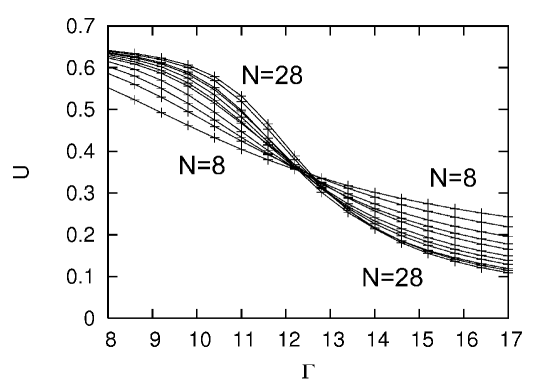
Figure 2: Binder’s cumulant ratio $U$ (15) is plotted for the transverse magnetic field $\Gamma$ and the system sizes $N=8,10,\dots,28$ with the fixed exchange couplings, Eq. (14). We observe a clear indication of criticality at $\Gamma_{c}\approx 12.5$. Apparently, the finite-size-scaling behavior is improved as compared to that of Fig. 3, where we turned off the extended interactions $J_{2,3,4}=0$.

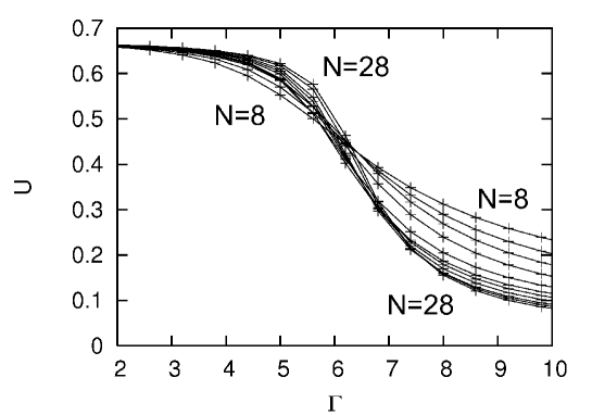
Figure 3: Tentatively, we turned off the extended interactions ($J_{2,3,4}=0$), and calculated the cumulant ratio $U$ (15) for various $\Gamma$ and $N=8,10,\dots,28$. We notice that the data are scattered as compared to those in Fig. 2.

Figure 4: The approximate critical index $\Omega(L_{1},L_{2})$ (17) is plotted for $[2/(L_{1}+L_{2})]^{3}$ with $8\leq N_{1}<N_{2}\leq 28$ ($L_{1,2}=N_{1,2}^{1/4}$); the parameters are the same as those of Fig. 2. The least-squares fit to these data yields $\Omega=1.403(46)$ in the thermodynamic limit $L\to\infty$.

Figure 5: The approximate critical index $-\Omega(L_{1},L_{2})+y^{*}_{t}(L_{1},L_{2})$ (20) is plotted for $[2/(L_{1}+L_{2})]^{3}$ with $8\leq N_{1}<N_{2}\leq 28$ ($L_{1,2}=N_{1,2}^{1/4}$); the parameters are the same as those of Fig. 2. The least-squares fit to these data yields $-\Omega+y^{*}_{t}=1.396(21)$ in the thermodynamic limit $L\to\infty$.

Figure 6: The approximate critical index $-\Omega(L_{1},L_{2})+2y^{*}_{h}(L_{1},L_{2})$ (21) is plotted for $[2/(L_{1}+L_{2})]^{3}$ with $8\leq N_{1}<N_{2}\leq 28$ ($L_{1,2}=N_{1,2}^{1/4}$); the parameters are the same as those of Fig. 2. The least-squares fit to these data yields $-\Omega+2y^{*}_{h}=7.198(39)$ in the thermodynamic limit $L\to\infty$.

Figure 7: The approximate critical index $y^{*}_{t}(L_{1},L_{2})$ (24) is plotted for $[2/(L_{1}+L_{2})]^{3}$ with $8\leq N_{1}<N_{2}\leq 28$ ($L_{1,2}=N_{1,2}^{1/4}$); the parameters are the same as those of Fig. 2. The least-squares fit to these data yields $y^{*}_{t}=2.671(49)$ in the thermodynamic limit $L\to\infty$. The result is consistent with Eq. (22), confirming the reliability of our analysis.

Figure 8: The approximate critical index $y^{*}_{h}(L_{1},L_{2})$ (27) is plotted for $[2/(L_{1}+L_{2})]^{3}$ with $8\leq N_{1}<N_{2}\leq 28$ ($L_{1,2}=N_{1,2}^{1/4}$); the parameters are the same as those of Fig. 2. The least-squares fit to these data yields $y^{*}_{h}=4.021(60)$ in the thermodynamic limit $L\to\infty$. The result is consistent with the prediction (4).

- (1) V. Vladimir and M. E. Fisher, J. Stat. Phys. 33, 385 (1983).
- (2) V. Privman and M. E. Fisher, J. Phys. A 16, l295 (1983).
- (3) V. Privman and M. E. Fisher, Phys. Rev. B 30, 322 (1984).
- (4) E. Brézin, J. Phys. (France) 43, 15 (1982).
- (5) E. Brézin and J. Zinn-Justin, Nucl. Phys. B 257, 867 (1985).
- (6) V. Privman, Finite Size Scaling and Numerical Simulation of Statistical Systems, Ed. V. Privman (World Scientific, Singapore, 1990).
- (7) K. Binder, Z. Phys. B 61, 13 (1985).
- (8) K. Binder, M. Nauenberg, V. Privman, and A. P. Young, Phys. Rev. B 31, 1498 (1985).
- (9) G. Parisi and J. J. Ruiz-Lorenzo, Phys. Rev. B 54, R3698 (1996).
- (10) P.-Y. Lai and K. K. Mon, Phys. Rev. B 41, 9257 (1990).
- (11) R. Kenna and C. B. Lang, Phys. Lett. B 264, 396 (1991).
- (12) J. L. Jones and A. P. Young, Phys. Rev. B 71, 174438 (2005).
- (13) J.-K. Kim, Phys. Rev. Lett. 70, 1735 (1993).
- (14) M.A. Novotny, J. Appl. Phys. 67, 5448 (1990).
- (15) M.A. Novotny, Phys. Rev. B 46, 2939 (1992).
- (16) M.A. Novotny, Phys. Rev. Lett. 70, 109 (1993).
- (17) M.A. Novotny, Computer Simulation Studies in Condensed Matter Physics III, edited by D.P. Landau, K.K. Mon, and H.-B. Schüttler (Springer-Verlag, Berlin, 1991).
- (18) Y. Nishiyama, Phys. Rev. E 70, 026120 (2004).
- (19) M. Suzuki, Prog. Theor. Phys. 56, 1454 (1976).
- (20) K. Binder, Phys. Rev. Lett. 47, 693 (1981).
- (21) H. W. J. Blöte, J. R. Heringa, A. Hoogland, E. W. Meyer, and T. S. Smit, Phys. Rev. Lett. 76, 2613 (1996).
- (22) Y. Nishiyama, Phys. Rev. E 74, 016120 (2006).
- (23) E. Luijten and H. W. J. Blöte, Phys. Rev. Lett. 76, 1557 (1996); ibid., 76, 3662 (1996) (E).
- (24) X. S. Chen and V. Dohm, Physica A 251, 439 (1998).
- (25) X. S. Chen and V. Dohm, Int. J. Mod. Phys. C 9, 1007 (1998).
- (26) X. S. Chen and V. Dohm, Phys. Rev. E 63, 016113 (2000).
- (27) E. Luijten, K. Binder, and H. W. J. Blöte, Eur. Phys. J. B 9, 289 (1999).
- (28) K. Binder, E. Luijten, M. Müller, N. B. Wilding, and H. W. J. Blöte, Physica A 281, 112 (2000).
- (29) K. K. Mon, Europhys. Lett. 34, 388 (1996).
- (30) E. Luijten, Europhys. Lett. 37, 489 (1997).
- (31) K. K. Mon, Europhys. Lett. 37, 493 (1997).
- (32) H. W. J. Blöte and E. Luijten, Europhys. Lett. 38, 565 (1997).