Higher angular momentum Kondo liquids

Abstract

Conventional heavy Fermi liquid phases of Kondo lattices involve the formation of a “Kondo singlet” between the local moments and the conduction electrons. This Kondo singlet is usually taken to be in an internal s-wave angular momentum state. Here we explore the possibility of phases where the Kondo singlet has internal angular momentum that is d-wave. Such states are readily accessed in a slave boson mean field formulation, and are energetically favorable when the Kondo interaction is between a local moment and an electron at a nearest neighbor site. The properties of the d-wave Kondo liquid are studied. Effective mass and quasiparticle residue show large angle dependence on the Fermi surface. Remarkably in certain cases, the quasiparticle residue goes to zero at isolated points (in two dimensions) on the Fermi surface. The excitations at these points then include a free fractionalized spinon. We also point out the possibility of quantum Hall phenomena in two dimensional Kondo insulators, if the Kondo singlet has complex internal angular momentum. We suggest that such d-wave Kondo pairing may provide a useful route to thinking about correlated Fermi liquids with strong anisotropy along the Fermi surface.

I Introduction

In many rare earth alloys, a periodic lattice of localized spin-$1/2$ magnetic moments is coupled through Kondo exchangeKondo (1966) to a separate band of conduction electronsDoniach (1977). An interesting low temperature metallic phase often develops at low temperature where the local moments are absorbed into the Fermi sea by a lattice analog of the Kondo effect. The resulting metallic phase is a Fermi liquid albeit with strongly renormalized parameters the most dramatic of which is a large quasiparticle mass enhancement (leading to the name ‘heavy fermi liquid’). Concomittantly the quasiparticle residue at the Fermi surface is very small (though non-zero). Perhaps most strikingly the Fermi surface is large in the sense that its volume satisfies Luttinger’s theoremLuttinger (1960) only if the local moments are included in the count of the electron density. This and other universal properties of this Fermi liquid are usefully understood in a strong Kondo coupling picture where each conduction electron is trapped into a spin singlet state with a local moment - see Ref. Nozieres, 1998.

The singlet ‘molecule’ formed out of the local moment and conduction electron is usually taken to be in an s-wave state with zero internal angular momentum. In this paper we explore metallic states where this singlet has non-zero internal angular momentum. We show that this results in Fermi liquid states that have many unusual and interesting properties. For instance such states naturally have large anisotropies in the effective mass, quasiparticle residue and other properties on moving around the Fermi surface. Under certain conditions it is even possible for the quasiparticle residue to vanish at isolated points of the Fermi surface. The excitations at such points do not have electron quantum numbers but can be understood as a neutral fermionic spin-$1/2$ ‘spinon’. Remarkably such a spinon excitation emerges without any associated gauge interaction (unlike the other many familiar examplesRead and Sachdev (1991); Wen (1991); Senthil and Fisher (2000)). In the special case where the conduction band is half-filled the usual s-wave Kondo singlet formation leads to an insulating state (dubbed the Kondo insulator). If the internal angular momentum is non-zero, interesting varieties of Kondo insulators become possible. For instance we show that in two dimensions with a $d_{x^{2}-y^{2}}+id_{xy}$ singlet, the Kondo insulator has a non-trivial quantized electrical Hall conductivity.

A partial motivation for studying such higher angular momentum singlet formation between local moments and conduction electrons comes from observations on cuprate high-$T_{c}$ materials. We should immediately emphasize though that the two band Kondo-lattice models are not directly expected to be an appropriate microscopic description of the cuprates. Nevertheless it seems worthwhile to point out some resemblances between the properties of the metallic states described in this paper and those seen in the cuprates. Extending the ideas of this paper to one-band models appropriate to the cuprates may be an interesting direction for future work. For some attempts along similar directions see Ref. Ribeiro and Wen, 2005. The optimally doped cuprates in the normal state are metallic and have a full Fermi surface satisfying the usual Luttinger theoremLee et al. (2006). Despite this however a true sharp electronic quasiparticle peak does not seem to exist. The electron spectrum - measured through photoemission experiments - shows significant anisotropy on moving around the Fermi surfaceZhou et al. (2004). In particular the energy distribution curve (EDC) is narrower along the nodal direction as compared to the antinodal direction. This kind of anisotropy in the EDC persists into the underdoped side when a pseudogap opens along the antinodal direction. It also persists into the superconducting state obtained by cooling. Collectively these phenomena have been dubbed the ‘nodal-antinodal dichotomy’: the nodal excitations are much more quasiparticle-like than the antinodal ones.

The general message from these results on the cuprates for the study of correlated metals is that correlation effects may not uniformly affect all parts of the Fermi surface in a metal. Some portions of the Fermi surface may be more susceptible to correlation effects than others. This will lead to strong correlation induced anisotropy in physical properties around the Fermi surface. Theoretically study of such effects is difficult because electron correlations are typically most easily handled in real space which does not readily distinguish between different parts of the Fermi surface. Interesting recent numerical calculationsCivelli et al. (2005) based on cluster extensions of dynamical mean field theory on single band Hubbard models in two dimensions have found such momentum space differentiation in the electronic properties. The ideas of the present paper may be seen as a step toward incorporating momentum space differentiation into simple analytic treatments of strong correlation problems. Anisotropic spectra at different regions of the Fermi surface occur naturally in the metallic states described in the two band Kondo lattice models studied in this paper.

Theoretically higher angular momentum Kondo liquids are conveniently accessed through the slave boson mean field theoryRead et al. (1984); Millis and Lee (1987) developed to describe the usual heavy fermi liquid state. In this theory the local moment $\vec{S}_{r}$ at site $r$ is represented in terms of neutral spin-$1/2$ fermions $f_{r\alpha}$ ($\alpha=\uparrow,\downarrow$)through

$$\vec{S}_{r}=\frac{1}{2}f^{\dagger}_{r}\vec{\sigma}f_{r}$$ (1)

The Kondo singlet formation is then signalled by the development of a non-zero expectation value of the singlet hybridization amplitude $\langle c^{\dagger}_{r}f_{r}\rangle$ between the $f$-fermions and conduction electrons $c_{r}$. This immediately suggests that Kondo singlets of higher angular momentum can be described by hybridization amplitudes between $f_{r}$ at site $r$ and $c_{r^{\prime}}$ at a different site $r^{\prime}$. Specifically

$$b_{rr^{\prime}}=\langle c^{\dagger}_{r}f_{r^{\prime}}\rangle$$ (2)

may be viewed as the wave function of the Kondo singlet. Thus by choosing the internal angular momentum associated with rotations of the relative coordinate $\vec{r}\ ^{\prime}-\vec{r}$ appropriately Kondo liquids with higher angular momentum may be constructed. In this paper we will exploit this strategy to construct mean field descriptions of various such Kondo liquid states. Within the mean field description, higher angular momentum Kondo liquids correspond to a particular form of momentum dependence of the Kondo hybridization amplitude. Momentum dependent hybridization amplitudes have been previously considered in Ref. Moreno and Coleman, 2000. Recent optical transport experiments on the 1-1-5 materials have also been interpreted in terms of momentum dependent hybridization amplitudesBurch et al. (a)Burch et al. (b).

We begin in Section II with a brief review of the usual slave boson mean field theory for a heavy fermi liquidColeman (2002). This mean field theory describes an on-site “s-wave” Kondo singlet. We then consider in Section III a Kondo lattice Hamiltonian where each local moment interacts through Kondo exchange with a conduction electron at a neighboring site. Within mean field theory this Hamiltonian is shown to stabilize a $d$-wave Kondo liquid. The properties of this state are then studied in Section IV. Next we modify the Kondo lattice model of Section III by introducing explicit Heisenberg exchange between nearest neighbor moments. A mean field treatment of this model (Section V) leads to a metallic state where the quasiparticle residue vanishes at isolated points of the Fermi surface. As mentioned above this remarkable state has spinon excitations at these isolated points without any associated gauge interactions. Next in Section VI we consider two dimensional Kondo insulators where the Kondo singlet has complex internal angular momentum of the form $d_{x^{2}-y^{2}}+id_{xy}$. We calculate the Hall conductivity and show that it has a non-trivial quantized value. Thus this provides an interesting example of a quantum Hall state in a Kondo lattice. Section VIII has some conclusions. various details are in the Appendices.

II Review of mean-field theory for Kondo liquid: s-Wave singlet

Consider the Kondo lattice model describing a lattice of spin-$1/2$ local moments $\vec{S}_{i}$ and conduction electrons $c_{i\alpha}$ $(\alpha=\uparrow,\downarrow)$ coupled through Kondo exchangeKondo (1966).

$$H=-\sum_{\langle ij\rangle}tc^{\dagger}_{i}c_{j}+\frac{J_{K}}{2}\sum_{i}\vec{S}_{i}.c^{\dagger}_{i}\vec{\sigma}c_{i}$$ (3)

The total number of conduction electrons per site is taken to be some fixed value $n_{c}$. We also specialize to two dimensional systems though extension to three dimension is straightforward. A useful mean field treatment is obtained using a fermionic representation of the local moment spin:

$$\vec{S}_{i}=f^{\dagger}_{i}\frac{\vec{\sigma}}{2}f_{i}$$ (4)

together with the constraint $f^{\dagger}_{i}f_{i}=1$ at each site. After some algebra the interaction term ($J_{K}$) reduces to:

$$\sum_{i}f_{i}^{\dagger}c_{i}c^{\dagger}_{i}f_{i}+constant$$

In the corresponding partition function, this takes the form

$$e^{\int d\tau\sum_{i}\bar{f}_{i}c_{i}\bar{c}_{i}f_{i}}$$ (5)

Using a Hubbard-Stratonovich transformation, this can be decoupled as

$$\int[DV]\ \exp\left(\sum_{i}\frac{|V(i,\tau)|^{2}}{4J_{k}}+(V(i,\tau)\bar{f}_{i}c_{i}+V^{*}(i,\tau)\bar{c}_{i}f_{i})\right)$$ (6)

Exact integration over $V(i,\tau)$ will produce the original interaction term. But in mean-field approximation, we do the integral using saddle-point method. In addition the constraint $f^{\dagger}_{i}f_{i}=1$ will be implemented on average. We will choose the mean-field solution with $V(i,\tau)=V$ which leads to the following mean-field Hamiltonian and self consistency equation for $V$:

$$H = -\sum_{\langle ij\rangle}tc^{\dagger}_{i}c_{j}+h.c$$ (7)

$$+\sum_{i}\mu_{f}f^{\dagger}_{i}f_{i}+V\sum_{i}(f^{\dagger}_{i}c_{i}+c^{\dagger}_{i}f_{i})$$

$$V = \frac{J_{k}}{2N}\sum_{i}\langle f^{\dagger}_{i}c_{i}+h.c.\rangle$$ (8)

$$\langle f^{\dagger}_{i}f_{i}\rangle = 1$$ (9)

We have introduced a chemical potential term for the $f$-fermions which serves to set their average number per site to be one. In addition the Fermi energy $E_{F}$ of the hybridized quasiparticle must be determined by requiring that there are a total of $1+n_{c}$ fermions per site. Only states with energy less than $E_{F}$ are filled in the ground state. This mean-field Hamiltonian is quadratic and can be diagonalized. To do so, first we write the Hamiltonian in the Fourier space:

$$H=\sum_{k}\epsilon_{\textbf{k}}c^{\dagger}_{\textbf{k}}c_{\textbf{k}}+\sum_{\textbf{k}}\mu_{f}f^{\dagger}_{\textbf{k}}f_{\textbf{k}}+V\sum_{\textbf{k}}(f^{\dagger}_{\textbf{k}}c_{\textbf{k}}+c^{\dagger}_{\textbf{k}}f_{\textbf{k}})$$ (10)

with $\epsilon_{\textbf{k}}=-2t\ (\cos(k_{x})+\cos(k_{y}))$. Now it is easy to derive quasi-particle dispersion relation for two bands:

$$E^{\pm}_{\textbf{k}}=\frac{\epsilon_{\textbf{k}}+\mu_{f}}{2}\pm\sqrt{(\frac{\epsilon_{\textbf{k}}-\mu_{f}}{2})^{2}+V^{2}}$$ (11)

With this in hand, we can solve the self consistency conditions and calculate physical properties. For instance the density of states at the Fermi energy is exponentially large in $1/J_{K}$ leading to the large mass enhancement at small $J_{K}$.

III d-wave Kondo liquid

In the last section we considered the case where the singlets between the local moments and conduction electrons are formed with zero internal angular momentum (i.e. $\langle f^{\dagger}_{i}c_{i}+h.c.\rangle$ is constant). When we assume that the singlet is formed between the local moments and conduction electron at the same site (i.e. singlet is local), the s-wave is the only possibility for internal state of the singlet. In this section we consider modifying the Kondo lattice Hamiltonian so that Kondo singlets with non-zero angular momentum are favored. To that end we consider a generalized Kondo Hamiltonian:

$$H=-\sum_{\langle ij\rangle}tc^{\dagger}_{i}c_{j}+\sum_{ij}J_{ij}\vec{S}_{i}.\vec{s}_{j}$$ (12)

where the Kondo exchange term is not limited to the local moments and conduction electrons at the same site. The simplest case is for $J_{ij}$ to be non-zero only when $i$ and $j$ denote the nearest neighbor sites:

$$J_{ij} = J_{K}~{}~{}~{}~{}(i,j)~{}\text{nearest neighbor}$$ (13)

$$J_{ij} = 0~{}~{}~{}~{}\text{otherwise}$$ (14)

With this choice and after some algebra, similar to what we did in the last section, the Hamiltonian reduces to the following form:

$$H=-\sum_{\langle ij\rangle}tc^{\dagger}_{i}c_{j}+\sum_{\langle ij\rangle}J_{ij}\ f^{\dagger}_{i}c_{j}c^{\dagger}_{j}f_{i}$$ (15)

Now proceed as before by decoupling the interacting part of the action using an auxiliary field, which this time lives on the bonds of the lattice, instead of the sites:

$$\begin{split}\int&[DV]\ \\ &e^{-\left(\int d\tau\sum_{\langle i,j\rangle}\frac{|V(i,j,\tau)|^{2}}{4J_{k}}+(V(i,j,\tau)\bar{f}_{i}c_{j}+V^{*}(i,j,\tau)\bar{c}_{j}f_{i})\right)}\end{split}$$ (16)

As before, to get the mean-field Hamiltonian, we’ll do the integration over $V$ using saddle point approximation (in addition to imposing $\langle f^{\dagger}_{i}f_{i}\rangle=1$ on average). There are different saddle point solutions (they are basically different local minima in functional space). We will consider two solutions named as s-wave and d-wave (the reason for choosing these names will become clear later). In s-wave solution we consider $V(i,j,\tau)=V$ on all bonds and in d-wave, we consider $V(i,j,\tau)=V$ on $x$ bonds and $V(i,j,\tau)=-V$ on $y$ bonds:

$$\begin{split}H_{\left(\begin{array}[]{ccc}s\\ d\end{array}\right)}=&\sum_{-\langle ij\rangle}tc^{\dagger}_{i}c_{j}+\sum_{i}\mu_{f}f^{\dagger}_{i}f_{i}+\\ &\sum_{i,x,y}V[(f_{i}^{\dagger}c_{i+x}+c^{\dagger}_{i+x}f_{i})\pm(f_{i}^{\dagger}c_{i+y}+c^{\dagger}_{i+y}f_{i})]\end{split}$$ (17)

It is obvious from this form that these correspond to s-wave and d-wave internal state for the singlet. In momentum space s-wave and d-wave Hamiltonian have the following forms:

$$\begin{split}H_{s}(\textbf{k})=\sum_{\textbf{k}}&\epsilon_{\textbf{k}}c^{\dagger}_{\textbf{k}}c_{\textbf{k}}+\sum_{\textbf{k}}\mu_{f}f^{\dagger}_{\textbf{k}}f_{\textbf{k}}\\ &+V\sum_{\textbf{k}}(\cos(k_{x})+\cos(k_{y}))(f^{\dagger}_{\textbf{k}}c_{\textbf{k}}+c^{\dagger}_{\textbf{k}}f_{\textbf{k}})\end{split}$$ (18)

$$\begin{split}H_{d}(k)=\sum_{k}&\epsilon_{\textbf{k}}c^{\dagger}_{\textbf{k}}c_{\textbf{k}}+\sum_{\textbf{k}}\mu_{f}f^{\dagger}_{\textbf{k}}f_{\textbf{k}}\\ &+V\sum_{\textbf{k}}(\cos(k_{x})-\cos(k_{y}))(f^{\dagger}_{\textbf{k}}c_{\textbf{k}}+c^{\dagger}_{\textbf{k}}f_{\textbf{k}})\end{split}$$ (19)

With this quadratic mean-field Hamiltonian, we can also derive the spectrum and the mean-field parameter $V$ self-consistently:

$$\begin{split}E^{s}_{\pm}({\textbf{k}})=&\frac{\epsilon_{\textbf{k}}+\mu_{f}}{2}\pm\\ &\sqrt{(\frac{\epsilon_{\textbf{k}}-\mu_{f}}{2})^{2}+V^{2}(\cos(k_{x})+\cos(k_{y}))^{2}}\end{split}$$ (20)

$$\begin{split}E^{d}_{\pm}({\textbf{k}})=&\frac{\epsilon_{\textbf{k}}+\mu_{f}}{2}\pm\\ &\sqrt{(\frac{\epsilon_{\textbf{k}}-\mu_{f}}{2})^{2}+V^{2}(\cos(k_{x})-\cos(k_{y}))^{2}}\end{split}$$ (21)

The ground state is obtained by filling all states upto the Fermi level. As before the Fermi energy is fixed by requiring that there are $1+n_{c}$ fermions in the ground state per site. Note that in both $s$ and $d$ wave cases the $+$ band lies entirely above the $-$ band (i.e $min(E_{+})\geq max(E_{-})$). Therefore in the ground state only the $E_{-}$ levels are occupied. The ground state energy is

$$E^{s,d}_{gd}=\sum_{k}\theta(E_{F}-E^{s,d}_{-}({\textbf{k}}))E^{s,d}_{-}({\textbf{k}})$$ (22)

The self-consistency equations that determine $V$ and $\mu_{f}$ are now readily obtained. For instance we have

$$\begin{split}1=\frac{J_{k}}{2N}\sum_{\textbf{k}}&\theta(E_{F}-E^{s,d}_{-}({\textbf{k}}))\times\\ &\frac{(\cos(k_{x})\pm\cos(k_{y}))^{2}}{\sqrt{(\frac{\epsilon_{\textbf{k}}-\mu_{f}}{2})^{2}+V^{2}(\cos(k_{x})\pm\cos(k_{y}))^{2}}}\end{split}$$ (23)

In equation 23, $+$($-$) corresponds to s-wave(d-wave). In addition we need to impose the condition $\langle f^{\dagger}_{i}f_{i}\rangle=1$ and $\langle c^{\dagger}_{i}c_{i}\rangle=n_{c}$.

Let us first specialize to the half-filled case $n_{c}=1$. In this case the microscopic model has a particle-hole symmetry under which

$$c_{i\alpha}\rightarrow-i\epsilon_{r}\sigma^{y}_{\alpha\beta}c^{\dagger}_{i\beta}$$ (24)

where $\epsilon_{r}=(-1)^{(x+y)}=\pm 1$ on the A and B sublattices of the two dimensional square lattice. As the total number of fermions per site $1+n_{c}=2$ in this case, all the $E_{-}$ levels are filled. At the level of the approximate mean field Hamiltonians Eqn. 17, under the particle-hole transformation

$$f_{i\alpha} \rightarrow -i\epsilon_{r}\sigma^{y}_{\alpha\beta}f^{\dagger}_{i\beta}$$ (25)

$$\mu_{f} \rightarrow -\mu_{f}$$ (26)

$$V \rightarrow V$$ (27)

Thus a particle-hole symmetric mean field state (which we assume) requires $\mu_{f}=0$.

With this in hand we proceed to compare the ground state energy of the s-wave and d-wave mean field Hamiltonians in half-filled case. First consider self-consistency equation for s-wave case:

$$\frac{1}{J_{k}}=\frac{1}{2N}\sum_{\textbf{k}}\frac{(\cos(k_{x})+\cos(k_{y}))^{2}}{\sqrt{(\frac{\epsilon_{\textbf{k}}}{2})^{2}+V^{2}(\cos(k_{x})+\cos(k_{y}))^{2}}}$$ (28)

It is obvious that the right hand side of equation 28 is monotonically decreasing function of $|V|$. So it has its maximum value for $V=0$:

$$\frac{1}{J_{k}}=\frac{1}{2N\sqrt{2t}}\sum_{\textbf{k}}|\cos(k_{x})+\cos(k_{y})|$$ (29)

The right hand-site of the above equation is finite. So there is a maximum value of $1/J_{k}$ for which we can find a solution for $V$ in equation 28. On the other hand the self consistency equation for d-wave at $\mu_{f}=0$ takes the form:

$$\frac{1}{J_{k}}=\frac{1}{2N}\sum_{\textbf{k}}\frac{(\cos(k_{x})-\cos(k_{y}))^{2}}{\sqrt{(\frac{\epsilon_{\textbf{k}}}{2})^{2}+V^{2}(\cos(k_{x})-\cos(k_{y}))^{2}}}$$ (30)

Like s-wave, the right hand site of equation is maximum for $V=0$. But in this case the right hand side of equation 30 is divergent as $V\rightarrow 0$. So for d-wave, the self-consistency solution exist for any value of $J_{k}$. A schematic graph of $V$ versus $J_{k}$ for s-wave and d-wave is plotted in figure 1.

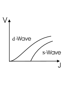
Figure 1: V versus J for s-wave and d-wave self consistency equation

As it is also clear from the figure, there is at least a region of small $J_{k}$ for which $V$ for d-wave is larger than $V$ for s-wave (in fact we can have a region with finite $V$ for d-wave but s-wave $V$ as small as we want). Now if we look at the lower band spectrum (eqn. 20 and 21) this proves that there is at least a region for small $J_{k}$ where d-wave ground state energy is lower than s-wave.

Upon moving away from half-filling, we expect that the value of ground state energy starts changing continuously; so we still have at least a region of small $J_{k}$ and small doping, for which d-wave mean-field Hamiltonian is a better approximation than s-wave. We have confirmed this by a direct numerical solution of the self-consistency equations.

IV Properties of d-wave Kondo liquid

We now study the properties of the d-wave mean-field state away from half-filling. We will see that d-wave singlet formation provides a natural route toward very anisotropic properties over the Fermi surface. Before getting into the details of these properties, we will examine some aspects of d-wave dispersion in equation 21. A schematic graph of Fermi surface for finite doping in the first Brillouin zone, as well as dispersion along a specific path, are given in figures 2 and 3 respectively. One important feature of the spectrum in figure 3 (which is also easily proved analytically in appendix A) is that the maximum value of energy in the Brillouin zone is $\mu_{f}$, that is the energy of the points along diagonal direction, where $\mu_{f}<\epsilon_{\textbf{k}}$. This shows that Fermi surface crosses the diagonal direction at a point where $E^{d}_{\textbf{k}}<\mu_{f}$ (since $E_{f}$ has to be less than $\mu_{f}$). In diagonal direction the spectrum is $E^{d}_{\textbf{k}}=\frac{\epsilon_{\textbf{k}}+\mu_{f}}{2}-|\frac{\epsilon_{\textbf{k}}-\mu_{f}}{2}|$ which can be written as:

$$\left\{\begin{array}[]{ccc}E^{d}_{\textbf{k}}=\epsilon_{\textbf{k}}&for\ \ \epsilon_{\textbf{k}}<\mu_{f}\\ E^{d}_{\textbf{k}}=\mu_{f}&for\ \ \epsilon_{\textbf{k}}>\mu_{f}\end{array}\right.$$

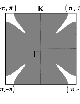
Figure 2: Fermi surface in the first Brillouin zone. Occupied region is plotted in gray.

combining this with the condition $E^{d}_{\textbf{k}}<\mu_{f}$ shows that Fermi surface should cross the diagonal direction at a point where the quasiparticles energy is equal to $\epsilon_{\textbf{k}}$. This result is in fact the basic foundation for the interesting properties that will be studied in the next sections i.e. over the Fermi surface, in diagonal direction, quasi-particles are c-electron type; the f-electron properties appear, as we go away from the diagonal direction. In the following section we will present the result of numerical calculation of properties over Fermi surface.

The self consistency equation for parameter $V$ could also be studied analytically (appendix B). We see that for d-wave Kondo model, similar to the on site s-wave Kondo, we have $V\propto e^{-\frac{C}{J_{k}}}$. Density of states at Fermi energy is also studied analytically (appendix C), it again shows exponential dependence on coupling constant:

$$\rho(E_{f})\propto V^{-2}\propto e^{\frac{2C}{J_{k}}}$$ (31)

These results were also checked and confirmed numerically.

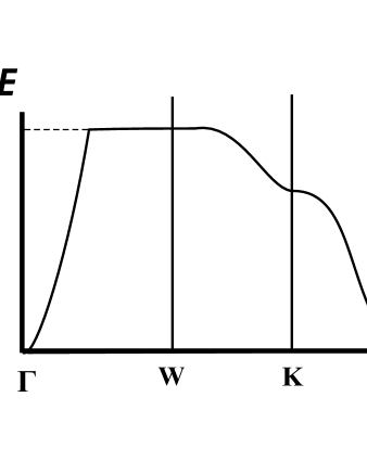
Figure 3: Spectrum along the lines $(0,0)\rightarrow(\pi,\pi)\rightarrow(0,\pi)\rightarrow(0,0)$

In the following sections we present the effective mass and quasi-particle residue on fermi surface, as a function of angle (from the center of Brillouin zone). We will see that these properties are very anisotropic as we move along the Fermi surface.

IV.1 Effective mass

The effective mass of quasi-particles is defined through second derivative of energy with respect to $k_{\perp}$ which is the momentum in direction perpendicular to Fermi surface:

$$\frac{1}{m}=\frac{\partial^{2}E^{d}_{\textbf{k}}}{\partial^{2}k_{\perp}}$$ (32)

A closed form for the effective mass could be derived. In figure 4 we have plotted the inverse effective mass over Fermi surface near diagonal direction. As we expected, along diagonal direction the effective mass matches the electron effective mass. As we go far away from the diagonal direction, effective mass becomes very large. This is because away from the diagonal direction, the quasiparticle is essentially an $f$-fermion with some weak admixture with the $c$-electron. Between these two limits we see the strange anisotropic behavior where second derivative of energy goes from electron type, positive value to large negative value. A comparison with quasi-particle residue plot (figure 6) shows that this behavior occurs where the quasi-particles are a complete mixture of $c$-electron and $f$-fermion.

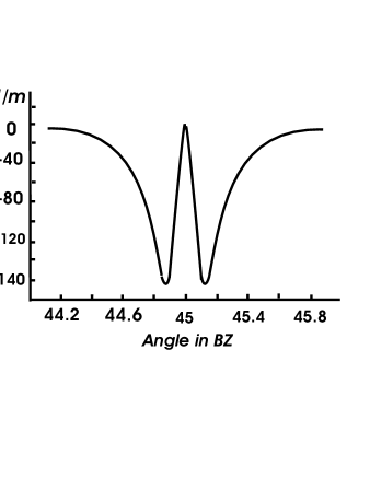
Figure 4: Second derivative of energy respect to $k_{\perp}$ in direction perpendicular to fermi surface.

This weird behavior could be traced by looking closer at the spectrum in the Brillouin zone. First consider diagonal direction (figure 5). We see that moving along this line we go from region where $E^{-}_{\textbf{k}}=\epsilon_{\textbf{k}}$ to region where $E^{-}_{\textbf{k}}=\mu_{f}$ (see figure 3). So if we plot first derivative of energy with respect to $k_{\perp}$ (which is diagonal direction for points along diagonal direction), as seen in figure 5, there is a jump from a finite value to zero at the point where $\epsilon_{\textbf{k}}=\mu_{f}$. In this direction, as shown before, at the Fermi surface $E^{-}_{\textbf{k}}=\epsilon_{\textbf{k}}$ so there is a finite value for second derivative. As we move away from diagonal direction, the jump softens slightly (because $V_{\textbf{k}}$ moves slightly from zero). But still first derivative have a large decrease in a small interval and so the second derivative is large negative number; interestingly, Fermi surface does cross this region at some points. This behavior is very strange. In fact we see points at which the effective mass is much smaller than free electron mass.

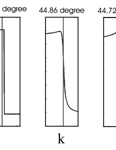
Figure 5: First derivative of the energy with respect to $k_{\perp}$. Vertical axis, in each plot, is $\frac{\partial E^{-}_{k}}{\partial k_{\perp}}\$ and $k_{\perp}$ is the momentum in direction perpendicular to the Fermi surface at the point defined by the angle on the top. Vertical line shows the position of the Fermi surface

IV.2 Quasi-particle residue

The electron-electron green function is given byMahan (1990):

$$\textit{G}(k,i\omega_{\nu})=\int_{0}^{\beta}d\tau e^{i\omega_{\nu}\tau}\langle T_{\tau}c(k,\tau)c^{\dagger}(k,0)\rangle$$ (33)

Suppose $\gamma_{\textbf{k}}^{+}$ and $\gamma_{\textbf{k}}^{-}$ are annihilation operators for quasi-particles in upper and lower bands respectively, in terms of which the Hamiltonian is diagonal. The c-electron annihilation operators could be written as:

$$\begin{split}c_{\textbf{k}}&=u_{\textbf{k}}\ \gamma_{\textbf{k}}^{+}+v_{\textbf{k}}\ \gamma_{\textbf{k}}^{-}\\ v_{\textbf{k}}^{2}&=\frac{(E^{+}_{\textbf{k}}-\epsilon_{\textbf{k}})^{2}}{(E^{+}_{\textbf{k}}-\epsilon_{\textbf{k}})^{2}+V_{\textbf{k}}^{2}}\\ u_{\textbf{k}}^{2}&=\frac{V_{\textbf{k}}^{2}}{(E^{+}_{\textbf{k}}-\epsilon_{\textbf{k}})^{2}+V_{\textbf{k}}^{2}}\\ u_{\textbf{k}}&=-\frac{V_{\textbf{k}}v_{\textbf{k}}}{E^{+}_{\textbf{k}}-\epsilon_{\textbf{k}}}\end{split}$$ (34)

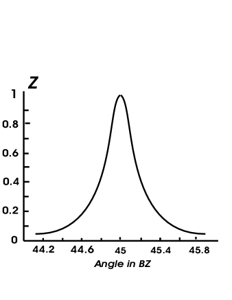
Figure 6: Quasi-particle residue on the fermi surface

Using this form (and the fact that Hamiltonian is diagonal in terms of $\gamma^{\pm}_{\textbf{k}}$ operators):

$$\langle c(\textbf{k},\tau)c^{\dagger}(\textbf{k},0)\rangle=u_{\textbf{k}}^{2}\langle\gamma^{+}_{\textbf{k}}(\tau)\gamma^{+{\dagger}}_{\textbf{k}}(0)\rangle+v_{\textbf{k}}^{2}\langle\gamma^{-}_{\textbf{k}}(\tau)\gamma^{-{\dagger}}_{\textbf{k}}(0)\rangle$$

Rewriting the Hamiltonian in term of $\gamma$ operators ($H=\sum_{\textbf{k}}(\gamma^{+{\dagger}}_{\textbf{k}}\gamma^{+}_{\textbf{k}}+\gamma^{-{\dagger}}_{\textbf{k}}\gamma^{-}_{\textbf{k}})$) we get:

$$\langle\gamma^{\pm}_{\textbf{k}}(\tau)\gamma^{\pm{\dagger}}_{\textbf{k}}(0)\rangle=e^{-E^{\pm}_{\textbf{k}}\tau}$$

Putting these into equation 33 gives:

$$\textit{G}(k,i\omega_{\nu})=\frac{u_{\textbf{k}}^{2}}{E_{\textbf{k}}^{+}-i\omega_{\nu}}+\frac{v_{\textbf{k}}^{2}}{E_{\textbf{k}}^{-}-i\omega_{\nu}}$$ (35)

By analytically continuing this to real frequencies and taking the imaginary part we get the spectral functionMahan (1990):

$$A(k,\omega)=u_{\textbf{k}}^{2}\delta(\omega-E^{+}_{\textbf{k}})+v_{\textbf{k}}^{2}\delta(\omega-E^{-}_{\textbf{k}})$$ (36)

This consists of two peaks and the weight under the low energy peak will give us the quasiparticle residue (Z). We have plotted Z for the points near diagonal direction in figure 6. Again as we expect, the quasiparticle residue near diagonal direction is of order one (electron type excitations) and gets very small away from diagonal direction.

V d-wave Kondo liquid in a Kondo-Heisenberg model: Fermi liquid with spinons

We now study the properties of the d-wave Kondo liquid state in a model which allows for explicit Heisenberg exchange interactions between the local moments. Remarkably we will show that the quasiparticle residue vanishes at isolated points of the Fermi surface in such a state. The excitation at such points is a free neutral fermionic spinon. In a subsequent Section, we show that this spinon survives even when fluctuations beyond the mean field are included. Thus this d-wave Kondo liquid is a Fermi liquid state that supports spinons at isolated Fermi points. Specifically we consider the model

$$H=\sum_{\langle ij\rangle}t_{ij}c^{\dagger}_{i}c_{j}+J_{K}\sum_{\langle ij\rangle}\vec{S}_{i}.\vec{s}_{j}+J_{H}\sum_{\langle ij\rangle}\vec{S}_{i}.\vec{S}_{j}$$ (37)

We proceed as before using the d-wave mean-field approximation to treat $\vec{S}_{i}.\vec{s}_{j}$ term; but here, we have another interacting term, which is the direct Heisenberg exchange between the local moments. Expressing this in terms of the $f$-fermions gives rise to a four fermion term. We treat this in mean field theory as well. While a number of different mean field decouplings are possible, we focus here on one in the particle-hole channel which endows the $f$-fermions with a uniform non-zero hopping $\chi$. This is in turn determined self-consistently through the equation

$$\chi=J_{H}\langle f^{\dagger}_{i}f_{j}\rangle$$ (38)

Using this, we get the following mean-field Hamiltonian:

$$\begin{split}H_{H}(k)=\sum_{k}&\epsilon_{\textbf{k}}c^{\dagger}_{\textbf{k}}c_{\textbf{k}}+\sum_{\textbf{k}}\epsilon_{f\textbf{k}}f^{\dagger}_{\textbf{k}}f_{\textbf{k}}\\ &+V\sum_{\textbf{k}}(\cos(k_{x})-\cos(k_{y}))(f^{\dagger}_{\textbf{k}}c_{\textbf{k}}+c^{\dagger}_{\textbf{k}}f_{\textbf{k}})\end{split}$$ (39)

where $\epsilon_{f\textbf{k}}=\mu_{f}-\chi\ (\cos(k_{x})+\cos(k_{y}))$. With this quadratic Hamiltonian, we can again get the spectrum:

$$\begin{split}E^{H}_{\pm}({\textbf{k}})=&\frac{\epsilon_{\textbf{k}}+\epsilon_{f\textbf{k}}}{2}\pm\\ &\sqrt{(\frac{\epsilon_{\textbf{k}}-\epsilon_{f\textbf{k}}}{2})^{2}+V^{2}(\cos(k_{x})-\cos(k_{y}))^{2}}\end{split}$$ (40)

Now let us have a closer look at this Hamiltonian and spectrum. When $V=0$, local moments and conduction electrons are not hybridized and we have two separated Fermi surfaces. The electron Fermi surface is identified by spectrum $\epsilon_{\textbf{k}}$ and is small. Spinon Fermi surface, contains one moment per site and covers half the Brillouin zoneSenthil et al. (2004).

Now assume turning on non-zero $V$. If $V$ is small enough, both bands intersect the Fermi energy. The resulting Fermi surface then consists of two sheets (each identified with one of the bands). Consider the quasi-particle residue on each band. From Eqn. 36, it is clear that on the Fermi surface of the $E^{H}_{-}$ band, quasi-particle residue is given by $v_{\textbf{k}}^{2}$ while on the other sheet (associated with $E^{H}_{+}$) it is given by $u_{\textbf{k}}^{2}$. $v_{\textbf{k}}$ and $u_{\textbf{k}}$ are defined in Eqn. 34 and satisfy

$$u_{\textbf{k}} = -\frac{V(\cos(k_{x})-\cos(k_{y}))}{E^{H}_{+}(\textbf{k})-\epsilon_{\textbf{k}}}\ v_{\textbf{k}}$$

$$u_{\textbf{k}}^{2} + v_{\textbf{k}}^{2}=1$$ (41)

Using this we see that the Fermi surface of the $-$ band has large quasiparticle residue and thus has essentially $c$-electron character (with weak admixture to $f$-fermions). On the other hand the $+$ Fermi surface has small quasiparticle residue and has essentially $f$-fermion character with weak admixture to $c$-electrons. Following reference [Senthil et al., 2004] we name the $-$ and $+$ Fermi surfaces as cold and hot surface respectively. Remarkably the quasiparticle residue on the hot Fermi surface vanishes at four isolated points (which are along the diagonal directions). At these four points the excitation is a pure $f$-fermion with no admixture to the $c$-electron. Thus at these isolated points the excitation is a neutral fermionic spinon even though spinons do not exist elsewhere on the Fermi surface.

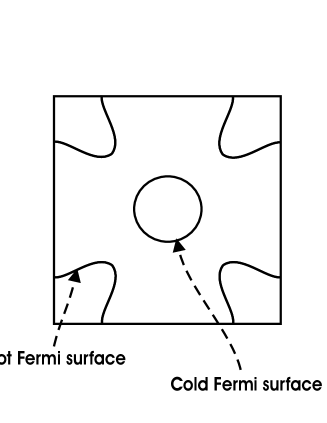
Figure 7: Fermi surface of the d-wave Kondo liquid in the Kondo-Heisenberg model

VI Quantum Hall Kondo insulators

In this Section we describe an interesting Kondo insulating state that is possible if the Kondo singlet has nontrivial internal angular momentum. Consider the generalized Kondo Hamiltonian again (12) and assume $J_{ij}$ is non-zero for nearest ($J_{1}$) and next nearest neighbors ($J_{2}$). Now, as before, we decouple the interacting term using an auxiliary field and consider the saddle point solution with nearest neighbor $V(\tau,i,j)$ the same as d-wave, and next nearest neighbor equal to $iV_{2}$ along one diagonal direction and $-iV_{2}$ along the other. Clearly this coresponds to a Kondo singlet with internal angular momentum $d_{x^{2}-y^{2}}+id_{xy}$, and describes a mean field state that spontaneously breaks time reversal symmetry. This leads to the following mean-field Hamiltonian:

$$\begin{split}H_{d+id}(\textbf{k})=\sum_{\textbf{k}}&\epsilon_{\textbf{k}}c^{\dagger}_{\textbf{k}}c_{\textbf{k}}+\sum_{\textbf{k}}\mu_{f}f^{\dagger}_{\textbf{k}}f_{\textbf{k}}\\ &+V_{1}\sum_{\textbf{k}}(\cos(k_{x})-\cos(k_{y}))(f^{\dagger}_{\textbf{k}}c_{\textbf{k}}+c^{\dagger}_{\textbf{k}}f_{\textbf{k}})\\ &+V_{2}\sum_{\textbf{k}}i\sin(k_{x})\sin(k_{y})(c^{\dagger}_{\textbf{k}}f_{\textbf{k}}-f^{\dagger}_{\textbf{k}}c_{\textbf{k}})\end{split}$$ (42)

We now specialize to a half-filled conduction band $n_{c}=1$. Diagonalizing this Hamiltonian, we readily see that the ground state in this case is a Kondo insulator with a gap. However we now show that the broken time reversal symmetry leads to a non-vanishing quantized electrical Hall conductivity. Thus this state provides an interesting example of a quantum Hall effect in a local moment system driven by the Kondo effect. To expose this physics it is convenient to rewrite the Hamiltonian in terms of a two-component fermion operator $\psi_{\textbf{k}}$:

$$\psi_{\textbf{k}}=\left(\begin{array}[]{ccc}c_{\textbf{k}}\\ f_{\textbf{k}}\end{array}\right)$$

We have

$$H=\sum_{\textbf{k}}\psi_{\textbf{k}}^{\dagger}\left(\frac{\epsilon_{\textbf{k}}+\mu_{f}}{2}+\vec{m}(\textbf{k}).\vec{\tau}\right)\psi_{\textbf{k}}$$ (43)

Here $\vec{\tau}$ are Pauli matrices operating on the two components of $\psi_{\textbf{k}}$ and $\vec{m}_{\textbf{k}}$ is a 3-dimensional vector defined in the two dimensional Brillouin zone:

$$\begin{split}\vec{m}_{\textbf{k}}=&\ \ V_{1}(\cos(k_{x})-\cos(k_{y}))\hat{x}\\ &+V_{2}\sin(k_{x})\sin(k_{y})\hat{y}\\ &+\frac{\epsilon_{\textbf{k}}-\mu_{f}}{2}\ \hat{z}\end{split}$$ (44)

Note that if $|\vec{m}|\neq 0$ over the Brillouin zone, $\vec{m}/|\vec{m}|$ is topologically a mapping from a torus (Brillouin zone) to the unite sphere. To calculate the Hall conductivity, we need the current operator. Note that in this mean field Hamiltonian, charge conservation symmetry is realized as invariance under $\psi_{\textbf{k}}\rightarrow e^{i\alpha}\psi_{\textbf{k}}$. Thus though the $f$-fermions start off as neutral, the mean field condensation of $V$ has endowed them with physical charge. This observation then leads to the current operator:

$$J_{\mu}(\textbf{k})=\frac{\partial}{k_{\mu}}H$$ (45)

We can now calculate $\sigma_{xy}$ using the Kubo formulaKubo (1957). The details of the calculation are in Appendix D. We get

$$\sigma_{xy}=\frac{e^{2}}{4\pi h}\int d^{2}k\frac{\vec{m}.(\partial_{x}\vec{m}\times\partial_{y}\vec{m})}{|\vec{m}|^{3}}$$ (46)

The value of $\sigma_{xy}$ is then invariant under smooth change of $\vec{m}$. It is thus a topological invariant of the kind considered previously by VolovikVolovik (1997). We can now change $\vec{m}$ smoothly to a mapping for which integration 46 could be calculated easily and gives twice the surface area of a unit sphere so that

$$\sigma_{xy}=\frac{2e^{2}}{h}$$ (47)

This is also confirmed with direct numerical integration. The essential physics is also simply illustrated by the following argument. As the relevant integral is a topological invariant we first imagine a smooth deformation to make $V_{2}$ infinitesimally small. In the limit when $V_{2}=0$ the gap closes and $|\vec{m}(\textbf{k})|$ has four zeroes in the Brillouin zone on the diagonal directions where $\epsilon_{\textbf{k}}=\mu_{f}$. At low energies, the physics will be dominated by modes near these nodes. On turning on a small value of $V_{2}$, we expect that the universal physics is still correctly captured, in an approximation that is legitimate for modes near the nodes. So we expand $\vec{m}(\textbf{k})$ near these nodes and take the integral over $k_{x}$ and $k_{y}$ from $-\infty$ to $\infty$. After the expansion, we get (for the node at $(k_{p},k_{p})$ in the first quadrant of the Brilloun zone):

$$\begin{split}\vec{m}_{q}=&\ \ V_{1}\sin(k_{p})\frac{q_{x}-q_{y}}{2}\hat{x}\\ &+V_{2}\sin^{2}(k_{p})\hat{y}\\ &+t\sin(k_{p})\frac{q_{x}+q_{y}}{2}\ \hat{z}\end{split}$$ (48)

Here $q_{i}=k_{i}-k_{p}$ and $\cos(k_{p})=\frac{\mu_{f}}{4t}$. After renaming $q_{x}-q_{y}$ as $k_{x}$, $q_{x}+q_{y}$ as $k_{y}$, $V_{1}\sin(k_{p})$ as $\textit{v}_{x}$, $t\sin{k_{p}}/2$ as $\textit{v}_{y}$ and $V_{2}\sin(k_{p})^{2}$ as $\Delta$, along with $90^{\circ}$ rotation of $\vec{m}$ around $x$ axis, we get the following simple form:

$$\vec{m}(\textbf{k})=\textit{v}_{x}k_{x}\hat{x}+\textit{v}_{y}k_{y}\hat{y}+\Delta\hat{z}$$ (49)

From this we trivially see that $\hat{m}(\textbf{k})=\frac{\vec{m}(\textbf{k})}{|\vec{m}(\textbf{k})|}$ points along $\hat{z}$ at $k_{x}=k_{y}=0$ and points along radial direction in $k_{x},k_{y}$ plane as $\sqrt{k_{x}^{2}+k_{y}^{2}}\rightarrow\infty$. So this vector covers half the sphere and contributes $2\pi$ to the integral in Eqn. 46. Exactly the same contribution arises from the other nodes and so we get $4\times 2\pi=8\pi$. Putting this in 46 gives the result quoted above for the electrical Hall conductivity.

Thus the $d_{x^{2}-y^{2}}+id_{xy}$ Kondo insulator has a quantized electrical Hall conductivity. A similar result - a spin and thermal quantum Hall effect - was established for two dimensional $d_{x^{2}-y^{2}}+id_{xy}$ superconductors in Ref. Senthil et al., 1999.

VII Beyond mean field theory

Through out this paper we have treated the Kondo and other interactions within the slave boson mean field theory. Now we consider the role of fluctuations beyond this mean field theory. It has been known for a long time that the important fluctuations in such mean field theories are gauge fluctuationsBaskaran and Anderson (1988). Specifically the redundant representation of the local moment spin $\vec{S}_{i}$ in terms of $f$-fermions leads to invariance of the resulting theory under local $U(1)$ gauge transformations where

$$f_{i}\rightarrow e^{i\alpha_{i}}f_{i}$$ (50)

The hybridization field in turn transforms as

$$V_{ij}\rightarrow e^{-i\alpha_{i}}V_{ij}$$ (51)

Note that the hybridization field also carries physical electric charge equal to the electron charge. As in the usual on-site slave boson theory, the mean field state is a Higgs phase where the hybridization field is condensed. Consequently the gauge fluctuations acquire a gap and can be integrated out. The Higgs condensate also implies that the $U(1)$ gauge charge of a localized $f$-fermion will be screened to produce a gauge neutral object that carries physical electric charge $1$. Thus exactly as in the usual on-site slave boson theory, the gauge fluctuations will play an innocuous role in these mean field states, and the mean field theory provides a correct qualitative description of the universal features of these phases. These considerations apply even to the $d$-wave Kondo liquid of Section V where the hybridization amplitude vanishes at four points of the ‘hot’ Fermi surface. Thus the vanishing quasiparticle residue at those four points (and the associated spinon excitations) survive beyond the mean field approximation.

VIII Discussion

The considerations of this paper may be useful in future theoretical work on a number of different correlated electron materials. The example of the cuprate materials shows that correlation effects may not uniformly affect all regions of the Fermi surface. The result is strong correlation induced anisotropy along the Fermi surface. Theoretical approaches to addressing such effects are hampered by the difficulty that correlation effects are easiest to handle in real space and not in momentum space. In this paper in the specific case of Kondo lattices, we have shown how to incorporate momentum space information into the Kondo singlet formation that determines the fate of the local moments at low temperature. We explored the properties of metallic ‘Fermi liquid’ states driven by Kondo singlet formation in a channel with non-zero internal angular momentum. Through out the paper we focused on two dimensional systems, though extension of our results to three dimensions is straightforward. We showed that such metallic states naturally have strong anisotropy of the quasiparticle effective mass and residue on moving around the Fermi surface. In some cases the quasiparticle residue even vanishes at four isolated points on the Fermi surface. The excitations at such points may be thought of as neutral spin-$1/2$ spinons that occur without any residual ‘gauge’ interactions. Thus these states provide interesting examples where strongly anisotropic quasiparticle residues are naturally built into the symmetry of the states. We also studied two dimensional Kondo insulators driven by Kondo singlet formation with complex internal angular momentum and showed that they have a quantized non-trivial electrical Hall conductivity. Such Kondo insulators thus present an interesting situation where a quantum Hall effect occurs due to the Kondo effect. Exploiting the ideas of this paper to develop techniques for thinking about the angle dependence of correlation effects in momentum space is an interesting challenge for the future.

Appendix A Maximum energy in Brillouin zone

As derived before, lower band energy at each point of Brillouin zone (BZ) is given by

$$E^{-}_{\textbf{k}}=\frac{\epsilon_{\textbf{k}}+\mu_{f}}{2}-\sqrt{(\frac{\epsilon_{\textbf{k}}-\mu_{f}}{2})^{2}+V_{\textbf{k}}^{2}}$$ (52)

where $V_{\textbf{k}}=V(\cos(k_{x})-\cos(k_{y}))$. So $V_{\textbf{k}}=0$ only along diagonal directions. From 52, we see for all points in BZ:

$$E^{-}_{\textbf{k}}\leq\frac{\epsilon_{\textbf{k}}+\mu_{f}}{2}-\sqrt{(\frac{\epsilon_{\textbf{k}}-\mu_{f}}{2})^{2}}$$ (53)

Right hand side of the above equation is equal to $\mu_{f}$ for $\mu_{f}<\epsilon_{\textbf{k}}$ and $\epsilon_{\textbf{k}}$ for $\epsilon_{\textbf{k}}<\mu_{f}$. Putting these together we get:

$$\left\{\begin{array}[]{ccc}E^{-}_{\textbf{k}}\leq\epsilon_{\textbf{k}}&for\ \ \epsilon_{\textbf{k}}\leq\mu_{f}\\ E^{-}_{\textbf{k}}\leq\mu_{f}&for\ \ \epsilon_{\textbf{k}}>\mu_{f}\end{array}\right.$$ (54)

You see that all points in BZ, obviously, satisfy one the two conditions ($\epsilon_{\textbf{k}}\leq\mu_{f}$ or $\epsilon_{\textbf{k}}>\mu_{f}$). So we get for any point in the BZ:

$$E^{-}_{\textbf{k}}\leq\mu_{f}$$ (55)

A closer look at equations 52 and 53, shows that equality in equation 55, could be only for the points along diagonal direction with $\epsilon_{\textbf{k}}>\mu_{f}$. Such points cover a region with zero volume in the BZ. So that for any finite doping $E_{f}<\mu_{f}$ (see section IV).

Appendix B Self consistency equation

Analytic treatment of self consistency relation is easier and much more clear at zero doping ($\mu_{f}=0$). So we start with this case and later, we can argue if our result might be modified at finite, but small, doping. In continuum limit, self consistency relation (at zero doping) have the form:

$$\frac{1}{J_{k}}=\frac{1}{2n}\int\frac{d^{2}k}{(2\pi)^{2}}\frac{(\cos(k_{x})-\cos(k_{y}))^{2}}{\sqrt{(\frac{\epsilon_{\textbf{k}}}{2})^{2}+V^{2}(\cos(k_{x})-\cos(k_{y}))^{2}}}$$ (56)

where $n$ is density of lattice sites. We saw before that, this equation for $V$ has a solution, no matter how small $J_{k}$ is (see section LABEL:lecomp). This was because, the integral is divergent at $V=0$. The divergence comes from the region where $\epsilon_{\textbf{k}}$ is small. So to study the behavior of this integral, it is enough to look at the points where $\epsilon_{\textbf{k}}$ is small. Because of the symmetry of BZ with respect to $90^{\circ}$ rotation, it is enough to consider region with $k_{x},k_{y}\geq 0$. The point with $\epsilon_{\textbf{k}}=0$ in this region, are points with $k_{x}=\pi-k_{y}$. We want to look around such points so if we change the variables to $k_{y}\rightarrow k_{y}$ and $k_{x}\rightarrow q=k_{y}+k_{x}-\pi$, we just want to look at region with small $q$. Putting these variables in to in to 56 and expanding up to first non-zero order in $q$, we get:

$$\begin{split}\frac{1}{J_{k}}=\frac{1}{2n}\int&\frac{dk_{y}dq}{(2\pi)^{2}}\\ &\frac{(\sin(k_{y})q+2\cos(k_{y}))^{2}}{\sqrt{(t\sin(k_{y})q)^{2}+V^{2}(\sin(k_{y})q+2\cos(k_{y}))^{2}}}\end{split}$$ (57)

As discussed before, we like to study the singular behavior around $q=0$ so we can ignore the $q$ dependence in non-singular terms. The relation simplifies to:

$$\frac{1}{J_{k}}=\frac{1}{2n}\int\frac{dk_{y}dq}{(2\pi)^{2}}\frac{(2\cos(k_{y}))^{2}}{\sqrt{(t\sin(k_{y})q)^{2}+V^{2}(2\cos(k_{y}))^{2}}}$$ (58)

Now we first perform the integral over $k_{y}$. Note that the limits for this is $q$ dependent (i.e. $0+O(q^{2})$ and $\pi+O(q^{2})$) but these also could be ignored since they have no effect on singular behavior:

$$\frac{1}{J_{k}}=\frac{1}{2n}\int\frac{dq}{2\pi}\int_{0}^{\pi}\frac{dk_{y}}{(2\pi)}\frac{(2\cos(k_{y}))^{2}}{\sqrt{(t\sin(k_{y})q)^{2}+V^{2}(2\cos(k_{y}))^{2}}}$$ (59)

Integral over $k_{y}$ could be perform exactly which gives:

$$\frac{2}{|q|}\ _{2}F_{1}(\frac{1}{2},\frac{3}{2};2;1-\frac{V^{2}}{q^{2}})$$ (60)

here, $\-{}_{2}F_{1}$ is Hypergeometric Function. We are in interested in small $q$ behavior so $1-\frac{V^{2}}{q^{2}}\approx-\frac{V^{2}}{q^{2}}$. The expression could be simplified using the identityOberhettinger (1972):

$$\ {}_{2}F_{1}(a,b;c;z)=(1-z)^{-a}\ _{2}F_{1}(a,c-b;c;\frac{z}{z-1})$$

Using this for the result of integral we get:

$$\frac{1}{J_{k}}\approx\frac{1}{2n}\int\frac{dq}{2\pi}\frac{2}{\sqrt{q^{2}+V^{2}}}\ _{2}F_{1}(\frac{1}{2},\frac{1}{2};2;1)$$ (61)

where we used the fact $\frac{-\frac{V^{2}}{q^{2}}}{-\frac{V^{2}}{q^{2}}-1}\approx 1$. Since ${}_{2}F_{1}(\frac{1}{2},\frac{1}{2};2;1)$ is convergentOberhettinger (1972) we get:

$$\frac{1}{J_{k}}=A\int\frac{dq}{\sqrt{q^{2}+V^{2}}}$$ (62)

where $A$ is a finite constant. Integral over $q$ is now trivial and leads to result mentioned before (see section IV):

$$V\propto e^{-\frac{C}{J_{k}}}$$ (63)

After dopinping, continuum form of self consistency relation changes:

$$\begin{split}\frac{1}{J_{k}}=\frac{1}{2n}\int\frac{d^{2}k}{(2\pi)^{2}}&\ \Theta(E_{f}-E^{-}\textbf{k})\\ &\frac{(\cos(k_{x})-\cos(k_{y}))^{2}}{\sqrt{(\frac{\epsilon_{\textbf{k}}-\mu_{f}}{2})^{2}+V^{2}(\cos(k_{x})-\cos(k_{y}))^{2}}}\end{split}$$ (64)

Again dominant contribution comes from the region where $|\epsilon_{\textbf{k}}-\mu_{f}|$ is small. Similar expansion could be carried out but this time the points we look at are close to different curve (defined by $\cos(k_{x})+\cos(k_{y})=\frac{\mu_{f}}{2t}$ which is slightly away from $k_{x}=\pi-k_{y}$ for small $\mu_{f}$). We don’t expect (and in fact the resulting integral shows) that there is not much change in singular behavior as $V$ goes to zero. So we expect that behavior seen in 63 holds and in fact this is confirmed with numerical studies.

Appendix C Density of states

To get density of states we use the general formulaAshcroft and Mermin (1976):

$$\rho(E_{f})=\int\frac{d^{2}k}{(2\pi)^{2}}\ \delta(E_{f}-E^{-}_{\textbf{k}})$$ (65)

Again symmetries in BZ are helpful. First of all we can do the calculation on one patch of Fermi surface (in $k_{x}\leq 0$ and $k_{y}\leq 0$ quarter). Also because of reflection symmetry respect to diagonal, we can do the calculation for the points on Fermi surface which are above the diagonal and double the result. Now in this region we can safely (since $\epsilon_{\textbf{k}}$ is one to one function of $(k_{x},k_{y})$) do the change of variable, and work with $k_{y}$ and $\epsilon_{\textbf{k}}$:

$$\rho(E_{f})=\int\frac{dk_{y}}{(2\pi)^{2}}\frac{d\epsilon_{\textbf{k}}}{2t\sqrt{1-(\frac{\epsilon_{\textbf{k}}}{2t}-\cos(k_{y}))^{2}}}\ \delta(E_{f}-E^{-}_{\textbf{k}})$$ (66)

Note that $\sqrt{1-(\frac{\epsilon_{\textbf{k}}}{2t}-\cos(k_{y}))^{2}}=\sin(k_{x})$ is never zero in the part of BZ we are integrating over. In terms of new variables:

$$E^{-}_{\textbf{k}}=\frac{\epsilon_{\textbf{k}}+\mu_{f}}{2}-\sqrt{(\frac{\epsilon_{\textbf{k}}-\mu_{f}}{2})^{2}+V^{2}(\frac{\epsilon_{\textbf{k}}}{2t}-2\cos(k_{y}))^{2}}$$ (67)

Using this we first do the integration over $\epsilon_{\textbf{k}}$ which leads to:

$$\begin{split}\rho(E_{f})=\int&\frac{dk_{y}}{(2\pi)^{2}}\frac{1}{2t\sqrt{1-(\frac{\epsilon}{2t}-\cos(k_{y}))^{2}}}\\ &\left(\frac{1}{2}-\frac{\frac{\epsilon-\mu_{f}}{4}+(V^{2}/2t)(\frac{\epsilon}{2t}-2\cos(k_{y}))}{\sqrt{(\frac{\epsilon-\mu_{f}}{2})^{2}+V^{2}(\frac{\epsilon_{\textbf{k}}}{2t}-2\cos(k_{y}))^{2}}}\right)^{-1}\end{split}$$ (68)

here, $\epsilon$ is solution of equation:

$$E_{\textbf{k}}^{-}=E_{f}$$

for $\epsilon_{\textbf{k}}$, which is a simple second order equation but we avoid presenting the answer which is not necessary for the rest of calculation. Now to proceed we need to divide to points in three different regions. The first region is defined by the points where:

$$(\frac{\epsilon_{\textbf{k}}-\mu_{f}}{2})^{2}\sim V^{2}(\frac{\epsilon_{\textbf{k}}}{2t}-2\cos(k_{y}))^{2}$$

for these points contribution to 68 is of order one.

The other regions are where:

$$(\frac{\epsilon_{\textbf{k}}-\mu_{f}}{2})^{2}\gg V^{2}(\frac{\epsilon_{\textbf{k}}}{2t}-2\cos(k_{y}))^{2}$$ (69)

This contains most of the points on the Fermi surface, since from 63 we know that $V$ is small. Now we expand expression in prentices in 68 up to first non-zero order in $V^{2}$:

$$\rho(E_{f})=\int\frac{dk_{y}}{(2\pi)^{2}}\left(\frac{1}{2}(1-Sign(\epsilon_{\textbf{k}}-\mu_{f}))+\frac{V^{2}}{t^{2}}f(\epsilon,k_{y})\right)^{-1}$$ (70)

here $f(\epsilon,k_{y})$ is convergent function. We don’t need the detailed form of this function though. The important property of this integral is that for points with $\epsilon_{\textbf{k}}<\mu_{f}$ (which corresponds to points near diagonal as discussed in A) contribution to integral is of order one. We expected this since in this region quasi-particles are more free electron like. However for points with $\epsilon_{\textbf{k}}>\mu_{f}$ (which are away from diagonal) contribution is large and proportional to $V^{-2}$. Putting all these together we get a large density of state:

$$\rho(E_{f})\propto e^{\frac{2C}{J_{k}}}$$ (71)

Appendix D Kubo calculation

Using equation 45 we can write $J_{\mu}$ as:

$$J_{\mu}(\tau)=\sum_{\textbf{k}}\psi^{\dagger}(\tau)(\partial_{\mu}a(\textbf{k})+\partial_{\mu}\vec{m(\textbf{k})}.\vec{\sigma})\psi(\tau)$$ (72)

where $\vec{m(\textbf{k})}$ is defined in 44 and $a(\textbf{k})=\frac{\epsilon_{\textbf{k}}+\mu_{f}}{2}$. Also $\partial_{\mu}$ is the shorthand for $\frac{\partial}{\partial k_{\mu}}$. Putting this form in Kubo formulaKubo (1957) we get:

$$\begin{split}\sigma_{\mu\nu}(\omega)=\int d\tau&\frac{e^{-i\omega\tau}-1}{\omega}\times\\ \sum_{k,k^{\prime}}\langle&\psi^{\dagger}(\tau)(\partial_{\mu}a(\textbf{k})+\partial_{\mu}\vec{m}(\textbf{k}).\vec{\sigma})\psi(\tau)\\ \ \ &\psi^{\dagger}(0)(\partial_{\nu}a(k^{\prime})+\partial_{\nu}\vec{m}(k^{\prime}).\vec{\sigma})\psi(0)\rangle\end{split}$$ (73)

Using the Hamiltonian given in 43 we get the green function for $\psi$ fields:

$$G(i\omega,k)=\frac{1}{i\omega-a(\textbf{k})-\vec{m}(\textbf{k}).\vec{\sigma}}$$ (74)

With this in hand, the Kubo equation reduces to the following form:

$$\begin{split}&\omega\sigma_{xy}(\omega)=\sum_{\textbf{k}}\int\frac{dE}{2\pi}\\ &tr\left[\frac{(\partial_{x}a(\textbf{k})+\partial_{x}\vec{m}(\textbf{k}).\vec{\sigma})(\partial_{y}a(\textbf{k})+\partial_{y}\vec{m}(\textbf{k}).\vec{\sigma})}{(iE-a(\textbf{k})-\vec{m}(\textbf{k}).\vec{\sigma})}\right.\times\\ &\left.\left(\frac{1}{(i(\omega+E)-a(\textbf{k})-\vec{m}(\textbf{k}).\vec{\sigma})}-\frac{1}{(iE-a(\textbf{k})-\vec{m}(\textbf{k}).\vec{\sigma})}\right)\right]\end{split}$$ (75)

We are interested in the limit of above equation as $\omega\rightarrow 0$. In this limit we get the following expression for Hall conductivity:

$$\begin{split}\sigma_{xy}=&-i\int\frac{d^{2}k}{(2\pi)^{2}}\frac{dE}{2\pi}\\ &tr\left[(\partial_{x}a(\textbf{k})+\partial_{x}\vec{m}(\textbf{k}).\vec{\sigma})\frac{1}{(iE-a(\textbf{k})-\vec{m}(\textbf{k}).\vec{\sigma})^{2}}\right.\\ &\left.(\partial_{y}a(\textbf{k})+\partial_{y}\vec{m}(\textbf{k}).\vec{\sigma})\frac{1}{(iE-a(\textbf{k})-\vec{m}(\textbf{k}).\vec{\sigma})}\right]\end{split}$$ (76)

Expanding out the sums, we have several terms but taking the trace, cancel some of the terms. After integration over the $E$ and dropping the terms which are zero under the trace gives:

$$\begin{split}\sigma_{xy}=-i\int\frac{d^{2}k}{(2\pi)^{2}}&\frac{1}{8|\vec{m}(\textbf{k})|^{3}}\\ &tr\left(\partial_{x}\vec{m}(\textbf{k})\right.\left.[\vec{m}(\textbf{k}).\vec{\sigma},\partial_{y}a(\textbf{k})+\partial_{y}\vec{m}(\textbf{k}).\vec{\sigma}]\right)\end{split}$$ (77)

After doing some algebra on the Pauli matrices and taking the trace, we get the relation given in 46.

References

- Kondo (1966) J. Kondo, Progr. Theoret. Phys. (Kyoto) 36, 429 (1966).
- Doniach (1977) S. Doniach, Physica B 91, 231 (1977).
- Luttinger (1960) J. M. Luttinger, Phys. Rev. 119, 1153 (1960).
- Nozieres (1998) P. Nozieres, Eur. Phys. B 6, 447 (1998).
- Read and Sachdev (1991) N. Read and S. Sachdev, Phys. Rev. Lett. 66, 1773 (1991).
- Wen (1991) X.-G. Wen, Phys. Rev. B 44, 2664 (1991).
- Senthil and Fisher (2000) T. Senthil and M. P. A. Fisher, Phys. Rev. B 62, 7850 (2000).
- Ribeiro and Wen (2005) T. C. Ribeiro and X.-G. Wen, Phys. Rev. lett. 95, 057001 (2005).
- Lee et al. (2006) P. A. Lee, N. Nagaosa, and X.-G. Wen, Rev. Mod. Phys. 78, 17 (2006).
- Zhou et al. (2004) X. J. Zhou, T. Yoshida, D.-H. Lee, W. Yang, V. Brouet, F. Zhou, W. Ti, J. Xiong, Z. X. Zhao, T. Sasagawa, et al., Phys. Rev. Lett. 92, 187001 (2004).
- Civelli et al. (2005) M. Civelli, M. Capone, S. S. Kancharla, O. Parcollet, and G. Kotliar, Phys. Rev. Lett. 95, 106402 (2005).
- Read et al. (1984) N. Read, D. Newns, and S. Doniach, Phys. Rev. B 630, 3841 (1984).
- Millis and Lee (1987) A. Millis and P. Lee, Phys. Rev. B 35, 3394 (1987).
- Moreno and Coleman (2000) J. Moreno and P. Coleman, Phys. Rev. Lett. 84, 342 (2000).
- Burch et al. (a) K. S. Burch, S. V. Dordevic, F. P. Mena, D. van del Marel, J. L. Sarrao, J. R. Jeffries, E. D. Bauer, M. B. Maple, and D. N. Basov, eprint cond-mat/0604146.
- Burch et al. (b) K. S. Burch, S. V. Dordevic, F. P. Mena, A. B. Kuzmenko, D. van del Marel, J. L. Sarrao, J. R. Jeffries, E. D. Bauer, M. B. Maple, and D. N. Basov, eprint unpublished.
- Coleman (2002) P. Coleman, Lectures on the Physics of Highly Correlated Electron Systems VI (American Institute of Physics, 2002), p. 97, edited by: F. Mancini.
- Mahan (1990) G. D. Mahan, Many-Particle Physics (Plenum Press, 1990).
- Senthil et al. (2004) T. Senthil, M. Vojta, and S. Sachdev, Phys. Rev. B 69, 035111 (2004).
- Kubo (1957) R. Kubo, J. Phys. Soc. Jpn. 12, 570 (1957).
- Volovik (1997) G. E. Volovik, Pis’ma ZhETF 66, 492 (1997).
- Senthil et al. (1999) T. Senthil, J. B. Marston, and M. P. A. Fisher, Phys. Rev. B 60, 4245 (1999).
- Baskaran and Anderson (1988) G. Baskaran and P. W. Anderson, Phys. Rev. B 37, 580 (1988).
- Oberhettinger (1972) F. Oberhettinger, Handbook of Mathematical Functions with Formulas, Graphs, and Mathematical Tables (Dover, 1972), p. 555, edited by: Milton Abramowitz and Irene A. Stegun.
- Ashcroft and Mermin (1976) N. W. Ashcroft and N. D. Mermin, Solid State Physics (Saunders College Publishing, 1976).