Linear response in aging glassy systems, intermittency and the Poisson statistics of record fluctuations.

Abstract

We study the intermittent behavior of the energy decay and linear magnetic response of a glassy system during isothermal aging after a deep thermal quench using the Edward-Anderson spin glass model as a paradigmatic example. The large intermittent changes in the two observables are found to occur in a correlated fashion and through irreversible bursts, ‘quakes’, which punctuate reversible and equilibrium-like fluctuations of zero average. The temporal distribution of the quakes it foun to be a Poisson distribution with an average growing logarithmically on time, indicating that the quakes are triggered by record sized fluctuations. As the drift of an aging system is to a good approximation subordinated to the quakes, simple analytical expressions (Sibani et al. Phys Rev B 74, 224407, 2006) are available for the time and age dependence of the average response and average energy. These expressions are shown to capture the time dependencies of the EA simulation results. Finally, we argue that whenever the changes of the linear response function and of its conjugate autocorrelation function follow from the same intermittent events a fluctuation-dissipation-like relation can arise between the two in off-equilibrium aging.

1 Motivation

In noise spectra from mesoscopic aging systems, reversible fluctuations are punctuated by rare and large, so called intermittent, events Kegel00 ; Weeks00 ; Bissig03 ; Buisson03 ; Buisson04 ; Cipelletti05 , which arguably signal switches from one metastable configuration to another Crisanti04 ; Sibani05 . The intermittent events usually appear as an exponential tail in the Probability Density Function (PDF) of the fluctuations. The central part of the PDF describes equilibrium-like behavior with its zero-centered Gaussian shape. Exploiting this information can adds new twists to long debated issues as the multiscale nature of glassy dynamics and the associated memory behavior.

A record dynamics scenario for aging Sibani05 ; Sibani93a ; Sibani03 builds on two main assumptions: (i) record sized energy fluctuations within metastable domains trigger irreversible intermittent events, or quakes; (ii) these, in turn, control all significant physical changes, e.g. heat release, configurational decorrelation and linear magnetic response. In brief, all important changes are considered to be subordinated to the quakes, with the latter triggered by energy fluctuations of record size. Combining the information from the equilibrium-like fluctuations with non-thermal properties, e.g. irreversible energy losses, leads to testable predictions for the time and temperature dependencies of the fluctuation spectra which have been confirmed in a number of cases Sibani05 ; Anderson04 ; Sibani04a ; Sibani06 ; Oliveira05 ; Sibani06b ; Sibani06a .

$\begin{array}[]{cc}\includegraphics[width=203.80193pt,height=203.80193pt]{dMPDF.eps}&\includegraphics[width=203.80193pt,height=203.80193pt]{dEPDF.eps}\end{array}$

Figure 1: (Color on line) The left panel shows the PDF (blue circles) of the magnetization changes $\delta M$ occurring over intervals of length $\delta t=20$ during isothermal simulations at temperature $T=0.4$. The statistics is based on $2\cdot 10^{5}$ data points obtained in the age interval $[1000,3000]$ using $2000$ independent trajectories. The zero average Gaussian (black line) fits data points with $-80<\delta M<50$. The right panel shows the PDF of the energy changes (blue circles), and a Gaussian fit of the positive energy fluctuations (black line). The red squares pertain to the subset of energy changes occurring in the immediate vicinity of large ($\delta M>50$ ) magnetization changes. All data are obtained from the same set of trajectories as those shown in the left panel.

While macroscopic (average) linear response functions have long been the tool of choice for probing aging in magnetic systems, Lundgren83 ; Alba86 ; Zotev03 ; Rodriguez03 ; Suzuki03 , the predictions of record dynamics have so far only been tested for experimental Thermoremanent Magnetization (TRM) data. spin glass data Sibani06a . Simulations offer certain advantages over experiments: it is possible to simulate an instantaneous quench, simply by choosing a ‘random’, i.e. high temperature, initial condition. Notably, an instantaneous initial quench leads to the ‘full aging’ Rodriguez03 , scaling behavior simply explained in record dynamics; secondly, the statistical analysis is considerably simplified when thousands of independent traces can be generated; lastly, temporal correlations between the intermittent changes of the magnetization and the energy can be extracted.

The Edwards-Anderson (EA) spin-glass model used in this work is a paradigmatic example of an aging system. Its macroscopic (average) magnetic response and autocorrelation decay have been thoroughly investigated Andersson92 ; Rieger93 ; Kisker96 ; Picco01 and its mesoscopic fluctuations properties have attracted some recent attention Castillo03 ; Sibani05 ; Sibani06 . Here, data from extensive simulations are analyzed with focus on the intermittency of the energy and Zero Field Cooled Magnetization (ZFCM) fluctuations We confirm that quakes carry the net drift of the energy Sibani05 and correlate strongly with the large intermittent magnetization fluctuations carrying the net change of the linear response. The idea Sibani03 ; Sibani05 that quakes have a Poisson distribution with a logarithmic time dependence is derived from record statistics and is central to the theory. To verify it empirically, we consider the temporal statistics of the difference of ’logarithmic waiting times’ $\log(t_{q})-\log(t_{q-1})$, where $t_{q}$ marks the occurence of the $q$’th quake in a given trace. For the above Poisson distribution, these logarithmic differences are exponentially distributed. General mathematical arguments lead to eigenvalue expansions for the dependence of the average energy and linear response on the number of quakes, and then, via the subordination hypothesis, to power-law expansions for the time dependences of the same quantities Sibani06 ; Sibani06a . The expansions are tested below against the EA model numerical simulation results. The origin of approximate off-equilibrium Fluctuation-Dissipation like relations is discussed in the last section from the point of view of record dynamics.

Finally, a notational issue: as in ref. Sibani06a , the variable $t$ generically denotes the time elapsed from the initial quench, i.e. the system age. The external field is switched on at time $t=t_{w}$, and $t_{obs}=t-t_{w}$ denotes the observation time, a quantity called $t$ in refs. Sibani05 ; Sibani06 and in many experimental papers e.g.  Vincent96 ; Rodriguez03 . Unless otherwise stated, we denote the average energy and magnetization by $\mu_{e}$ and $\mu_{ZFCM}$, and reserve the symbols $e$ and $M$ for the corresponding fluctuating quantities measured in the simulations. The simulation temperature is denoted by $T$.

2 Model and Simulation methods

$\begin{array}[]{cc}\includegraphics[width=203.80193pt,height=203.80193pt]{pdfs.eps}&\includegraphics[width=203.80193pt,height=203.80193pt]{gaussian_var.eps}\end{array}$

Figure 2: (Color on line) The left panel depicts the PDF of the magnetization changes $\delta M$ over intervals of length $\delta t$. The simulation temperature is $T=0.4$. Green circles, blue squares and magenta diamonds correspond to $\delta t=20,40$ and $60$, respectively. The data are collected in the interval $[1000,3000]$. In order of increasing $\delta t$, the statistics is based on $10^{5}$, $.5\cdot 10^{5}$ and $.33\cdot 10^{5}$ data points. The full line is a fit of all data with $-80<\delta M<50$ to a Gaussian centered at zero. For $\delta M>50$ the PDF clearly deviates from a Gaussian shape. The intermittent tail grows with $\delta t$ and fully determines the average change in the ZFC magnetization. The insert shows $dM$, averaged over $t_{obs}$, versus $\delta t$. The right panel shows the variance of the (fitted) Gaussians as a function of the reduced temperature $T/T_{g}$.

In the Edwards-Anderson model, $N$ Ising variables, $\sigma_{i}=\pm 1$, are placed on a cubic lattice with toroidal boundary conditions. Their interaction energy is

$$E=-\frac{1}{2}\sum_{i,j}^{N}\sigma_{i}\sigma_{j}J_{ij}-H\sum_{i}^{N}\sigma_{i},$$ (1)

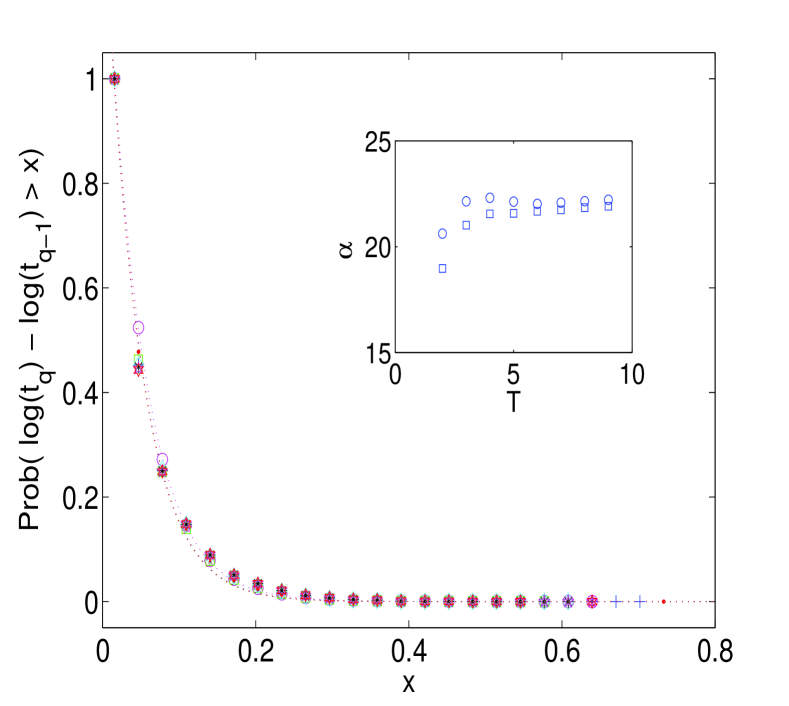
Figure 3: (Color on line) For eight different temperatures $T=0.2,0.3\ldots 0.9$ (circles, dots, squares, plusses, diamonds,stars, pentagrams, and hexagrams) the estimated cumulative probability Prob$(\log t_{q}/t_{q-1}>x)$ is plotted versus $x$, with $t_{q}$, $q=1,2\ldots$ denoting the times at which the quakes occur. The quakes are identified as described in the main text using the filtering parameter value $f=7$. The dotted lines are fits to the exponential $\exp(-\alpha x)$. The collapse of the eight data sets demonstrates that the temperature dependence is very weak, except at the lowest $T$. In the insert, the fitted $\alpha$ values are plotted versus $T$. The circles pertain to the data shown in the main plot, and the squares pertain to corresponding data obtained using $f=8$ as a filter parameter.

where $\sum_{i}\sigma_{i}=M$ is the magnetization and $H$ is the magnetic field. The non-zero elements of the symmetric interaction matrix $J_{ij}$ connect neighboring sites on the lattice. The interactions are drawn from a Gaussian distribution with zero average and unit variance, a choice setting the scale for both temperature and magnetic field.

In the simulations, we use system size $N=16^{3}$ and collect the statistics of energy and magnetization changes from either several thousands of independent trajectories, each corresponding to a different realization of the $J_{ij}$’s. After the initial quench, aging procedes isothermally in zero field untill time $t=t_{w}$, where a small magnetic field $H=0.1$ is instantaneously turned on. Isothermal simulations lasting up to age $t=100\,t_{w}$ are carried out for $t_{w}=50,100,200,500$ and $1000$ at temperatures $T=0.1,0.2,\ldots 0.8$. The simulation engine utilizes the Waiting Time Method Dall01 ; Sibani06b , a rejectionless or ‘event driven’ algorithm which operates with an ‘intrinsic’ time, loosely corresponding to a sweep of the Metropolis algorithm. Unlike the Metropolis algorithm, the WTM can follow spatio-temporal patterns on very short time scales, a property advantageous for intermittency studies.

3 Simulation results

In this Section, simulation results are presented together with some relevant theoretical considerations. The first subsection deals with the distribution of energy and magnetization changes, $\delta E$ and $\delta M$, occurring over small intervals $\delta t$. The Probability Density Function (PDF) of these quantities characterizes intermittency in the EA model in a simple and direct way. In the second subsection, the quakes are (approximately) indentified within each data stream, and the temporal aspects of their distribution are studied. In the third and last subsection, the average linear response and average energy obtained from the simulations are compared to analytical predictions which are based on the temporal distribution of the quakes.

3.1 Energy and magnetization fluctuation statistics

For a first statistical description of the energy and the ZFCM fluctuations, energy and magnetization changes $\delta E$ and $\delta M$ occurring over small intervals $\delta t$ are sampled during the time interval $[1000,3000]$. The left panel of Fig. 1 shows the PDF of the magnetic fluctuations (blue circles) on a log scale. The (black) line is the fit to a zero-centered Gaussian obtained using data within the interval $-80<\delta M<50$. The distribution of the remaining large positive magnetization changes is seen to have exponential character. The same runs are used to collect the PDF of the energy fluctuations, shown in the right panel of Fig. 1 (lower data set, blue circles). Again, we see a combination of a zero centered Gaussian and an intermittent exponential tail. The full line is a fit to the zero centered Gaussian in the interval $-5<\delta E<20$.

As intermittent fluctuations are rare, the temporal correlation between intermittent energy and ZFC magnetization changes is best observed using conditional PDF’s (upper curve, red squares). The conditional PDF shown only includes those $\delta E$ values which either fall in the same or in the preceding small interval of width $\delta t$ as magnetic fluctuations above the threshold $\delta M=50$. In the left panel of the figure, the threshold is seen to be near the boundary between reversible and intermittent magnetization changes. Note how the Gaussian parts of the full and of the conditional PDFs nearly coincide, while the corresponding intermittent tails differ. The tail of the conditional PDF is strongly enhanced (roughly, between $10$ and $100$ times) when only fluctuations near a large magnetization change are included in the count. A similar situation is observed at any low temperatures.

Figure 2 details the dependence of the PDF of the magnetization fluctuations on $\delta t$ and $T$: The three PDFs shown in the left panel of Fig. 2 as green circles, blue squares and magenta diamonds are obtained in the interval $[1000,3000]$, for $T=0.4$ and for $\delta t=20,40$ and $60$, respectively. The black line is a zero centered Gaussian fitted to the PDF in the range $-80<\delta M<10$. The fit is obtained by optimizing the variance of the Gaussian distribution, $\sigma_{G}^{2}$. The latter quantity should not be confused with the variance of the full distribution, which is much larger and heavily influenced by the tail events excluded from the Gaussian fit. Importantly, since the Gaussian part of the PDF is independent of $\delta t$ quasi-equilibrium ZFCM fluctuations at $T=0.4$ can be treated as uncorrelated for times larger than $\delta t=20$. Secondly, since the Gaussian is centered at zero, any changes in the average magnetization are exclusively due to the intermittent events. Similar conclusions were reached for the spin-glass TRM magnetization, Sibani06a and for the energy outflow in the EA model, Sibani05 and in a p-spin model with no quenched randomness. Sibani06b The insert describes the dependence on $\delta t$ of the magnetization change $\langle\delta M\rangle$ averaged over the observation interval $[1000,3000]$. E.g. the data point corresponding to $\delta t=20$ depicts the average of the lowest PDF plotted in the main figure. The right panel of fig. 2 shows a plot of the ratio $\sigma^{2}_{G}/T$ versus $T$ for the Gaussian part of the magnetic fluctuations. As the Fluctuation-Dissipation Theorem (FDT) applies to the equilibrium-like part of the dynamics, the ordinate can be interpreted as the (gedanken) linear magnetic susceptibility of metastable configurations. The overall shape of the curve is reminiscent of the experimental $T$ dependence of the ZFCM below $T_{g}$. Nordblad87

3.2 Temporal distribution of intermittent events

The PDF of intermittent fluctuations in the EA model scales with the ratio $\delta t/t$, where $t$ is the age of the system at the beginning of the sampling interval Sibani05 . The rate of quakes accordingly decays as the inverse of the age, in agreement with the claim that the the number of independent quakes in an interval $(t,t^{\prime})$ has a Poisson distribution with average $\langle n_{I}\rangle=\alpha\log(t/t^{\prime})$ The parameter $\alpha$ characterizing the average is interpreted as the number of thermalized domains contributing in parallel to the fluctuation statistics. This quantity is expected to be temperature independent and linearly dependent on system size Sibani06b . Using that the differences $\tau_{q}=\log(t_{q})-\log(t_{q-1})=\log(t_{q}/t_{q-1})$ are independent random numbers, all exponentially distributed with the same average $\langle\tau_{q}\rangle=1/\alpha$, identifying the times $t_{q}$, $q=1,2,\ldots$ at which the quakes occur allows one to check the temporal aspects of statistics (as opposed to the distributionof quake sizes).

The identification entails some challanges of statistical and patter-recognition nature. The residence times $t_{q}-t_{q-1}$ expectedly have a broad distribution Sibani03 , which, in connection with a finite sampling time creates a negative sampling bias on large $t_{q}$ values Anderson04 , even with the quakes unabiguously identified. Secondly, correlations may well be present between large and closely spaced spikes in the signal which collectively represent a change of attractor. Last but not least, identification of the $t_{q}$’s within a trace must rely on the negative sign of the fluctuations and on their ’sufficiently large’ size. I.e. by definition sufficient energy must be released to make the reverse process highly unprobable within an observation span stretching up to $2t$ for a quake which occurs at $t$. Sibani03 A related and generic property of aging systems (also directly accessible by an intermittency analysis Sibani05 ) is that reversible equilibrium-like fluctuations dominate the dynamics on time scales shorter than the age $t$. A simple empirical criterion for distinguishing reversible fluctuations from irreversible quakes uses an upper bound on the probability, $P_{rev}(t,\delta E)$ that at least one thermal energy fluctuation of positive sign be among the $t/\delta t$ observations. For small $\exp(-\delta E/T)$, this happens with probability $P_{rev}(t,\delta E)\approx t/\delta tc\exp(-\delta E/T)$, where the positive number $c$ is unknown. A negative energy fluctuation is labeled as a quake if its absolute value $|\delta E|$ satisfies $P_{rev}(t,|\delta E|)<10^{-n}$, where $n$ is a positive number. For a thermal fluctuation which occurs at age $t$, this criterion produces the inequality

$$\frac{|\delta E|_{\rm quake}}{T}>f+\log t;\quad\mbox{\rm where}\quad f=n\ln(10)+\ln(c/\delta t).$$ (2)

The formal definition of the ‘filter’ parameter $f$ on the right hand side of the inequality contains the unknown parameter $c$ as well as a free parameter $n$. We must therefore treat $f$ as a free parameter regulating how strict a filter the fluctuations must pass to qualify as quakes.

For temperatures $T=0.2,0.3\ldots 0.9$, a range spanning most of the EA spin-glass phase, simulations were performed in the interval $t\in(200,10200)$. Within each trajectory, quakes are identified by applying Eq. 2, and the quantities $\tau_{q}=\log(t_{q}/t_{q-1})$ are calculated and binned. The procedure is repeated for $2000$ independent trajectories for each value of the temperature. The magnetic field values $H=0.1$ for $t>t_{w}=200$ and zero otherwise, the same as in all other simulations, were used for simplicity. Note however that, as also demonstrated by Fig. 4, the magnetic field has no discernible effects on the energy statistics. The standard deviation, $\sigma(i)$, of the empirical probability of a point falling in the $i$’th bin is $\sigma(i)=\sqrt{(}p_{th}(i)/N_{obs})$, where $p_{th}(i)$ is the corresponding (unknown) theoretical probability. $N_{obs}$ is the number of $\tau_{q}$ values collected. Replacing $p_{th}$ with the corresponding empirical probability, yields an estimate for $\sigma(i)$. The empirical cumulative distribution Prob$(\tau_{q}=\log(t_{q}/t_{q-1})>x)$ is fitted to the exponential $be^{\alpha x}$, with fit parameters obtained by mimizing the sum of the square differences to the data points, each weighted by the reciprocal of the (estimated) variance of the data point. The prefactor $b$ has no physical significance. It would be unity, where not for the fact that the lowest $x$ value, for which the ordinate is equal to one, is located at half bin size, rather than at zero. To check the influence of $f$ on the form of the distribution, all the simulations were done twice, using the values $f=7$ and $f=8$. The results shown in the main panel of Fig. 3 pertain to the $f=7$ case. The results for $f=8$ are very similar, i.e. both cases produce an exponential distribution. The scale parameter $\alpha$ lacks any significant $T$ dependence, except for the lowest temperature, and seems only weakly $f$ dependent. From the statistics, the number of domains can be estimated as $\alpha\approx 20$. Dividing the total number of spins by $\alpha$ an order of magnitude estimate is obtained for the number of spins in a thermalized domain. The corresponding linear size comes out around $6$ spins, a figures which compares well to the range of domain sizes observed in domain growth studies of the EA model Rieger93 . The scale invariance of the energy landscape implict in the $T$ independence of $\alpha$ is to a large degree confirmed. It is expected that the largest deviations be found at the lowest temperatures, where the discreteness of the energy spectrum begins to make itself felt.

3.3 Average energy and linear response

$\begin{array}[]{cc}\includegraphics[width=195.12767pt,height=173.44534pt]{E02.eps}&\includegraphics[width=195.12767pt,height=173.44534pt]{E03.eps}\\ \includegraphics[width=195.12767pt,height=173.44534pt]{E04.eps}&\includegraphics[width=195.12767pt,height=173.44534pt]{E05.eps}\\ \includegraphics[width=195.12767pt,height=173.44534pt]{E06.eps}&\includegraphics[width=195.12767pt,height=173.44534pt]{e_exponents.eps}\end{array}$

Figure 4: (Color on line) The first five panels depict, for the temperatures indicated, scaling plots of the energy per spin, with the constant $\epsilon_{G}$, subtracted. The values of $t$ range from $t=t_{w}$ to $400t_{w}$, with $t_{w}=50,100,200,500$ and $1000$, (green, blue, magenta, black, and red circles respectively). The black line is a fit to Eq.4. The value of $t_{w}$ is irrelevant for the energy decay. The last panel shows the $T$ dependence of the parameters of Eq. 4 on the reduced temperature $T/T_{c}$.

$\begin{array}[]{cc}\includegraphics[width=195.12767pt,height=173.44534pt]{Mhs02.eps}&\includegraphics[width=195.12767pt,height=173.44534pt]{Mhs03.eps}\\ \includegraphics[width=195.12767pt,height=173.44534pt]{Mhs04.eps}&\includegraphics[width=195.12767pt,height=173.44534pt]{Mhs05.eps}\\ \includegraphics[width=195.12767pt,height=173.44534pt]{Mhs06.eps}&\includegraphics[width=195.12767pt,height=173.44534pt]{m_exponents.eps}\end{array}$

Figure 5: (Color on line) The first five panels display, for the temperatures indicated, scaling plots of the magnetization with a small $t_{w}$ dependent quantity $b(t_{w})$ added. The abscissa is $t/t_{w}$, with $t_{w}$ equal to $50,100,200,500$ and $1000$. The values of $t$ range from $t=t_{w}$ to $t=400t_{w}$. The data are fitted to the sum of a logarithm and a power-law (see Eq.5). In the inserts, the relaxation rate $S$ is plotted versus the observation time $t-t_{w}$. The values of $S$ are obtained by applying Eq. 6 to the fitted functional form for $\mu_{ZFCM}$ given in Eq.5. The last panel shows the dependence of the parameters of Eq. 5 on the reduced temperature $T/T_{c}$. The negative of $\lambda_{m}$ is plotted for graphical reasons.

The drift of the average energy $\mu_{e}$ and average magnetization $\mu_{ZFCM}$ was seen to mainly depend on the the number of quakes $n_{I}$ which fall in the relevant observation interval. For an interval $(t,t^{\prime})$ this number was shown to have a Poisson distribution with average

$$\langle n_{I}\rangle=\alpha\ln(t/t^{\prime}).$$ (3)

For a final check of the applicability of record dynamics we now compare available analytic formulas Sibani06 ; Sibani06a for the average energy, magnetic response and magnetic correlation function to the spin glass data. The subordination hypothesis used to derive the formulas fully neglects the effects of pseudo-equilibrium fluctuations. Then, all observables have a rather simple and generic $n_{I}$ dependence—a superposition of exponential functions. Averaging over the distribution of $n_{I}$ produces a superposition of power-laws terms, some of which can be further expanded into a logarithmic and a constant term. The independent variables are $t$ and $t/t_{w}$ for the energy and the magnetization, respectively, since all quakes contribute to the energy decay, while only those falling between $t_{w}$ and $t$ contribute to the response.

Because pseudo-equilibrium fluctuations are excluded, deviations between predicted and observed behavior are to be expected. Indeed, as discussed later, the linear response. data have a small additive $t_{w}$ dependence which is beyond the reach of the description and which is in most studies explicitely split off as a ‘stationary contribution Picco01 .

The average energy and linear response are calculated using $4000$ independent trajectories. The average energy $\mu_{e}(t)$ is found to decay toward an (apparent) asymptotic limit $\epsilon_{G}$, according to the power-law

$$\mu_{e}(t)-\epsilon_{G}=a_{e}t^{\lambda_{e}}.$$ (4)

In the first five panels of Fig. 4, the full line corresponds to Eq. 4 and the symbols are empirical estimates of the average energy. Each panel shows data obtained at the temperature indicated. For each $T$, the five data sets displayed are for $t_{w}=50,100,200,500$ and $1000$ (green, blue, magenta, black and red, respectively). The lack of a visible $t_{w}$ dependence shows that the magnetic contribution to the energy is negligible, as expected. The last panel of Fig. 4 summarizes the dependence of $\epsilon_{G}$ and of the decay exponent $\lambda_{e}$ on the reduced temperature $T/T_{c}$. The estimate $T_{c}=0.98$ Marinari98 is used for the critical temperature of the EA model. Interestingly, the fitted value of $\epsilon_{G}$ is nearly independent of $T$, and is close to the estimated ground state energy of the EA model, Pal96 $e_{G}=-1.7003\pm 0.008$. Eq. 4 concurs with the observation that a ‘putative’ ground state energy of complex optimization problems can be guessed at early times. Sibani90a ; Tafelmayer95 The prefactor $a_{e}$ has a negligible $T$ dependence. In contrast, the exponent $\lambda_{e}$ has a clear linear dependence $\lambda_{e}=-0.05-0.38\frac{T}{T_{c}}$.

For $\lambda_{e}\ln t<1$, the average energy decay is logarithmic, $\mu_{e}(t)\approx\epsilon_{G}+a_{e}+a_{e}\lambda_{e}\ln(t)\ldots$, and the decay rate falls off as the inverse of the age Sibani05 ; Sibani06b . The coefficient $a_{e}\lambda_{e}$, which receives its temperature dependence from $\lambda_{e}$, is proportional to the average size of a quake Sibani06b . Even though quakes are strongly exothermic, their average size may slightly increase with $T$. This effect of thermal activation on the size of quakes is analyzed (for a different model) in Ref. Sibani06b .

An excellent parameterization of the average ZFCM time dependence is given by

$$\mu_{ZFCM}(t/t_{w})=b_{0}+a_{m}\ln\left(\frac{t}{t_{w}}\right)+b_{m}\left(\frac{t}{t_{w}}\right)^{\lambda_{m}}.$$ (5)

In the theory, the left-hand side should only depend on $t/t_{w}$, i.e. $b_{0}$ should be constant. However, a small $t_{w}$ dependent term, the well known stationary part of the response, is present. To be able to nevertheless plot the data versus $t/t_{w}$ we shift them vertically in a $t_{w}$ dependent fashion, i.e. we subtract the stationary term. The magnitude of the shift increases with $t_{w}$ and with $T$, reaching, at its highest, approximately $15$% of the value of $b_{0}$ which fits the $tw=50$ data.

The first five panels of Fig. 5 show the average ZFCM (dots) and the corresponding fits (lines) as a function of $t/t_{w}$, for $t_{w}=50,100,200,500$ and $1000$. The simulation temperature used is indicated in each case. Sets of data corresponding to different $t_{w}$ values are color coded as done for the average energy. The black line is given by Eq. 5, with its three parameters determined by least square fits. The field switch at $t_{w}$ has a ‘transient’ effect described by the power-law decay term: When $t/t_{w}$ is sufficiently large, the ZFCM increases proportionally to $\ln(t/t_{w})$, and hence at a rate decreasing as $a_{m}/t$. In the last panel of Fig. 5, the decay exponent $\lambda_{m}$ and the constants $a_{m}$ and $b_{m}$ are plotted versus $T$. The full line shows the linear fit $-\lambda_{m}=1.10+0.33T/T_{c}$, the dotted lines are guides to the eye. Importantly, the constant of proportionality $a_{m}$ is practically independent of $T$, a property also shared by $a_{e}$. This strongly indicates that the logarithmic rate of quakes, $\alpha$ (see Eq. 3) must similarly be $T$ independent.

The derivative of $\mu_{ZFCM}$ with respect to the logarithm of the observation time, the so-called ‘relaxation rate’, can be written as

$$S(t_{w},t)=(t-t_{w})\frac{\partial\mu_{ZFCM}}{\partial t}=(t-t_{w})r_{ZFCM},$$ (6)

where $r_{ZFCM}$ is the rate of magnetization increase. The plots of $S$ versus the observation time $t_{obs}=t-t_{w}$ are produced via Eqs. 5 and 6 and dispayed in the inserts of the first five panels of Fig. 5. One recognizes the characteristic peak at $t_{obs}=t_{w}$ Andersson92 ; Djurberg95 . The limiting value for $t\gg t_{w}$ is $a_{m}$, precisely the asymptotic logarithmic rate of increase of the ZFC magnetization..

The sum of the TRM and ZFCM is the field cooled magnetization (FCM). Unlike the ZFCM, both FCM and TRM have a a non-linear $H$ dependence.Djurberg95 The latter does not seem to affect the intermittent behavior, at least if numerical simulation data and experimental data can be treated on the same footing: Experimental TRM decay data Sibani06a have the same general behavior as the ZFCM data just discussed. However two power-law terms, rather than one, are needed to describe the, more copmlex, experimental transient. The exponents have ranges similar to $\lambda_{m}$, and a somewhat stronger variation with $T$. The large $t/t_{w}$ asymptotic behavior is a logarithmic decay, $a\ln(t/t_{w})$, where, importantly, the coefficient of proportionality $a$ is $T$ independent, except very close to $T_{g}$.

With an eye to the following discussion, we recall that the average configuration autocorrelation function of the EA model, normalized to unity at $t=t_{w}$, decays between times $t_{w}$ and $t$ as

$$\mu_{C}(t/t_{w})=\left(t/t_{w}\right)^{\lambda_{c}};\quad t\geq t_{w},$$ (7)

where the exponent can be fitted to the linear $T$ dependence $\lambda_{c}(T)=-0.25\frac{T}{T_{c}}$. Sibani06 The algebraic decay follows from the record dyanmics. As for the response, the theoretical arguments neglect the effect of quasi-equilibrium fluctuations for $t\approx t_{w}$. Furthermore, they fail near the final equilibration stages. Note that in the notation of Ref. Sibani06 the ratio $t/t_{w}$ is written as $1+t/t_{w}$.

4 Discussion and Conclusions

In this and a series of preceding papers Sibani03 ; Sibani04a ; Sibani05 ; Sibani06 ; Sibani06b ; Sibani06a , we have argued that non-equilibrium events, the quakes, are key elements of intermittency and non-equilibrium aging. The approach takes irreversibility into account at the microscopic level, stressing that thermal properties alone, e.g. free energies, are inadequate to explain non-equilibrium aging. These properties remain nevertheless important in the description, since the record sized (positive) energy fluctuations which are assumed to trigger the quakes are drawn from an equilibrium distribution. As earlier discussed, Sibani06b the energy landscape of each domain must be self-similar in order to support a scale invariant statistics of record fluctuations. In this optics, the scale invariance of the ‘local’ energy landscape attached to each domain, rather than the scale invariance of real space excitations, is at the root the slow relaxation behavior of aging systems Sibani89 ; Sibani93 ; Joh96 .

A different approach to non-equilibrium aging considers a generalization of the Fluctuation Dissipation Theorem (FDT) Cugliandolo97 ; Herisson02 ; Castillo03 ; Calabrese05 . Its relation to record-dynamics is briefly considered in below. Out of equilibrium, the FDT is never fulfilled exactly Diezemann05 , nor is it generally possible to write the linear response as a function of the conjugate autocorrelation alone. Nevertheless, for time scales $t-t_{w}<<t_{w}$, the drift part of aging dynamics is negligible, and the FDT does, in practice, apply Vincent96 . As mentioned, conjugate response and autocorrelation functions are naturally divided into stationary and non-stationary parts, which pertain to the pseudo-equilibrium and off-equilibrium aging regimes, respectively. Adopting the standard notation $C$ for the correlation and $R$ for the magnetic response, the FDT reads $(1-C(t))/T=R(t)/H$. For equilibrium data, a plot of $C$ versus $\chi=R/H$ yields a straight line with slope $-1/T$. For aging data, the same plot produces a straight line in the quasi-equilibrium regime, e.g. at early times where $C$ is close to one. Accordingly, a measure of the deviation from quasi-equilibrium is the Fluctuation Dissipation ratio (FDR) Cugliandolo97 , which is defined as $X(C)=-Td\chi(C)/dC$. In the case of the EA model, the relation $\ln C=\lambda_{c}\log(t/t_{w})$, which follows from inverting Eq. 7, can be used to find $\chi(C)$ and to calculate $X(C)$. The latter is nowhere a linear function of $C$, which is expected, as the stationary fluctuation regime is excluded from the description. The effective temperature Calabrese05 is usually defined from the large $t$ and $t_{w}$ asymptotic limit of the Fluctuation Dissipation ratio. Effective temperatures may depend on the choice of conjugate observables Calabrese05 , and are not easily measured experimentally Herisson02 ; Buisson03 , but offer nevertheless a simple and appealing characterization of aging dynamics.

In a record-dynamics context, fluctuation-dissipation like relations arise out of equilibrium because correlation and response are both subordinated to the same quakes. Due to the monotonicity of their $t/t_{w}$ dependencies, each of the two can can be written as a function of the other, and a FDR can thus be constructed. Asymptotically, both correlation and response may have an approximate logarithmic dependence on $t/t_{w}$: From Eq. 5, we see that $R(t/t_{w})\approx a_{m}\ln(t/t_{w})$ for $t/t_{w}\gg 1$. Considering that $\lambda_{c}$ vanishes for $T\rightarrow 0$, we also obtain, for the same range of $t/t_{w}$ values, the inequality $|\lambda_{c}(T)|\ln(t/t_{w})<1$. When the inequality is fulfilled, Eq. 7 can be written as $1-C(t/t_{w})\approx-\lambda_{c}(T)\ln(t/t_{w})\propto R(t/t_{w})$. A relation formally similar to the FDT holds, with $T$ replaced by

$$T_{\rm eff}=\frac{-\lambda_{c}H}{a_{m}}=\frac{T}{4T_{c}(a_{m}/H)}.$$ (8)

As $a_{m}\propto H$, there is of course no $H$ dependence. Importantly, $T_{\rm eff}\propto T$, as $a_{m}$ is independent of $T$. For the parameter values obtained from the fits, $T_{eff}>T$, even though a general argument to support the inequality is lacking at the moment.

The approach used in this paper and in ref. Sibani06a should be generally applicable to check for the presence of record-dynamics features in intermittent fluctuation data. Clearly the ability to perform calorimetry experiments is essential to directly check the temperal statistics of the quakes. In the absence of such data, one may assume that quakes produce large intermittent changes in other observables, and use their statistics instead.

5 Acknowledgments

Financial support from the Danish Natural Sciences Research Council is gratefully acknowledged. The bulk of the calculations was carried out on the Horseshoe Cluster of the Danish Center for Super Computing (DCSC). The author is indebted to G.G. Kenning for insightful comments.

References

- [1] Willem K. Kegel and Alfons van Blaaderen. Direct observation of dynamical heterogeneities in colloidal hard-sphere suspensions. Science, 287:290–293, 2000.
- [2] Eric R. Weeks, J.C. Crocker, Andrew C. Levitt, Andrew Schofield and D.A. Weitz. Three-dimensional direct imaging of structural relaxation near the colloidal glass transition. Science, 287:627–631, 2000.
- [3] H. Bissig, S. Romer, Luca Cipelletti Veronique Trappe and Peter Schurtenberger. Intermittent dynamics and hyper-aging in dense colloidal gels. PhysChemComm, 6:21–23, 2003.
- [4] L. Buisson, L. Bellon, and S. Ciliberto. Intermittency in aging. J. Phys. Condens. Matter., 15:S1163, 2003.
- [5] L. Buisson, M. Ciccotti, L. Bellon, and S. Ciliberto. Electrical noise properties in aging materials. In M.B. Weissman D. Popovic and Z.A. Racz, editors, Fluctuations and noise in materials, Proceedings of SPIE Vol. 5469, pages 150–163, Bellingham, WA, 2004.
- [6] Luca Cipelletti and Laurence Ramos. Slow dynamics in glassy soft matter. Journal of Physics: Condensed Matter, 17:R253–R285, 2005.
- [7] A. Crisanti and F. Ritort. Intermittency of glassy relaxation and the emergence of a non-equilibrium spontaneous measure in the aging regime. Europhys. Lett., 66:253–259, 2004.
- [8] P. Sibani and H. Jeldtoft Jensen. Intermittency, aging and extremal fluctuations. Europhys. Lett., 69:563–569, 2005.
- [9] P. Sibani and Peter B. Littlewood. Slow Dynamics from Noise Adaptation. Phys. Rev. Lett., 71:1482–1485, 1993.
- [10] Paolo Sibani and Jesper Dall. Log-Poisson statistics and pure aging in glassy systems. Europhys. Lett., 64:8–14, 2003.
- [11] Paul Anderson, Henrik Jeldtoft Jensen, L.P. Oliveira and Paolo Sibani. Evolution in complex systems. Complexity, 10:49–56, 2004.
- [12] Paolo Sibani and Henrik Jeldtoft Jensen. How a spin-glass remembers. memory and rejuvenation from intermittency data: an analysis of temperature shifts. JSTAT, page P10013, 2004.
- [13] Paolo Sibani. Mesoscopic fluctuations and intermittency in aging dynamics. Europhys. Lett., 73:69–75, 2006.
- [14] L.P. Oliveira, Henrik Jeldtoft Jensen, Mario Nicodemi and Paolo Sibani. Record dynamics and the observed temperature plateau in the magnetic creep rate of type ii superconductors. Phys. Rev. B, 71:104526, 2005.
- [15] Paolo Sibani. Aging and intermittency in a p-spin model. Phys. Rev. E, 74:031115, 2006.
- [16] Paolo Sibani, G.F. Rodriguez and G.G. Kenning. Intermittent quakes and record dynamics in the thermoremanent magnetization of a spin-glass. Phys. Rev. B, 74:224407, 2006.
- [17] L. Lundgren, P. Svedlindh, P. Nordblad, and O. Beckman. Dynamics of the relaxation time spectrum in a CuMn spin glass. Phys. Rev. Lett., 51:911–914, 1983.
- [18] M. Alba, M. Ocio, and J. Hammann. Ageing process and Response Function in Spin Glasses: an Analysis of the Thermoremanent Magnetization Decay in Ag:Mn(2.6%). Europhys. Lett., 2:45–52, 1986.
- [19] V.S. Zotev, G.F. Rodriguez, G.G. Kenning, R. Orbach, E. Vincent and J. Hammann. Role of Initial Conditions in Spin-Glass Aging Experiments. Phys. Rev. B, 67:184422, 2003.
- [20] G. F. Rodriguez, G. G. Kenning, and R. Orbach. Full Aging in Spin Glasses. Phys. Rev. Lett., 91:037203, 2003.
- [21] Itsuko S. Suzuki and Masatsugu Suzuki. Dynamic scaling and aging phenomena in a short-range ising spin glass: Cu0.5Co0.5Cl2-FeCl3 graphite bi-intercalation compound. Physical Review B (Condensed Matter and Materials Physics), 68(9):094424, 2003.
- [22] J-O. Andersson, J. Mattsson, and P. Svedlindh. Monte Carlo studies of Ising spin-glass systems: Aging behavior and crossover between equilibrium and nonequilibrium dynamics. Phys. Rev. B, 46:8297–8304, 1992.
- [23] H. Rieger. Non-equilibrium dynamics and aging in the three dimensional Ising spin-glass model. J. Phys. A, 26:L615–L621, 1993.
- [24] J. Kisker, L. Santen, M. Schreckenberg, and H. Rieger. Off-equilibrium dynamics in finite-dimensional spin-glass model. Phys. Rev. B, 53:6418–6428, 1996.
- [25] F. Ricci-Tersenghi M. Picco and F. Ritort. Aging effects and dynamic scaling in the 3d Edward-Anderson spin-glasses: a comparison with experiments. Eur.Phys.J. B, 21:211–217, 2001.
- [26] Horacio E. Castillo, Claudio Chamon, Leticia F. Cugliandolo, José Luis Iguain and Malcom P. Kenneth. Spatially heterogeneous ages in glassy systems. Phys. Rev. B, 68:13442, 2003.
- [27] Eric Vincent, Jacques Hammann, Miguel Ocio, Jean-Philippe Bouchaud, and Leticia F. Cugliandolo. Slow dynamics and aging in spin-glasses. SPEC-SACLAY-96/048, 1996.
- [28] Jesper Dall and Paolo Sibani. Faster Monte Carlo simulations at low temperatures. The waiting time method. Comp. Phys. Comm., 141:260–267, 2001.
- [29] P. Nordblad, K. Gunnarsson, P.Svedlindh, L. Lundgren and R. Wanklyn. Properties of an anisotropic spin glass: Fe2ti)5. J. Magn. and Magnetic Materials, 71:17–21, 1987.
- [30] G. Parisi E. Marinari and J. J. Ruiz-Lorenzo. On the phase structure of the 3D Edwards-Anderson spin-glass. Phys. Rev. B, 58:14852, 1998.
- [31] Karoly F. Pal. The ground state of the cubic spin-glass with short-range interactions of gaussian distribution. Physica A, 233:60–66, 1996.
- [32] P. Sibani, J. M. Pedersen, K. H. Hoffmann, and P. Salamon. Monte Carlo dynamics of optimization problems, a scaling description. Phys. Rev. A, 42:7080–7086, 1990.
- [33] R. Tafelmayer and K. H. Hoffmann. Scaling features in complex optimization problems. Computer Physics Communications, 86:81–90, 1995.
- [34] C. Djurberg, J. Mattsson, and P. Nordblad. Linear Response in Spin Glasses. Europhys. Lett., 29:163–168, 1995.
- [35] Paolo Sibani and Karl Heinz Hoffmann. Hierarchical models for aging and relaxation in spin glasses. Phys. Rev. Lett., 63:2853–2856, 1989.
- [36] P. Sibani, C. Schön, P. Salamon, and J.-O. Andersson. Emergent hierarchical structures in complex system dynamics. Europhys. Lett., 22:479–485, 1993.
- [37] R. Orbach Y. G. Joh and J. Hammann. Spin Glass Dynamics under a Change in Magnetic Field. Phys. Rev. Lett., 77:4648–4651, 1996.
- [38] Leticia F. Cugliandolo, Jorge Kurchan, and Luca Peliti. Energy flow, partial equilibration, and effective temperature in systems with slow dynamics. Phys. Rev. E, 55:3898–3914, 1997.
- [39] D. Hérisson and M. Ocio. Fluctuation-dissipation ratio of a spin glass in the aging regime. Phys. Rev. Lett., 88:257202, 2002.
- [40] Pasquale Calabrese and Andrea Gambassi. Ageing properties of critical systems. J. Phys. A, 38:R133–R193, 2005.
- [41] Gregor Diezemann. Fluctuation-dissipation relations for markov processes. Phys. Rev. E, 72:011104, 2005.