Antiferromagnetic Spin Fluctuations and the Pseudogap in the Paramagnetic Phases of Quasi-Two-Dimensional Organic Superconductors

Abstract

The metallic states of a broad range of strongly correlated electron materials exhibit the subtle interplay between antiferromagnetic spin fluctuations, a pseudogap in the excitation spectra, and non-Fermi liquid properties. In order to understand these issues better in the $\kappa$-(ET)₂X family of organic charge transfer salts we give a quantitative analysis of the published results of nuclear magnetic resonance (NMR) experiments. The temperature dependence of the nuclear spin relaxation rate $1/T_{1}$, the Knight shift $K_{s}$, and the Korringa ratio ${\cal K}$, are compared to the predictions of the phenomenological spin fluctuation model of Moriya, and Millis, Monien and Pines (M-MMP), that has been used extensively to quantify antiferromagnetic spin fluctuations in the cuprates. For temperatures above $T_{\mathrm{NMR}}\simeq 50$ K, the model gives a good quantitative description of the data for the paramagnetic metallic phase of several $\kappa$-(ET)₂X materials, with an antiferromagnetic correlation length which increases with decreasing temperature; growing to several lattice constants by $T_{\mathrm{NMR}}$. It is shown that the fact that the dimensionless Korringa ratio is much larger than unity is inconsistent with a broad class of theoretical models (such as dynamical mean-field theory) which neglect spatial correlations and/or vertex corrections. For materials close to the Mott insulating phase the nuclear spin relaxation rate, the Knight shift and the Korringa ratio all decrease significantly with decreasing temperature below $T_{\mathrm{NMR}}$. This cannot be described by the M-MMP model and the most natural explanation is that a pseudogap opens up in the density of states below $T_{\mathrm{NMR}}$, as in, for example, the underdoped cuprate superconductors. An analysis of the Mott insulating phase of $\kappa$-(ET)₂Cu₂(CN)₃ is somewhat more ambiguous; nevertheless it suggests that the antiferromagnetic correlation length is less than a lattice constant, consistent with a large frustration of antiferromagnetic interactions as is believed to occur in this material. We show that the NMR measurements reported for $\kappa$-(ET)₂Cu₂(CN)₃ are qualitatively inconsistent with this material having a ground state with long range magnetic order. A pseudogap in the metallic state of organic superconductors is an important prediction of the resonating valence bond theory of superconductivity. Understanding the nature, origin, and momentum dependence of the pseudogap and its relationship to superconductivity are important outstanding problems. We propose specific new experiments on organic superconductors to elucidate these issues. Specifically, measurements should be performed to see if high magnetic fields or high pressures can be used to close the pseudogap.

I Introduction

In the past twenty years a diverse range of new strongly correlated electron materials with exotic electronic and magnetic properties have been synthesized. Examples include high-temperature cuprate superconductors,lee manganites with colossal magnetoresistance,dagotto:cmr cerium oxide catalysts,esch sodium cobaltates,takada ruthenates,Meano&Mackenzie; grigera heavy fermion materials,stewart and superconducting organic charge transfer salts.powell:review Many of these materials exhibit a subtle competition between diverse phases: paramagnetic, superconducting, insulating, and the different types of order associated with charge, spin, orbital, and lattice degrees of freedom. These different phases can be explored by varying experimental control parameters such as temperature, pressure, magnetic field, and chemical composition. Although chemically and structurally diverse the properties of these materials are determined by some common features; such as, strong interactions between the electrons, reduced dimensionality associated with a layered crystal structure, large quantum fluctuations, and competing interactions. Many of these materials are characterized by large antiferromagnetic spin fluctuations. Nuclear magnetic resonance spectroscopy has proven to be a powerful probe of local spin dynamics in many strongly correlated electron materials.pennington; nmrnature; sidorov; miyagawa:chemrev Longer range and faster spin dynamics have been studied with inelastic neutron scattering. One poorly understood property of the paramagnetic phases of many of these materials is the pseudogap present in large regions of the phase diagram. Although the pseudogap has received the most attention in the cuprates,norman it is also present in quasi one-dimensional charge-density wave compounds,mckenzie:cdw manganites,cmrpseudogap heavy fermion materials,sidorov, in simple metals with no signs of superconductivity,hayden and quite possibly in organic charge transfer materials.miyagawa:chemrev The focus of this paper is on understanding what information about antiferromagnetic spin fluctuations and the pseudogap can be extracted from NMR experiments on the organic charge transfer salts.

The systems which are the subject of the current study are the organic charge transfer salts based on electron donor molecules BEDT-TTF (ET), in particular the family $\kappa$-(ET)₂X (where $\kappa$ indicates a particular polymorphishiguro). Remarkably similar physics occurs in the other dimerised polymorphs, such as the $\beta$, $\beta^{\prime}$, $\lambda$, and $\kappa$ phases.powell:review These materials display a wide variety of unconventional behaviourspowell:review including: antiferromagnetic and spin liquid insulating states, unconventional superconductivity, and the paramagnetic metallic phases which we focus on in this paper. They also share highly anisotropic crystal and band structures. However, as for various sociological and historical reasons, the $\kappa$ salts have been far more extensively studied, and because we intend, in this paper, to make detailed comparisons with experimental data, we limit our study to $\kappa$ phase salts. This of course begs the question do similar phenomena to those described below occur in the $\beta$, $\beta^{\prime}$, or $\lambda$ salts? We would suggest that the answer is probably yes but this remains an inviting experimental question.

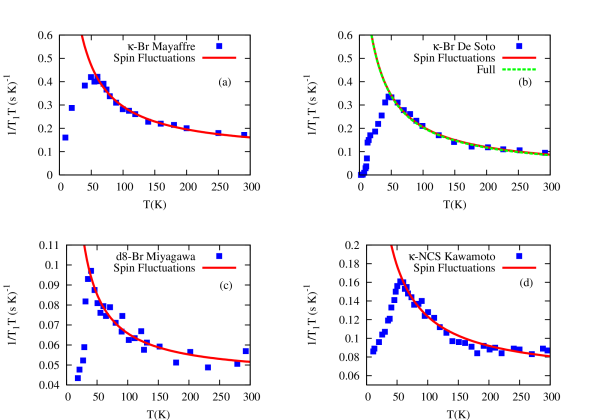
Figure 1: [Color online] Comparison of the measured nuclear spin relaxation rate per unit temperature, $1/T_{1}T$, with the predictions of the spin fluctuation model for various organic charge transfer salts. Panel (a) shows data for $\kappa$-(ET)₂Cu[N(CN)₂]Br measured by Mayaffre et al.mayaffre, panel (b) shows data for $\kappa$-(ET)₂Cu[N(CN)₂]Br measured by De Soto et al.desoto, panel (c) shows data for $\kappa$(d8)-(ET)₂Cu[N(CN)₂]Br measured by Miyagawa et al.miyagawa, and panel (d) shows data for a $\kappa$-(ET)₂Cu(NCS)₂ powder sample measured by Kawamoto et al.kawamoto The $1/T_{1}T$ data are weakly temperature dependent at high temperatures, have a maximum at $T_{\mathrm{NMR}}\sim 50$ K, and drop abruptly below $T_{\mathrm{NMR}}$, contrary to what one would expect for a Fermi liquid in which $1/T_{1}T$ is constant. The remarkable similarities of these data results from the quantitative and qualitative similarity of the antiferromagnetic spin fluctuations in the paramagnetic metallic phases of these materials. The parameters that produce the best fits (solid lines) to Eq. (13) are tabulated in Table 1. The spin fluctuation model gives a good fit to the experimental data between $T_{\mathrm{NMR}}\sim 50$ and room temperature which suggests strong spin fluctuations in the paramagnetic metallic states of $\kappa$-(ET)₂Cu[N(CN)₂]Br, $\kappa$(d8)-(ET)₂Cu[N(CN)₂]Br, and $\kappa$-(ET)₂Cu(NCS)₂. However, below $T_{\mathrm{NMR}}$ the spin fluctuation model does not describe the data well. In section V we argue that this is because a pseudogap opens at $T_{\mathrm{NMR}}$. In each figure the solid line indicates the large $T$ approximation of the spin fluctuation model [Eq. (15b)]. To check that this approximation is reasonable we also plot the full spin fluctuation model [Eq. (13)] as a dashed line in panel (b). The full and dashed lines cannot be distinguished until well below $T_{\mathrm{NMR}}$ and so we concluded that the high $T$ approximation is excellent in the relevant regime. Note that the analysis on $1/T_{1}T$ cannot differentiate between antiferromagnetic and ferromagnetic spin fluctuations (see section II.1.2), but the Korringa ratio strongly differentiates between these two case and indicates that the fluctuations are antiferromagnetic (see Fig. 2). The nomenclature $\kappa$-Br, d8-Br, and $\kappa$-NCS is used as shorthand for $\kappa$-(ET)₂Cu[N(CN)₂]Br, $\kappa$(d8)-(ET)₂Cu[N(CN)₂]Br, and $\kappa$-(ET)₂Cu(NCS)₂ respectively in the figure keys.

As well as their interesting phenomenology the organic charge transfer salts are important model systems and a deeper understanding of these materials may help address a number of important fundamental questions concerning strongly correlated systems. The (non-interacting) band structure of the $\kappa$ phase salts is well approximated by the half-filled tight binding model on the anisotropic lattice.powell:review This model has two parameters $t$, the hopping integral between nearest neighbor (ET)₂ dimers, and $t^{\prime}$, the hopping integral between next nearest neighbors across one diagonal only. In order to describe strongly correlated phases of these materials we must also include the effects of the Coulomb interaction between electrons. The simplest model which can include these strong correlations in the Hubbard model contains one additional parameter over the tight binding model: $U$, the Coulomb repulsion between two conduction electrons on the same dimer. In the Hubbard model picture the different $\kappa$-(ET)${}_{2}X$ salts and different pressures correspond to different values of $t^{\prime}/t$ and $U/t$, but all of the $\kappa$ phase salts are half filled. Varying $U/t$ allows us to tune the proximity to the Mott transition - understanding the Mott transition and its associated phenomena remains one most important problems in theoretical physicsgebhard; imada:rmp and the organics have provided a new window on this problem.kagawa; merino; limelette; powell:review; kanoda-thermo Varying $t^{\prime}/t$ allows one to tune the degree of frustration in the system. Understanding the effect of frustration in strongly correlated systems is of general importance.takada; Greedan; ong:frustration For example there are strong analogies between the organics and Na_xCoO₂,nacoo and much recent interest has been sparked by the observation of possible spin liquid states in organic charge transfer salts.shimizu; kato; kato2

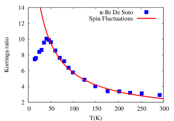
Figure 2: [Color online] Comparison of the Korringa ratio ${\cal K}\propto 1/T_{1}TK_{s}^{2}$ of $\kappa$-(ET)₂Cu[N(CN)₂]Br measured by De Soto et al.desoto with the prediction of the antiferromagnetic spin fluctuation model. The best fit to Eq. (III.2) is indicated by the solid line. The Korringa ratio is larger than 1 which indicates that the spin fluctuations are antiferromagnetic (${\cal K}<1$ for ferromagnetic fluctuations, see Section II.1.2). The antiferromagnetic correlation length is found to be $3.5\pm 2.5$ lattice spacings at 50 K. Below 50 K the Korringa ratio is suppressed, and in section V we argue that this is because a pseudogap opens at $T_{\mathrm{NMR}}$. In the key to this figure $\kappa$-(ET)₂Cu[N(CN)₂]Br is abbreviated as $\kappa$-Br.

The paramagnetic metallic phases of $\kappa$-(ET)${}_{2}X$ are very different from a conventional metallic phase. Many features of the paramagnetic metallic phases agree well with the predictions of dynamical mean field theory (DMFT) which describes crossover from ‘bad metal’ at high temperatures to a Fermi liquid as the temperature is lowered.merino; Jaime-HH-DMFT; hassan; limelette This crossover from incoherent to coherent intralayer transport has been observed in a number of experiments such as resistivity,limelette thermopower,yu; merino and ultrasonic attenuation.frikach; fournier The existence of coherent quasiparticles is also apparent from the observed magnetic quantum oscillations at low temperatures in $\kappa$-(ET)${}_{2}X$.singleton; wosnitza; kartsovnik However, nuclear magnetic resonance experiments (reproduced in Figs. 1 and 2) on the paramagnetic metallic phases on $\kappa$-(ET)${}_{2}X$ do not find the well known properties of a Fermi liquid. The nuclear spin relaxation rate per unit temperature, $1/T_{1}T$, is larger than the Korringa form predicted from Fermi liquid theory. As the temperature is lowered $1/T_{1}T$ reaches a maximum; we label this temperature $T_{\mathrm{NMR}}$ (the exact value of $T_{\mathrm{NMR}}$ varies with the anion $X$, but typically, $T_{\mathrm{NMR}}\sim 50$ K, see Fig. 6). $1/T_{1}T$ decreases rapidly as the temperature is lowered below $T_{\mathrm{NMR}}$ [see Fig 1].mayaffre; desoto; miyagawa:chemrev The Knight shift also drops rapidly around $T_{\mathrm{NMR}}$ [see Fig 4].desoto This is clearly in contrast the Korringa-like behavior one would expect for a Fermi liquid in which $1/T_{1}T$ and $K_{s}$ are constant for $T\ll T_{F}$, the Fermi temperature. Similar non-Fermi liquid temperature dependences of $1/T_{1}T$ and $K_{s}$ are observed in the cuprates.timusk; norman:adv For the cuprates, it has been argued that the large enhancement of $1/T_{1}T$ is associated with the growth of antiferromagnetic spin fluctuation within the CuO₂ planes as the temperature is lowered.moriya; millis The large decrease observed in $1/T_{1}T$ and $K_{s}$ is suggestive of a depletion of the density of states (DOS) at the Fermi level which might be expected if a pseudogap opens at $T_{\mathrm{NMR}}$.

A qualitative description of spin fluctuations in the paramagnetic metallic phase of $\kappa$-(ET)${}_{2}X$ has not been performed previously. The importance of spin fluctuations in $\kappa$-(ET)${}_{2}X$ below $T_{\mathrm{c}}$ has been pointed out by several groups.powell:review; schmalian; kino; jujo; ben:prl; kuroki Since the nature of the paramagnetic metallic and superconducting phases are intimately intertwined (in most theories, including BCS, superconductivity arises from an instability of the metallic phase), it is important to understand whether the spin fluctuations may extend beyond the superconducting region into the paramagnetic metallic phase and if so how strong they are. Another unresolved puzzle is whether there is a pseudogap in the paramagnetic metallic phase of $\kappa$-(ET)${}_{2}X$ which suppresses the density of states (DOS) at the Fermi level. A pseudogap has been suggested on the basis of the NMR data and heat capacity measurement.kanoda:jspj2006 If there is a pseudogap then important questions to answer include: (i) how similar is the pseudogap in $\kappa$-(ET)${}_{2}X$ to the pseudogaps in the cuprates, manganites and heavy fermions? (ii) is the pseudogap in $\kappa$-(ET)${}_{2}X$ related to superconductivity? and (iii) if so how?

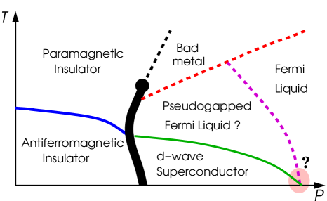
Figure 3: [Color online] The schematic phase diagram for $\kappa$-(ET)₂X as a function of temperature and pressure. Thin solid lines represent second order phase transitions, the thick solid line is the first order transition line which ends at a critical point shown as a filled circle, and dashed lines indicate crossovers. The pseudogap phase is much more complicated than a renormalized Fermi liquid that has been previously thought to characterize the paramagnetic metallic phase at low temperatures: it shows a coherent transport character with long lived quasiparticles, marked by $T^{2}$ resistivity behaviorlimelette and magnetic quantum oscillations,singleton but at the same time it exhibits a loss of density of states which is clearly seen in the NMR data. There are not sufficient data at this moment to determine where the pseudogap phase boundary ends so this uncertainty is represented by the shaded area with the question mark. More detailed experimental and theoretical studies in the vicinity of this point will give important insight into how the pseudogap is related to superconductivity. The possibility of a quantum critical point somewhere in the vicinity of the point where the superconducting critical temperature goes to zero may have important consequences for the observation that the materials with the lowest superconducting critical temperatures have extremely small superfluid stiffnesses and are very different from BCS superconductors.ujjual; pratt; constraints

A number of scenarios in which a pseudogap may arise have been proposed. One possible origin of a pseudogap, which a number of authorsben:prl; trivedi; zhang; ben:d+id; powell:review have argued may be relevant to the organic charge transfer salts, is the resonating valence bond (RVB) picture (for a review see Refs. lee and anderson). In this picture the electron spins form a linear superposition of spin singlet pairs. The singlet formation can naturally explain the appearance of a gap: a non-zero amount of energy is required to break the singlet pairs. For weakly frustrated lattices, such as the anisotropic triangular lattice in the parameter range appropriate for $\kappa$-(ET)₂Cu[N(CN)₂]Br, $\kappa$-(ET)₂Cu(NCS)₂, and $\kappa$-(ET)₂Cu[N(CN)₂]Cl, the RVB theory predicts ‘$d$-wave’ superconductivity.ben:prl; kuroki; trivedi; zhang; ben:d+id; powell:review This is the symmetry most consistent with a range of experiments on these $\kappa$-(ET)${}_{2}X$ salts.miyagawa:chemrev; powell:prb2004; analytis; powell:group However, as the frustration is increased changes in the nature of the spin fluctuations drive changes in the symmetry of the superconducting state.ben:d+id; powell:group For example, for the isotropic triangular lattice $t=t^{\prime}$ [$t\sim t^{\prime}$ is thought to be appropriate for $\kappa$-(ET)₂Cu₂(CN)₃] RVB theory predicts that the superconducting order parameter has ‘$d+id$’ symmetry.ben:d+id; powell:group

RVB theory also predicts that a pseudogap with the same symmetry as the superconducting state exists in the paramagnetic phase at temperatures above the superconducting critical temperature, $T_{c}$. This pseudogap results from the formation of short range singlets above $T_{c}$; only at $T_{c}$ do these singlets acquire off-diagonal long-range order. There are two energy scales ($\Delta$ and $\widetilde{\Delta}$ in the notation of, e.g., Refs. ben:prl and zhang) in the RVB theory. In the simplest reading of the theory,zhang-rmft; anderson the ratio $\Delta/\widetilde{\Delta}\approx T^{*}/T_{c}$ where $T^{*}$ is the temperature at which the pseudogap opens. For the appropriate model Hamiltonian for the layered $\kappa$-(ET)${}_{2}X$ salts $\Delta/\widetilde{\Delta}\simeq 5$ near the Mott transitionben:prl which is remarkably similar to the ratio $T_{\mathrm{NMR}}/T_{c}$ in $\kappa$-(ET)₂Cu[N(CN)₂]Br.

We use the phenomenological antiferromagnetic spin fluctuation model which was first introduced by Moriyamoriya and then applied by Millis, Monien and Pines (MMP)millis to cuprates, to examine the role of spin fluctuations in the paramagnetic metallic phase of $\kappa$-(ET)${}_{2}X$. We investigate whether the anomalous temperature dependences of NMR data can be explained without invoking a pseudogap in the DOS. We fit the spin fluctuation model to the nuclear spin relaxation rate per unit temperature $1/T_{1}T$, Knight shift $K_{s}$, and Korringa ratio $\mathcal{K}$ data and find that the large enhancements measured in $1/T_{1}T$ and $\mathcal{K}$ above $T_{\mathrm{NMR}}$ are the result of large antiferromagnetic spin fluctuations [see Figs. 1 and 2]. The correlation of the antiferromagnetic spin fluctuations increases as temperature decreases and the relevant correlation length is found to be $3.5\pm 2.5$ lattice spacings at $T=50$ K. The model produces reasonable agreement with experimental data down to $T\sim 50$ K. Below 50 K, $1/T_{1}T$ is suppressed but never saturates to a constant expected for a Fermi liquid while the spin fluctuation model produces a monotonically increasing $1/T_{1}T$ with decreasing temperature. We argue that this discrepancy between theory and experiment is due to the appearance of a pseudogap, not captured by the spin fluctuation model, which suppresses the DOS at the Fermi level.

Our results suggest the paramagnetic metallic phase of $\kappa$-(ET)${}_{2}X$ is richer than a renormalized Fermi liquid as has been previously thought to describe the low temperature metallic state. An exotic regime similar to the pseudogap in the cuprates appears to be realized in the paramagnetic metallic phase of $\kappa$-(ET)${}_{2}X$. Thus we believe the appropriate phase diagram of $\kappa$-(ET)${}_{2}X$ looks like the one sketched in Fig. 3. However, the pseudogap in $\kappa$-(ET)${}_{2}X$ is rather peculiar. On one hand, it shows a coherent intralayer transport (apparent from the $T^{2}$ resistivity and the observed quantum oscillations). On the other hand it also shows a loss of DOS apparent from $1/T_{1}T$ and $K_{s}$. Therefore it is important to emphasize that the pseudogap phase proposed for $\kappa$-(ET)${}_{2}X$ is different from the pseudogap phase realized in the cuprates. Understanding these differences may well provide important insight into the physics of the pseudogaps in both classes of material. We will discuss this matter further in Section V.

We have also applied the spin fluctuation formalism to the Mott insulating phase $\kappa$-(ET)₂Cu₂(CN)₃ (which may have a spin liquid ground state).shimizu While a reasonable agreement between the calculated and the experimental data on $1/T_{1}T$ has been obtained, the result for the Knight shift does not agree with the data. We believe that this discrepancy reflects the failure of the assumption that the peak in the dynamic susceptibility dominates even the long wavelength physics implicit in the spin-fluctuation model. The failure of this assumption is consistent with the strong frustration in $\kappa$-(ET)₂Cu₂(CN)₃ and the observed spin-liquid behavior of this material.shimizu; powell:review We show that there are qualitative as well as quantitative difference between the spin fluctuations in $\kappa$-(ET)₂Cu₂(CN)₃ and the spin fluctuations in the other $\kappa$-phase salts discussed in this paper.

The structure of the paper is as follows. In Section II we introduce the temperature dependence of the nuclear spin relaxation rate, spin echo decay rate, Knight shift, and Korringa ratio and describe how they probe spin fluctuations by probing the dynamical susceptibility. We calculate these properties in a number of approximations and contrast the results. In Section III we demonstrate that the spin fluctuation model provides reasonable fits to the existing experimental results for $\kappa$-(ET)${}_{2}X$ and discuss its limitations when applied to those materials. Section IV deals with the application of the spin fluctuation model to the spin liquid compound $\kappa$-(ET)₂Cu₂(CN)₃. We discuss the nature and extent of the pseudogap in Section V. Finally, in Section VI we suggest new experiments and give our conclusions.

II The Spin Lattice Relaxation Rate, Spin Echo Decay Rate, and Knight Shift

The temperature dependence of the nuclear spin lattice relaxation rate $1/T_{1}T$, spin echo decay rate $1/T_{2}$, Knight shift $K_{s}$, Korringa ratio ${\cal K}$, and the real and imaginary part of the dynamic susceptibility, $\chi^{\prime}({\bf q},\omega)$ and $\chi^{\prime\prime}({\bf q},\omega)$, defined by

$$\chi({\bf q},\omega)=\int d^{3}r~{}dte^{i({\bf q}\cdot{\bf r}-\omega t)}\chi({\bf r},t).$$ (1)

are discussed in this section. The general expressions for these quantities arebarzykin

$$\frac{1}{T_{1}} = \lim_{\omega\to 0}\frac{2k_{B}T}{\gamma_{e}^{2}\hbar^{4}}\sum_{\bf q}|A({\bf q})|^{2}\frac{\chi^{\prime\prime}({\bf q},\omega)}{\omega},$$ (2a)

$$\frac{1}{T^{2}_{2}} = \frac{2f_{A}}{\hbar^{6}\gamma_{e}^{4}}\sum_{\bf q}|A({\bf q})|^{4}\chi^{\prime}({\bf q},0)^{2},$$ (2b)

$$K_{s} = \frac{|A({\bf 0})|\chi^{\prime}({\bf 0},0)}{\gamma_{e}\gamma_{N}\hbar^{2}},$$ (2c)

and

$$\mathcal{K} = \frac{\hbar}{4\pi k_{B}}\left(\frac{\gamma_{e}}{\gamma_{N}}\right)^{2}\frac{1}{T_{1}TK_{s}^{2}},$$ (2d)

where $A({\bf q})$ is the hyperfine coupling between the nuclear and electron spins, $\gamma_{N}$ ($\gamma_{e}$) is the nuclear (electronic) gyromagnetic ratio, and $f_{A}$ is the relative abundance of the nuclear spin. For simplicity we will often consider a momentum independent hyperfine coupling $|A|$ in what follows. Note that Eqs. 2 show that this is an uncontrolled approximation for both $T_{1}$ and $T_{2}$, but that it is not an approximation at all for $K_{s}$. This is because $K_{s}$ only probes the long wavelength physics and hence only depends on $A({\bf 0})$, the hyperfine coupling at ${\bf q}=\bf 0$.

The calculation of the quantities in Eqs. (2) boils down to determining the appropriate form of the dynamic susceptibility. In the following sections we begin by discussing the role of vertex corrections in determining the properties measured by NMR (section LABEL:sect:vertex), before moving onto the a variety of approximations for calculating the dynamic susceptibility. They are antiferromagnetic and ferromagnetic spin fluctuations (section II.1), dynamical mean field theory (section II.2), and the $1/N$ approach to the quantum critical region of frustrated two-dimensional antiferromagnets (section II.3). However, in this work we will predominantly use the spin fluctuation model to analyze the NMR data. The other models are presented for comparison.

II.1 The Spin Fluctuation Model

The dynamic susceptibility in this model is written asmoriya; millis

$$\chi({\bf q},\omega)=\chi_{\mathrm{LW}}(\omega)+\chi_{\mathrm{AF}}({\bf q},\omega),$$ (3)

where $\chi_{\mathrm{LW}}(\omega)$ is the dynamic susceptibility in the long wavelength regime and $\chi_{\mathrm{AF}}({\bf q},\omega)$ is a contribution to the dynamic susceptibility which peaks at some wave vector ${\bf Q}$. These susceptibilities take the form

$$\chi_{\mathrm{LW}}(\omega) = \frac{\bar{\chi}_{0}(T)}{1-i\omega/\Gamma(T)}$$

$$\chi_{\mathrm{AF}}({\bf q},\omega) = \frac{\chi_{Q}(T)}{1+\xi(T)^{2}|{\bf q}-{\bf Q}|^{2}-i\omega/\omega_{\mathrm{SF}}(T)}$$ (4)

where $\bar{\chi}_{0}(T)$ [$\chi_{Q}(T)$] is the static spin susceptibility at ${\bf q}={\bf 0}$ [${\bf Q}$], $\Gamma(T)$ [$\omega_{\mathrm{SF}}(T)$] is the characteristic spin fluctuation energy which represents damping in the system near ${\bf q}={\bf 0}$ [${\bf Q}$], and $\xi(T)$ is the temperature dependent correlation length. Hence, the real and imaginary parts of the dynamic susceptibility can then be written as

$$\chi^{\prime}({\bf q},0) = \bar{\chi}_{0}(T)\left[1+\frac{\chi_{Q}(T)}{\bar{\chi}_{0}(T)}\frac{1}{(1+\xi(T)^{2}|{\bf q}-{\bf Q}|^{2})^{2}}\right]$$

$$\chi^{\prime\prime}({\bf q},\omega) = \frac{\omega\bar{\chi}_{0}(T)}{\Gamma}$$

$$\left[1+\frac{\chi_{Q}(T)\Gamma}{\bar{\chi}_{0}(T)\omega_{\mathrm{SF}}(T)}\frac{1}{(1+\xi(T)^{2}|{\bf q}-{\bf Q}|^{2})^{2}}\right].$$

Note that the above form of $\chi_{LW}(\omega)$ is the appropriate form for a Fermi liquid. Therefore if the system under discussion is not a Fermi liquid then the validity this expression for $\chi_{LW}(\omega)$ cannot be guaranteed. For example, the marginal Fermi liquid theory predicts a different frequency dependence.varma If the dynamic susceptibility is sufficiently peaked then $1/T_{1}$ will not be strongly dependent on the long wavelength physics [because $1/T_{1}$ measures the susceptibility over the entire Brillouin zone, c.f., Eq. (2a), and therefore will be dominated by the physics at ${\bf q}=\bf Q$]. On the other hand the Knight shift is a measure of the long wavelength properties [c.f., Eq. (2c)] and therefore may be sensitive to the details of $\chi_{\mathrm{LW}}(\omega)$. Here we will explicitly assume, following the assumption made by MMPmillis, that the uniform susceptibility $\bar{\chi_{0}}$ and the spin fluctuation energy near $q=0$ is temperature independent. One justification for this approximation in organics is that the Knight shift is not strongly temperature dependent [see Section III D]. This approximation will break down in the systems where the uniform susceptibility is strongly temperature dependent such as YBa₂Cu₃O_6.63monien:prb43 and La_1.8Sr_0.15CuO₄.monien:prb43b

In the critical region $\xi(T)\gg a$, where $\xi(T)$ is the correlation length, and $a$ is the lattice constant, and one hasmillis

$$\chi_{Q}(T) = \left(\frac{\xi(T)}{\xi_{0}}\right)^{2-\eta}\bar{\chi_{0}}$$

$$\omega_{\mathrm{SF}}(T) = \left(\frac{\xi_{0}}{\xi(T)}\right)^{z}\Gamma$$ (6)

where $\eta$ is the critical exponent which governs the power-law decay of the spin correlation function, $z$ is the dynamical critical exponent, and $\xi_{0}$ is some temperature independent length scale. The simplest possible assumptions are relaxation dynamics for the spin fluctuations (which are characterized by $z=2$) and mean field scaling of the spin correlations ($\eta=0$). With these approximations the real and imaginary parts of the dynamic susceptibility are given by

$$\chi^{\prime}({\bf q},0) = \bar{\chi}_{0}\left[1+\sqrt{\beta}\frac{[\xi(T)/a]^{2}}{[1+\xi(T)^{2}|{\bf q}-{\bf Q}|^{2}]^{2}}\right]$$

$$\chi^{\prime\prime}({\bf q},\omega) = \frac{\omega\bar{\chi}_{0}}{\Gamma}\left[1+\beta\frac{[\xi(T)/a]^{4}}{[1+\xi(T)^{2}|{\bf q}-{\bf Q}|^{2}]^{2}}\right]$$ (7)

where $\beta=(a/\xi_{0})^{4}$. The temperature independent, dimensionless parameter $\beta$ can also be expressed in terms of the original variables appearing in the dynamic susceptibility in Eq. (4) as

$$\beta=\frac{\chi_{Q}(T)\Gamma}{\bar{\chi}_{0}\omega_{\mathrm{SF}}(T)}\left(\frac{a}{\xi(T)}\right)^{4}.$$ (8)

Written in this form, $\beta$ has a clear interpretation: it represents the strength of the spin fluctuations at a finite wave vector $\bf Q$. We will now consider two cases: antiferromagnetic and ferromagnetic spin fluctuations.

II.1.1 Antiferromagnetic Spin Fluctuations

If we have antiferromagnetic spin fluctuations then the dynamic susceptibility $\chi({\bf q},\omega)$ peaks at a finite wave vector ${\bf q}={\bf Q}$; for example, for a square lattice ${\bf Q}=(\pi,\pi)$. The NMR relaxation rate, spin echo decay rate, and Knight shift can be calculated straightforwardly from the real and imaginary parts of the dynamic susceptibility given in Eq. (LABEL:real_im_af). The results are

$$\frac{1}{T_{1}T} = \frac{2\pi k_{B}|A|^{2}\bar{\chi}_{0}}{\gamma_{e}^{2}\hbar^{4}\Gamma}\left[1+\beta\frac{[\xi(T)/a]^{4}}{1+[\tilde{Q}\xi(T)]^{2}}\right]$$ (9a)

$$\frac{1}{T_{2}^{2}} = \frac{2f_{A}|A|^{4}\bar{\chi}_{0}^{2}}{\pi\gamma_{e}^{4}\hbar^{6}}\bigg{[}1+\beta\frac{[\xi(T)/a]^{4}}{1+[\tilde{Q}\xi(T)]^{2}}$$ (9b)

$$+\frac{\sqrt{\beta}}{\pi}\ln(1+[\tilde{Q}\xi(T)]^{2})\bigg{]}$$

$$K_{s} = \frac{|A|\bar{\chi}_{0}}{\gamma_{e}\gamma_{N}\hbar^{2}}\left[1+\sqrt{\beta}\frac{[\xi(T)/a]^{2}}{1+[\tilde{Q}\xi(T)]^{2}}\right]$$ (9c)

$${\cal K} = \frac{\hbar\gamma_{e}^{2}}{2\Gamma\bar{\chi}_{0}}\frac{\left[1+\beta\frac{[\xi(T)/a]^{4}}{1+[\tilde{Q}\xi(T)]^{2}}\right]}{\left[1+\sqrt{\beta}\frac{[\xi(T)/a]^{2}}{1+[\tilde{Q}\xi(T)]^{2}}\right]^{2}},$$ (9d)

where $\tilde{Q}$ is a cutoff from the momentum integration [c.f. Eq. (2a)]. For $\xi(T)\gg a$: $1/T_{1}T\sim\xi(T)^{2}$, $1/T_{2}\sim\xi(T)$, and $K_{s}\sim$ constant which leads to the Korringa ratio $\mathcal{K}\simeq(\hbar\gamma_{e}^{2}/2\Gamma\bar{\chi}_{0})[\tilde{Q}\xi(T)]^{2}$. In this model the Korringa ratio can only be equal to unity if the spin fluctuations are completely suppressed ($\beta=0$). Hence, one expects ${\cal K}>1$ if antiferromagnetic fluctuations are dominant.moriya:jpsj; narath This indicates that there are significant vertex corrections when there large strong antiferromagnetic fluctuations.

II.1.2 Ferromagnetic Spin Fluctuations

For ferromagnetic spin fluctuations, $\chi({\bf q},\omega)$ is peaked at ${\bf q}=\bf 0$. The NMR relaxation rate and spin echo decay rate are exactly the same as those given in Eqs. (9a) and (9b) because $1/T_{1}T$ and $1/T_{2}$ come from summing the contributions form all wave vectors in the first Brillouin zone, which makes the location of the peak in q space irrelevant. In contrast, the Knight shift will be different in the ferromagnetic and antiferromagnetic cases because $K_{s}$ only measures the ${\bf q}=\bf 0$ part of the dynamic susceptibility; it will be enhanced by the ferromagnetic fluctuations. Thus, in the ferromagnetic spin fluctuation description $K_{s}$ is given by

$$K_{s} = \frac{|A|\bar{\chi}_{0}}{\gamma_{e}\gamma_{N}\hbar^{2}}\left[1+\sqrt{\beta}(\xi/a)^{2}\right]$$ (10)

and

$${\cal K} = \frac{\hbar\gamma_{e}^{2}}{2\Gamma\bar{\chi}_{0}}\frac{\left[1+\beta\frac{[\xi(T)/a]^{4}}{1+[\tilde{Q}\xi(T)]^{2}}\right]}{\left[1+\sqrt{\beta}(\xi/a)^{2}\right]^{2}}$$ (11)

For $\xi(T)\gg a$: $1/T_{1}T\sim\xi(T)^{2}$, $1/T_{2}\sim\xi(T)$, and $K_{s}\sim\xi(T)^{2}$ which leads to $\mathcal{K}\simeq(\hbar\gamma_{e}^{2}/2\Gamma\bar{\chi}_{0})[\pi\xi(T)/a]^{-2}$. We can see that $\mathcal{K}<1$ in the presence of ferromagnetic fluctuations.moriya:jpsj; narath So again vertex corrections are important if the system has strong ferromagnetic fluctuations. Recall that, in contrast, in the case of antiferromagnetic fluctuations the Korringa ratio is larger than one. Thus analyzing the Korringa ratio allows one to straightforwardly distinguish between antiferromagnetic and ferromagnetic spin fluctuations.

II.2 Dynamical Mean Field Theory

DMFT is an approach based on a mapping of the Hubbard model onto a self-consistently embedded Anderson impurity model.georges; kotliar; pruschke DMFT predicts that the metallic phase of the Hubbard model has two regimes with a crossover from one to the other at a temperature $T_{0}$. For $T\textless T_{0}$ the system is a renormalized Fermi liquid characterized by Korringa-like temperature dependence of $1/T_{1}T$ and coherent intralayer transport. Above $T_{0}$, the system exhibits anomalous properties with $1/T_{1}T\sim a+b(T_{0}/T)$ (c.f., Ref. [pruschke]) and incoherent charge transport. This regime is often refereed to as the ‘bad metal’. Microscopically the bad metal is characterized by quasi-localized electrons and the absence of quasiparticles. Thus DMFT predicts that at high temperatures $1/T_{1}T\sim a+b(T_{0}/T)$, but $1/T_{1}T$ saturates to a constant below $T_{0}$. This temperature dependence is similar to that for the single impurity Anderson model.jarrell Note that this temperature dependence is qualitatively similar to that found for spin fluctuations [c.f., Eq. (15b), the high temperature limit of Eq. (9a)].

The predictions of DMFT correctly describe the properties of a range of transport and thermodynamic experiments on the organic charge transfer salts.merino; limelette; powell:review This suggests that these systems undergo a crossover from a bad metal regime for $T\textgreater T_{0}$ to a renormalized Fermi liquid below $T_{0}$. As we shall see in more detail later (see Fig. 1) the nuclear spin relaxation rate is suppressed but never saturates below $T_{\mathrm{NMR}}$; this is not captured by DMFT. This suggests that the low-temperature regime of $\kappa$-(ET)${}_{2}X$ is more complicated than the renormalized Fermi liquid predicted by DMFT which until now, is widely believed to be the correct description of the low temperature paramagnetic metallic state in the organic charge transfer salts. We will discuss the reasons for and implications of the failure of DMFT to correctly describe NMR experiments on the organic charge salts in section V.

II.3 Quantum Critical Region of Frustrated 2D Antiferromagnets

The static uniform and dynamic susceptibilities of nearly-critical frustrated 2D antiferromagnets has been studied by Chubukov et al.chubukov They considered a long-wavelength action with an $N$ component, unit-length, complex vector which has a SU($N$)$\otimes$O(2) symmetry and performed a $1/N$ expansion. This gives susceptibilities which follow a universal scaling form. As one approaches the quantum critical point, the spin stiffness will vanish but the ratio between in-plane and out-of-plane stiffnesses remains finite and approaches unity. In this regime, to order $1/N$, the quantities in Eq. (2) are given bychubukov

$$1/T_{1}\sim T^{\eta};~{}~{}1/T_{2}\sim T^{\eta-1};~{}~{}K_{s}\sim T;~{}~{}\mathcal{K}\sim T^{\eta-2}.$$ (12)

III Spin Fluctuations in $\kappa$-(ET)${}_{2}X$

The NMR relaxation rate per unit temperature, Knight shift, and Korringa ratio in the antiferromagnetic spin fluctuations model are given by Eqs. (9a), (9c), and (9d). Their temperature dependence comes through the antiferromagnetic correlation length. We adopt the form of $\xi(T)$ from M-MMPmoriya; millis: $\xi(T)/\xi(T_{x})=\sqrt{2T_{x}/(T+T_{x})}$. For this form of the correlation length $T_{x}$ represents a natural temperature scale and $\xi(T)$ is only weakly temperature dependent for $T\ll T_{x}$. For this choice of $\xi(T)/a$ we have

$$\frac{1}{T_{1}T} = \left(\frac{1}{T_{1}T}\right)_{0}\left[1+\frac{\beta C^{2}}{(T/T_{x}+1)^{2}+2\pi^{2}C(T/T_{x}+1)}\right]$$

$$K_{s} = (K_{s})_{0}\left[1+\frac{\sqrt{\beta}C}{1+2\pi^{2}C+T/T_{x}}\right]$$

$${\cal K} = {\cal K}_{0}\frac{\left[1+\frac{\beta C^{2}}{(T/T_{x}+1)^{2}+2\pi^{2}C(T/T_{x}+1)}\right]}{\left[1+\frac{\sqrt{\beta}C}{1+2\pi^{2}C+T/T_{x}}\right]^{2}},$$ (13)

where we have defined

$$C = 2\left[\frac{\xi(T_{x})}{a}\right]^{2},$$

$$(1/T_{1}T)_{0} = \frac{2\pi k_{B}|A|^{2}\bar{\chi}_{0}}{\gamma_{e}^{2}\hbar^{4}\Gamma},$$

$$(K_{s})_{0} = \frac{|A|\bar{\chi}_{0}}{\gamma_{e}\gamma_{N}\hbar^{2}},$$

$$\textrm{and}~{}~{}{\cal K}_{0} = \frac{\hbar\gamma_{e}^{2}}{2\Gamma\bar{\chi}_{0}},$$ (14)

to simplify the notation.

III.1 The Nuclear Spin Relaxation Rate

We now analyze the temperature dependence of $1/T_{1}$. In the discussion to follow, we will assume that the correlation length is large compared to unity and to $T/T_{x}$, i.e, $C=2(\xi(T_{x})/a)^{2}\gg T/T_{x}$. By this assumption, the limiting cases of $1/T_{1}T$ [Eq. (13)] are given by

$$\frac{(T_{1}T)_{0}}{T_{1}T} \simeq 1+\frac{\beta}{\pi^{2}}\left(\frac{\xi(T_{x})}{a}\right)^{2}\left[1-\left(\frac{T}{T_{x}}\right)\right]$$ (15a)

$$\mathrm{for}~{}T\ll T_{x}$$

$$\frac{(T_{1}T)_{0}}{T_{1}T} \simeq 1+\frac{\beta}{\pi^{2}}\left(\frac{\xi(T_{x})}{a}\right)^{2}\left(\frac{1}{T/T_{x}+1}\right)$$ (15b)

$$\mathrm{for}~{}T\gg T_{x}.$$

The NMR relaxation rate per unit temperature calculated from the spin fluctuation model is a monotonic function of temperature. In the high-temperature regime $1/T_{1}T$ has a $T^{-1}$ dependence while in the low-temperature regime it is linear in $T$ with a negative slope. Thus one realizes immediately that the data for temperatures below $T_{\mathrm{NMR}}$ is not consistent with the predictions of the spin fluctuation theory as it has a positive slope. We will return to discuss this regime latter. We begin by investigating the high temperature regime, $T>T_{\mathrm{NMR}}$.

We fit the $1/T_{1}T$ expression for $T\gg T_{x}$ (15b) to the experimental data of De Sotodesoto for $\kappa$-(ET)₂Cu[N(CN)₂]Br  between $T_{\mathrm{NMR}}$ and 300 K with $(1/T_{1}T)_{0}$, $\beta[\xi(T_{x})/a]^{2}$, and $T_{x}$ as free parameters. It is not possible to obtain $\beta$ and $\xi(T_{x})/a$ unambiguously from fitting to $1/T_{1}T$ data because the model depends sensitively only on the product $\beta[\xi(T_{x})/a]^{2}$ (see Eq. (15b)). The parameters from the fits are tabulated in Table 1 and the results are plotted in Fig. 1. The use of Eq. (15b) to fit $1/T_{1}T$ data is justified post hoc since $T_{x}$ is found to be $2-6$ times smaller than $T_{\mathrm{NMR}}$. We have also checked this by plotting the full theory (without taking the $T\gg T_{x}$ limit) for $\kappa$-(ET)₂Cu[N(CN)₂]Br in Fig. 1b, where there is Korringa ratio data (see Fig. 2) and thus we can determine $\beta$ and $\xi(T_{x})/a$ individually. It can be seen from Fig. 1b that the disagreement between the full theory and the high temperature approximation is smaller than the thickness of the curves, therefore this approximation is well justified. It will be shown in Section II B that the correlation length is indeed large thus providing further justification for the use of Eq. (15b) here.

The model produces a reasonably good fit to the experimental data on $\kappa$-(ET)₂Cu[N(CN)₂]Brdesoto between $T_{\mathrm{NMR}}$, the temperature at which $1/T_{1}T$ is maximum, and room temperature. In the high temperature regime (e.g., around room temperature), $1/T_{1}T$ has a very weak temperature dependence, indicating weakly correlated spins. The large enhancement of $1/T_{1}T$ can be understood in terms of the growth of the spin fluctuations: as the system cools down, the spin-spin correlations grow stronger which allows the nuclear spins to relax faster by transferring energy to the rest of the spin degrees of freedom via these spin fluctuations. Strong spin fluctuations, measured by large values of $\beta[\xi(T_{x})/a]^{2}$, are not only present in $\kappa$-(ET)₂Cu[N(CN)₂]Br but also observed in other materials such as the fully deuterated $\kappa$-(ET)₂Cu[N(CN)₂]Br {which will be denoted by $\kappa$(d8)-(ET)₂Cu[N(CN)₂]Br} and $\kappa$-(ET)₂Cu(NCS)₂. The results of the fits for $\kappa$(d8)-(ET)₂Cu[N(CN)₂]Br and $\kappa$-(ET)₂Cu(NCS)₂ are shown in Fig. 1. The parameters that produce the best fits are also tabulated in Table 1. This suggests that strong spin fluctuations are present in these charge transfer salts. In all cases studied here, strong spin fluctuations are evident from the large value of $\beta[\xi(T_{x})/a]^{2}$.

The nature of the spin fluctuations, i.e., whether they are antiferromagnetic or ferromagnetic, cannot, even in principle, be determined from the analysis on $1/T_{1}T$. Both cases yield the same $1/T_{1}T$ [see Eq. (9) and Sec II.C.2] because the nuclear spin relaxation rate is obtained by summing all wave vector contribution in the first Brillouin zone. However, in the next section we will use the Korringa ratio to show that the spin fluctuations are antiferromagnetic.

Material	Ref.	$(1/T_{1}T)_{0}$	$T_{x}$ (K)	$\beta[\xi(T_{x})/a]^{2}$
		($s^{-1}$K-1)
$\kappa$-Br	Mayaffre [mayaffre]	0.09 $\pm$ 0.01	6.5 $\pm 5.5$	290 $\pm 250$
$\kappa$-Br	De Soto [desoto]	0.02 $\pm$ 0.01	20 $\pm 10$	680 $\pm 430$
d8-Br	Miyagawa [miyagawa]	0.04 $\pm 0.01$	6.2 $\pm 3.5$	85 $\pm 65$
$\kappa$-NCS	Kawamoto [kawamoto]	0.06 $\pm 0.01$	11 $\pm 2.6$	110 $\pm 89$

Table 1: The parameters obtained from the fits which are used to produce Fig. 1. Evidence for strong spin fluctuations come from the large value of $\beta[\xi(T_{x})/a]^{2}$ which are present for all the materials tabulated above. In the table $\kappa$-Br, d8-Br, and $\kappa$-NCS are used as shorthand for $\kappa$-(ET)₂Cu[N(CN)₂]Br, $\kappa$(d8)-(ET)₂Cu[N(CN)₂]Br, and $\kappa$-(ET)₂Cu(NCS)₂ respectively.

Below $T_{\mathrm{NMR}}$, the calculated $1/T_{1}T$ continues to rise while the experimental data shows a decrease in the nuclear spin relaxation rate per unit temperature. However, the data does not reach a constant $1/T_{1}T$ as expected for a Fermi liquid. This indicates that the physics below $T_{\mathrm{NMR}}$ is dominated by some other mechanism not captured by the spin fluctuation, Fermi liquid, or DMFT theories. One possibility is a pseudogap opens up at $T_{\mathrm{NMR}}$ which suppresses the DOS at the Fermi level. Since $1/T_{1}T\sim\tilde{\rho}^{2}(E_{F})$ [c.f., Eq. (40)], a decrease in DOS will naturally lead to the suppression of $1/T_{1}T$. One might argue that the discrepancy between the theory and experiments below $T_{\mathrm{NMR}}$ stems from our assumption of a q-independent hyperfine coupling in the $1/T_{1}T$ expression. However, in section III.4 we will show that the Knight shift is also inconsistent with the predictions of the spin fluctuation model below $T_{\mathrm{NMR}}$. While including the appropriate q-dependence of the hyperfine coupling might change the temperature dependence of $1/T_{1}T$, it certainly cannot affect the temperature dependence of the Knight shift as can be seen from Eq. (2c).

III.2 The Korringa Ratio

In the previous section we compared the prediction of the spin fluctuation model for $1/T_{1}T$ to the experimental data and obtained good agreement with the data between $T_{\mathrm{NMR}}$ and 300 K. However, we were not able to determine $\beta$ and $\xi(T_{x})/a$ unambiguously because $1/T_{1}T$ is sensitive only to the product $\beta[\xi(T_{x})/a]^{2}$. We were also not able to determine whether antiferromagnetic or ferromagnetic spin fluctuations are dominant. We resolve these by studying the Korringa ratio ${\cal K}$. It has previously been pointed out that antiferromagnetic (ferromagnetic) fluctuations produce a Korringa ratio that is larger (less) than one.moriya:jpsj; narath We have also shown in Section II that in the limit of large correlation length, the Korringa ratio behaves like $(\xi/a)^{2}>1$ for antiferromagnetic spin fluctuations and like $(a/\xi)^{2}<1$ for ferromagnetic spin fluctuations. The Korringa ratio data for $\kappa$-(ET)₂Cu[N(CN)₂]Br (see Fig 2) is significantly larger than one at all temperatures which shows that antiferromagnetic fluctuations dominate. With this in mind, we study the antiferromagnetic spin fluctuation model.

First we note that $K_{s}$, given by Eq. (13), has a weak temperature dependence because $C=2(\xi(T_{x})/a)^{2}$ is generally larger than unity and $T/T_{x}$. In the limit of large correlation lengths, the second term inside the square bracket in the expression for $K_{s}$ given in Eq. (13) can be approximated as $(1+C+T/T_{x})^{-1}\simeq C^{-1}$ and the Knight shift will be given by $K_{s}\simeq(K_{s})_{0}(1+\sqrt{\beta}/(2\pi^{2}))$ which is temperature independent. We use this temperature independent Knight shift to calculate the Korringa ratio $\cal{K}$

$${\cal K} = \frac{\hbar}{4\pi k_{B}}\left(\frac{\gamma_{e}}{\gamma_{N}}\right)^{2}\frac{1}{T_{1}TK_{s}^{2}}$$

$$\simeq {\cal K}_{0}\left(1+\frac{\beta[\xi(T_{x})/a]^{2}}{\pi^{2}(T/T_{x}+1)}\right)\left(\frac{1}{1+\sqrt{\beta}/(2\pi^{2})}\right)^{2}$$

where the prefactor ${\cal K}_{0}$ is given by Eq. (14).

We fit Eq. (III.2) to the experimental Korringa data for $\kappa$-(ET)₂Cu[N(CN)₂]Br.desoto The result is plotted in Fig. 2. In this expression we have three parameters, $\beta[\xi(T_{x})/a]^{2}$, $T_{x}$, and $\sqrt{\beta}$, two of which, $\beta[\xi(T_{x})/a]^{2}$ and $T_{x}$, have been determined from fitting $1/T_{1}T$. There is only one remaining free parameter in the model, $\sqrt{\beta}$, which can then be determined unambiguously from the Korringa fit which yields $\beta=60\pm 20$. This value of $\beta$ implies that the antiferromagnetic correlation length $\xi(T)=3.5\pm 2.5a$ ($a$ is the unit of one lattice constant) at $T=50$ K. This value is in the same order of magnitude as the value of the correlation length estimated in the cuprates.monien:prb43

The Korringa ratio data are well reproduced by the antiferromagnetic spin fluctuation model when $T>T_{\mathrm{NMR}}$. This is again consistent with our earlier conclusion that the spin fluctuations have antiferromagnetic correlations. A large Korringa ratiotakigawa:physica_c; bulut has previously been observed in the cuprates indicating similar antiferromagnetic fluctuations in these systems. The Korringa ratio has also been measured in a number of heavy fermion compoundsishida; aart; kitaoka Similar antiferromagnetic fluctuations, like those observed in the cuprates and organics, are present in CeCu₂Si₂ and. The Korringa ratio of this material has a value of 4.6 at 100 mK (Ref. [aart]). In contrast, YbRh₂Si₂ishida and CeRu₂Si₂kitaoka, show strong ferromagnetic spin fluctuations as is evident from the Korringa ratio less than unity. In Sr₂RuO₄ishida:ruthenates the Korringa ratio is approximately 1.5 at 1.4 K. Upon doping with Ca to form Sr_2-xCa_x2RuO₄, the Korringa ratio becomes less than one which indicates that there is a subtle competition between antiferromagnetic and ferromagnetic fluctuations in these ruthenates.

III.3 The Antiferromagnetic Correlation Length

It is important to realize that the spin fluctuation formalism can be used to extract quantitative information about the spin correlations from NMR data. For example, the fits presented in Figs. 1 and 2 allow us to estimate the antiferromagnetic correlation length. From the fit for $\kappa$-(ET)₂Cu[N(CN)₂]Br (Table 1) we found that the antiferromagnetic correlation length $\xi(T)/a=3.5\pm 2.5$ at $T=T_{\mathrm{NMR}}=50$ K. In order to understand the physical significance of this value of $\xi(T)$ it is informative to compare this value with the correlation length for the squareding and triangularelstner lattice antiferromagnetic Heisenberg models.

It has been shownding that, on the square lattice, the antiferromagnetic Heisenberg model has a correlation length of order $\xi(T)/a\sim 1$ for $T=J$ and of order $\xi(T)/a\sim 30$ for $T=0.3J$. On the other hand for the antiferromagnetic Heisenberg model on the isotropic triangular lattice, the correlation length is only of order a lattice constant at $T=0.3J$.elstner Thus the correlation length, $\xi(T)/a=3.5\pm 2.5$, obtained from the analysis of the data for $\kappa$-(ET)₂Cu[N(CN)₂]Br is reasonable and places the materials between the square and isotropic antiferromagnetic Heisenberg model as has been argued on the basis of electronic structure calculations.mckenzie:comments; kino; powell:review

One of the best ways to measure antiferromagnetic correlation length is by inelastic neutron scattering experiments. To perform this experiment, one needs high quality single crystal. Unfortunately, it is difficult to grow sufficiently large single crystals for $\kappa$-(ET)${}_{2}X$; however, recently some significant progress has been made.taniguchi-cry Another way to probe the correlation length is through the spin echo experiment. The spin echo decay rate $1/T_{2}$ is proportional to the temperature dependence correlation length [see Eq. (9)] so measurements of $T_{2}$ would give us direct knowledge on the nature of the correlation length. To the authors’ knowledge there is no spin echo decay rate measurement on the metallic phase of the layered organic materials at the present time thus it is very desirable to have experimental data on $T_{2}$ measurement to compare with the value of $\xi(T)$ we have extracted above.

III.4 The Knight Shift

As we pointed out in Section II the Knight shift $K_{s}$ will generally have a weak temperature dependence throughout the whole temperature range and so, thus far, we have neglected its temperature dependence. However, it is apparent from Eq. (13) that for any choice of parameter values $\{\beta,\xi(T_{x})/a$, and $T_{x}\}$, $K_{s}$ will always increase monotically as the temperature decreases. Therefore the temperature dependence of the Knight shift potentially provides an important check on the validity of the spin fluctuation model. However, in the following discussion one should recall the caveats (discussed in section II.1) on the validity of the calculation of the Knight shift stemming from the assumption that the dynamics of the long wavelength part of dynamical susceptibility relax in the same manner as a Fermi liquid.

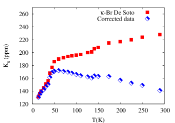
Figure 4: The temperature dependence of the (constant pressure) Knight shift as measured by $\kappa$-(ET)₂Cu[N(CN)₂]Br by De Soto et al.desoto (filled squares) and the corrected Knight shift obtained by taking into account thermal expansion of the lattice (half-filled diamonds), i.e., the constant volume Knight shift. The temperature at which the Knight shift decreases rapidly is about the same temperature at which $1/T_{1}T$ is suppressed (see Fig. 1), i.e. $T_{K_{s}}\sim T_{\mathrm{NMR}}$. This suggests that $1/T_{1}T$ and $K_{s}$ are suppressed by the same physics. In the limit of large correlation lengths, the spin fluctuation model, Eq. (13), predicts a slowly varying Knight shift which is almost temperature independent (solid line). The discrepancy between theory and experiment arises because the model calculates constant volume Knight shift while the experiment measures constant pressure Knight shift.wzietek Since $\kappa$-(ET)${}_{2}X$ is soft there will be a sizeable effect on $K_{s}$ due to the large thermal expansion. The correction to the experimental Knight shift, by taking into account these effects, was calculated by using Eq. (III.4) (half filled squares). However, we stress that the lack of compressive measurements of pressure and temperature dependence of the Knight shift, isothermal compressibility, and thermal expansion means that this correction is no better than an order of magnitude estimate. However, our estimate indicates that there correction is large enough that the data above $T_{K_{s}}$ cannot be shown to be in disagreement with the spin fluctuation model. Below $T_{K_{s}}$ there is a clear disagreement between the theory and data, in section V we argue that this is because a pseudogap opens at $T_{\mathrm{NMR}}$. In the key to this figure $\kappa$-(ET)₂Cu[N(CN)₂]Br is abbreviated as $\kappa$-Br.

In contrast to the prediction of the spin fluctuation model the experimental data, e.g., those measureddesoto on $\kappa$-(ET)₂Cu[N(CN)₂]Br (reproduced in Fig. 4), show that $K_{s}$ decreases slowly with decreasing temperature which then undergoes a large suppression around $T_{K_{s}}\sim 50$ K. It should be emphasized here that $T_{K_{s}}$ is approximately the same as $T_{\mathrm{NMR}}$, the temperature at which $1/T_{1}T$ is maximum.

Since it is not possible to explain any of the NMR data below $T_{\mathrm{NMR}}$ in terms of the spin fluctuation model within the approximations discussed thus far we focus on the temperature range between 50 K to 300 K just as we did for the analysis of $1/T_{1}T$. Even in this temperature range, there is a puzzling discrepancy between theory and experiment: the experimental data decreases slowly with decreasing temperature while the theoretical calculation predicts the opposite. We will argue below that this discrepancy arises because the data are obtained at constant pressure while the theoretical prediction assumes constant volume. Since the organic charge transfer salts are particularly soft, thermal expansion of the unit cell may produce a sizeable effect to the Knight shift and may not be neglected.

Following Wzietek et al.,wzietek we attempt to make an estimate on the correction of the Knight shift for $\kappa$-(ET)₂Cu[N(CN)₂]Br due to thermal expansion. Let us define $\chi_{s}^{v}(T,V)$ as the constant volume spin susceptibility as a function of temperature. The measured susceptibility is then given by a constant pressure susceptibility $\chi_{s}^{p}=\chi_{s}^{p}[T,V(T,P)]$ while the theoretical susceptibility is given by a constant volume susceptibility $\chi_{s}^{v}=\chi_{s}^{v}[T,V(T=0,P)]$. The correction to the spin susceptibility is then given by

$$\Delta\chi = \chi_{s}^{p}-\chi_{s}^{v}$$

$$= \int_{0}^{T}{dT^{\prime}}\left(\frac{\partial\chi_{s}^{p}}{\partial P}\right)_{T^{\prime}}\left(\frac{V\partial P}{\partial V}\right)_{T^{\prime}}\left(\frac{\partial V}{V\partial T^{\prime}}\right)_{P}.$$

The Knight shift is directly proportional to the spin susceptibility, Eq. (2c), which allows us to write the correction to the Knight shift as

$$\Delta K_{s} = K_{s}^{p}-K_{s}^{v}$$

$$= \int_{0}^{T}{dT^{\prime}}\left(\frac{\partial K_{s}^{p}}{\partial P}\right)_{T^{\prime}}\left(\frac{V\partial P}{\partial V}\right)_{T^{\prime}}\left(\frac{\partial V}{V\partial T^{\prime}}\right)_{P},$$

where $K_{s}^{p}$ is the (experimentally obtained) isobaric Knight shift, $K_{s}^{v}$ is the (calculated) constant volume Knight shift, $(V\partial P/\partial V)_{T}$ is the isothermal compressibility, and $(\partial V/V\partial T)_{P}$ is the linear thermal expansion. It is hard to obtain an accurate estimate for $\Delta K_{s}$ because there are no complete sets of data for $K_{s}^{p}$, isothermal compressibility, and thermal expansion as a function of temperature and pressure for the $\kappa$-(ET)₂-X family. However a rough estimate for $\Delta K_{s}$ may be made using the available experimental data.

In Appendix B we estimate that

$$\left(\frac{\partial K_{s}^{p}}{\partial P}\right)_{T} \sim -3\times 10^{-8}~{}\textrm{bar}^{-1},$$

$$\left(V\frac{\partial P}{\partial V}\right)_{T} \sim -10^{5}~{}\textrm{bar},$$

$$\textrm{and}~{}\left(\frac{1}{V}\frac{\partial V}{\partial T}\right)_{P} \sim 10^{-4}~{}\textrm{K}^{-1}.$$

Combining these order of magnitude estimates we are able to obtain a rough estimate on $\Delta K_{s}$ which can be written as $K_{s}^{v}\approx K_{s}^{p}-0.3T$ for $T$ in Kelvin. The result is plotted in Fig. 4. It is clear from the figure that our rough estimate has already produced a non trivial correction to the Knight shift. The Knight shift changes from having a positive slope in the raw data to exhibit a rather small negative slope between $T_{K_{s}}\sim$ 50 K and room temperature when the corrections to account for the thermal expansion are included. The correction becomes small below about 50 K. The lattice expansion clearly has a significant effect on the measured Knight shift. To remove this effect one would need to either measure the Knight shift at constant volume or pursue an experiment in which the pressure dependence of $K_{s}$, isothermal compressibility, and thermal expansion [c.f. Eq. (III.4)] are measured simultaneously to accurately determine $\Delta K_{s}$. Given the large uncertainty in $\Delta K_{s}$ we take $K_{s}$ to be constant for temperatures above 50 K in the rest of this paper. This is clearly the simplest assumption, it is not (yet) contradicted by experimental data, and, perhaps most important, any temperature dependence in the Knight shift is significantly smaller than the temperature dependence of $1/T_{1}T$.

Regardless of the valuse of $\Delta K_{s}$, the Knight shift calculated from the spin fluctuation model is inconsistent with the experimental data below $T_{K_{s}}\sim 50$ K (see Fig. 4). The calculated $K_{s}$ shows a weakly increasing $K_{s}$ with decreasing temperature, while the measured $K_{s}$ is heavily suppressed below 50 K. One important point to emphasize here is that the temperature dependence of $K_{s}$ will not change even if one uses the fully q-dependent $A({\bf q})$ since $K_{s}$ [see Eq. (2c)] only probes the ${\bf q}=\bf 0$ component of the hyperfine coupling and susceptibility. Thus, putting an appropriate q-dependent hyperfine coupling will not change the result for $K_{s}$ (although it might give a better description for $1/T_{1}T$). This provides a compelling clue that some non-trivial mechanism is responsible to the suppression of $1/T_{1}T$, $K_{s}$, and ${\cal K}$ below 50 K.

We have not addressed how the nuclear spin relaxation rate is modified by the thermal expansion of the lattice. Since the organic compound is soft, it is interesting to ask if there is a sizeable effect to $1/T_{1}T$. Wzietek et al.wzietek have performed this analysis on quasi-1D organic compounds whose relaxation rate in found to scale like $\chi_{s}^{2}$. One can straightforwardly derive the effect of volume changes from the Hubbard model. If one uses the relation $1/T_{1}T\sim\chi_{s}^{2}$ and assumes fixed $U$ and $t$, then $1/T_{1}T\sim 1/V^{2}$ will follow. However, it is clear from the phase diagram of the organic charge transfer salts (Fig. 3 and Ref. powell:review) that there is a rather large change in $U$ and $t$ for even small pressure variations. Therefore, there is no obvious relationship between $1/T_{1}T$ and $\chi_{s}$ for the quasi-2D organics and it is not clear how the imaginary part of the susceptibility $\chi^{\prime\prime}({\bf q},\omega)$, which enters $1/T_{1}T$, is effected by thermal expansion and lattice isothermal compressibility. More detailed experiments are clearly needed to determine the effect of thermal expansion of the lattice on the measured relaxation rate.

IV Spin Fluctuations in The Mott Insulating Phase of $\kappa$-(ET)₂Cu₂(CN)₃

Recent experiments on $\kappa$-(ET)₂Cu₂(CN)₃ by Shimizu and collaboratorskawamoto:kcn3; shimizu; kurosaki; shimizu:prb2006 have generated a lot of interest.powell:review; ben:d+id; powell:group; zheng; motrunich; leelee; leelee2 This is because the Mott insulating phase of this material appears to have a spin liquid ground state, that is a state which does not have magnetic ordering (or break any other symmetry of the normal state) even though well-formed local moments exist. This is very different from the Mott insulating phases of the other $\kappa$ salts, such as $\kappa$-(ET)₂Cu[N(CN)₂]Cl, which clearly shows antiferromagnetic orderingmiyagawa:kcl at low temperature and ambient pressure. An elegant demonstration of these two different ground states is provided by susceptibility measurements:shimizu the susceptibility of $\kappa$-(ET)₂Cu[N(CN)₂]Cl exhibits an abrupt increase around 25 K which marks the onset of Néel ordering while the susceptibility of $\kappa$-(ET)₂Cu₂(CN)₃ shows no sign of a magnetic transition. The transition to a magnetically ordered ground state realized in $\kappa$-(ET)₂Cu[N(CN)₂]Cl is also demonstrated by the splitting of NMR spectra below the transition temperature.miyagawa:chemrev The difference in the ground states of $\kappa$-(ET)₂Cu[N(CN)₂]Cl and $\kappa$-(ET)₂Cu₂(CN)₃ appears to be connected with the fact that there is significantly greater frustration in $\kappa$-(ET)₂Cu₂(CN)₃ (for which $t^{\prime}/t\sim 1$) than there is in $\kappa$-(ET)₂Cu[N(CN)₂]Cl  (for which $t^{\prime}/t\sim 0.7$). Geometrical frustration alone is not sufficient to explain the absence of magnetic order in $\kappa$-(ET)₂Cu₂(CN)₃ because a Heisenberg model on an isotropic triangular lattice is known to exhibit a magnetically ordered ground state, i.e. 120^∘ state. It may be that the proximity to the Mott transition plays an important role in allowing the absence of magnetic ordering at low temperatures in $\kappa$-(ET)₂Cu₂(CN)₃. One possible explanation for the existence of a spin liquid ground state is there are ring exchange terms in the Hamiltonian arising from charge fluctuations which has been studied by several groups.motrunich; leelee; leelee2

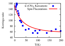
Figure 5: [Color online] Comparison of the spin fluctuation theory with the measuredkawamoto:kcn3 temperature dependence of the nuclear spin relaxation rate per unit temperature, $1/T_{1}T$ (left panel), Knight shift, $K_{s}$ (center panel), and Korringa ratio (right panel) of the Mott insulating phase of $\kappa$-(ET)₂Cu₂(CN)₃ [abbreviated as $\kappa$-(CN)₃ in the keys to the figures]. The spin fluctuation model is in good agrement with the measured $1/T_{1}T$, but does not describe the Knight shift (and hence $\cal K$) well. We have also checked that using the Fermi liquid for $\chi_{\mathrm{LW}}$ does not improve the fit to the $K_{s}$ data, and this fit is shown as a dashed line. This fit to the data is clearly worse than simply setting $\chi_{\mathrm{LW}}=0$. Also note that the peak in $1/T_{1}T$, $T_{\mathrm{NMR}}$, is at a lower temperature than the maximum in the Knight shift, $T_{K_{s}}$. This behavior is qualitatively different from that of the other $\kappa$ salts where $T_{\mathrm{NMR}}\sim T_{K_{s}}$ (see Figs. 1 and 4). This suggests that in $\kappa$-(ET)₂Cu₂(CN)₃ the origin of the $1/T_{1}T$ suppression is different from physics that gives rise to the maximum in $K_{s}$. The parameter values from the lines of best fit shown in this figure are reported in Table 2. The fact that the model gives a reasonably good fit to $1/T_{1}T$ but not to the $K_{s}$ data suggests that the spin fluctuation model fails to correctly account for the long wavelength physics, but suggests that the model correctly describes the physics around a peak in $\chi({\bf q},\omega)$ which dominates the integral over the first Brillouin zone and thus $1/T_{1}T$ [c.f., Eq. (2a)]. This is rather surprising as the correlation length is less than one lattice constant at $T=50$ K. This result is clearly inconsistent with the initial assumption that the long wavelength susceptibility is dominated by a peak in the dynamic susceptibility at a finite wave vector. Finally we note that the fact that ${\cal K}>1$ shows that the spin fluctuations are antiferromagnetic, this is rather interesting given the importance of Nagaoka ferromagnetism on the triangular lattice.nacoo

The NMR relaxation rate in $\kappa$-(ET)₂Cu₂(CN)₃ (Ref. kawamoto:kcn3 and Fig. 5) shows a similar temperature dependence to that in, for example, $\kappa$-(ET)₂Cu[N(CN)₂]Br. $1/T_{1}T$ is enhanced over the Korringa-like behavior with a peak at $T_{\mathrm{NMR}}\sim 10$ K below which it exhibits a large decrease. However the Knight shift $K_{s}$ in $\kappa$-(ET)₂Cu₂(CN)₃ is quite different to that in $\kappa$-(ET)₂Cu[N(CN)₂]Br (compare Figs. 4 and 5). In $\kappa$-(ET)₂Cu₂(CN)₃, $K_{s}$ increases as the temperature is lowered from room temperature until it reaches a broad maximum around $T_{K_{s}}\sim 30-50$ K below which it drops rapidly. In contrast, $K_{s}$ in $\kappa$-(ET)₂Cu[N(CN)₂]Br shows a weak temperature dependence down to $T_{K_{s}}$ below which it undergoes a sharp decrease (see Fig. 4). Another difference is $T_{\mathrm{NMR}}$ is considerably lower than $T_{K_{s}}$ in $\kappa$-(ET)₂Cu₂(CN)₃ whereas they are roughly the same in $\kappa$-(ET)₂Cu[N(CN)₂]Br. This suggests that whereas the suppression of $1/T_{1}T$ below $T_{\mathrm{NMR}}$ and $K_{s}$ below $T_{K_{s}}$ in $\kappa$-(ET)₂Cu[N(CN)₂]Br probably has a common origin; in $\kappa$-(ET)₂Cu₂(CN)₃ the origin of the suppression of $1/T_{1}T$ below $T_{\mathrm{NMR}}$ is different from the origin of the broad maximum in $K_{s}$ at $T_{K_{s}}$. Note that the fact that ${\cal K}>1$ shows that the spin fluctuations are antiferromagnetic, this is rather interesting given the importance of Nagaoka ferromagnetism on the triangular lattice.nacoo

Given the reasonable agreement between the antiferromagnetic spin fluctuation model with the NMR data on $\kappa$-(ET)₂Cu[N(CN)₂]Br (down to $T_{\mathrm{NMR}}\sim 50$ K), we apply the same formalism to $\kappa$-(ET)₂Cu₂(CN)₃. A slight modification to the spin fluctuation model is necessary since, unlike the other $\kappa$ salts studied in this paper, $\kappa$-(ET)₂Cu₂(CN)₃ is an insulator. Therefore we clearly cannot use the Fermi liquid form of $\chi_{\mathrm{LW}}$. The simplest approximation is that the dynamic susceptibility given in Eq. (3) will only consist of $\chi_{\mathrm{AF}}({\bf q},\omega)$. In the region where $\xi(T)/a$ is large, $\chi_{Q}=\alpha(\xi/a)^{2-\eta}$ and $\omega_{\mathrm{SF}}=\alpha^{\prime}(\xi/a)^{-z}$ where $\alpha$ and $\alpha^{\prime}$ are temperature independent constants and $a$ is the lattice spacing. Within these approximations the nuclear spin relaxation rate and Knight shift are given by

$$\frac{1}{T_{1}T} = \left(\frac{1}{T_{1}T}\right)_{0}\frac{(\xi/a)^{2+z-\eta}}{1+(Qa)^{2}(\xi/a)^{2}}$$

$$K_{s} = (K_{s})_{0}\frac{(\xi/a)^{2-\eta}}{1+(Qa)^{2}(\xi/a)^{2}}$$ (19)

with

$$\left(\frac{1}{T_{1}T}\right)_{0} = \frac{2\alpha k_{B}|A|^{2}}{\alpha^{\prime}\gamma_{e}^{2}\hbar^{4}}$$

$$(K_{s})_{0} = \frac{\alpha^{\prime}|A|}{\gamma_{e}\gamma_{N}\hbar^{2}},$$ (20)

where ${\bf Q}=(Q,Q)$ is the finite wave vector on which we assume the susceptibility to peak. Again, we take the temperature dependence of the correlation length to be $\xi(T)/\xi(T_{x})=\sqrt{2T_{x}/(T+T_{x})}$.

Following the same approximation scheme as before (outlined in Section II B), we assume a relaxational dynamics of the spin fluctuations, which are described by a dynamic critical exponent $z=2$, and a mean field critical exponent $\eta=0$. Within these approximations $\omega_{\mathrm{SF}}=\alpha(a/\xi)^{2}$ and $\chi_{Q}=\alpha^{\prime}(\xi/a)^{2}$. The nuclear spin relaxation rate and Knight shift are then given by

$$\frac{1}{T_{1}T} = \frac{(1/T_{1}T)_{0}C^{2}}{(T/T_{x}+1)^{2}+(Qa)^{2}C(T/T_{x}+1)}$$

$$K_{s} = \frac{(K_{s})_{0}C}{1+(Qa)^{2}C+T/T_{x}}.$$ (21)

We work in the high temperature approximation for $1/T_{1}T$ - following a procedure similar to that employed to obtain Eq. (15b). If the dynamic susceptibility is strongly peaked at $q=Q$ then the parameter $2(Qa)^{2}(\xi(T_{x})/a)^{2}$ is much larger than 1 so $(Qa)^{2}C(T/T_{x}+1)$ is larger than $(T/T_{x}+1)^{2}$ and we can just keep the term proportional to $(Qa)^{2}$ in the denominator which allows us to write $1/T_{1}T$ as

$$\frac{1}{T_{1}T}\simeq\frac{(1/T_{1}T)_{0}[\sqrt{2}\xi(T_{x})/a]^{2}}{(Qa)^{2}(T/T_{x}+1)}$$ (22)

We use the expressions for $1/T_{1}T$ given in Eq. (22) and for $K_{s}$ in Eq. (21) to fit the $\kappa$-(ET)₂Cu₂(CN)₃ data.kawamoto:kcn3 We assume the susceptibility has a strong peak at $Q=2\pi/3$. The parameters of the best fit are reported in Table 2 and the results are plotted in Fig 5. While the spin fluctuation model produces a reasonably good fit to the $1/T_{1}T$ above $T_{\mathrm{NMR}}\sim 10$ K, it does not reproduce $K_{s}$ data well as can be seen from the upward curvature in the fit in contrast to the data which shows a slight downward curvature. We also performed the fit to $\kappa$-(ET)₂Cu₂(CN)₃ data using the most general forms Eq. (19) and taking $z$ and $\eta$ as free parameters. Good fits to $1/T_{1}T$ and $K_{s}$ can be obtained with $\eta\sim 1$ and $z\sim 2$ but this gives us so many free parameters that the value of such fits must be questioned.

An important fact is that $K_{s}$ probes the long wavelength dynamics. We have set $\chi_{\mathrm{LW}}(\omega)$ to zero in order to make the simplest possible assumption about the insulating state. The data indicate that this assumption is probably incorrect. Recently Zheng et al.zheng used a high temperature series expansion to calculate the uniform spin susceptibility (which is the same as the Knight shift apart from a constant of proportionality) for the Heisenberg model on a triangular lattice, applied it to $\kappa$-(ET)₂Cu₂(CN)₃. They obtained a good agreement with the experimental data. The spin fluctuation model described here can be viewed as a different route to understand the same experiment. The discrepancy between the spin fluctuation model and the data suggests a failure of our implicit assumption that the long wavelength physics, which determines $K_{s}$, is dominated by a peak in the dynamic susceptibility due to spin fluctuations. This is consistent with the fact that we find that $\xi(T)\sim 0.2-0.4$ lattice spacings at $T=50$ K which clearly disagrees with our initial assumption that $\xi(T)\gg a$. This begs the question what physics dominates the long wavelength physics both in the series expansions and in the real material?

Parameter			Fit results
$(1/T_{1}T)_{0}$ $(s^{-1}$K-1)			220 $\pm 11$
$(K_{s})_{0}$			8100 $\pm$ 720
$T_{x}$ (K)			40 $\pm$ 4
$\xi(T_{x})/a$			0.3 $\pm$ 0.1

Table 2: The parameters obtained from the best fits to $1/T_{1}T$ and $K_{s}$ data in $\kappa$-(ET)₂Cu₂(CN)₃. These parameters are used to produce Fig. 5. The antiferromagnetic correlation length $\xi(T_{x})/a$ is short ranged consistent with the significant frustrationshimizu; zheng; zheng2 present in this material.

The low temperature properties of $\kappa$-(ET)₂Cu₂(CN)₃ are clearly inconsistent with a magnetic ordered ground state. For a two-dimensional quantum spin system with an ordered ground state, the low temperature properties are captured by the non-linear sigma model. The observed temperature dependence of $1/T_{1}$ and the spin echo rate $1/T_{2}$ follow $1/T_{1}\propto T^{7/2}\xi(T)$, and $1/T_{2}\propto T^{3}\xi(T)$, where the correlation length $\xi(T)$ is given bychubukov

$$\frac{\xi(T)}{a}=0.021\left(\frac{c}{\rho_{s}}\right)\left(\frac{4\pi\rho_{s}}{T}\right)^{1/2}\exp\left(\frac{4\pi\rho_{s}}{T}\right)$$ (23)

where $c$ is the spin wave velocity and $\rho_{s}$ is the spin stiffness. In the quantum critical regime,chubukov $1/T_{1}T\sim T^{\eta-1}$ and $1/T_{2}\sim T^{\eta-1}$ [c.f., Eq. (12)] where $\eta$ is the anomalous critical exponent associated with the spin-spin correlation function whose value is generally less than 1. Thus for a magnetically ordered state, which can be well described by O(N) non linear sigma model, both $1/T_{1}T$ and $1/T_{2}$ should increase with decreasing temperature. For $\kappa$-(ET)₂Cu₂(CN)₃ Shimizu et al.shimizu2 found that $1/T_{1}T\sim T^{1/2}$ and $1/T_{2}\sim$ constant from 1 K down to 20 mK which suggests the critical exponent $\eta>1$. The nuclear spin relaxation rate decreases with decreasing temperature. Such a large value of $z$ is what occurs for deconfined spinons.chubukov

V Unconventional Coherent Transport Regime and the $\kappa$-(ET)${}_{2}X$ Phase Diagram

In Section II.2, we discussed the DMFT description of the crossover from a bad metal to a Fermi liquid. DMFT successfully predicts the unconventional behaviors observed in a number of experiments on the $\kappa$-(ET)${}_{2}X$ salts. These include the resistivity, thermopower, and ultrasound velocity. The unconventional behaviors seen in these measurements are associated with the crossover from bad metallic regime to a renormalized Fermi liquid in the DMFT picture. While DMFT gives reliable predictions for the transport properties,Jaime-HH-DMFT; merino; limelette; hassan it is not able to explain the loss of DOS observed in the nuclear spin relaxation rate and Knight shift. Thus the NMR data suggest that the coherent transport regime is not simply a Fermi liquid, contrary to what has previously been thought.

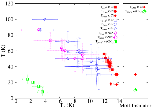
Figure 6: [Color online] The relationship between different temperature scales for a range of organic charge transfer salts. The superconducting transition temperature $T_{c}$ is used to parameterize the proximity of the material to the Mott transition ($T_{\mathrm{c}}$ decreases as one moves further away from the Mott transition). A plot of $T_{\rho\sim T^{2}},T_{\Delta v/v},$ and $T_{\mathrm{NMR}}$ against $T_{\mathrm{c}}$ for several $\kappa$-(ET)${}_{2}X$  salts shows that the peak in $1/T_{1}T$, $T_{\mathrm{NMR}}$, occurs at the same temperature as the crossover form a bad metal to the coherent transport regime measured in transport ($T_{\rho\sim T^{2}}$) and ultrasonic attenuation ($T_{\Delta v/v}$) experiments. $T_{\rho\sim T^{2}}$ is the temperature at which the resistivity deviates from a $T^{2}$ behavior, $T_{\Delta v/v}$ is the temperature at which a dip in the ultrasound velocity is observed. The left panel shows the data for the $\kappa$-(ET)${}_{2}X$ family in the metallic phase {$\kappa$-(ET)₂Cu[N(CN)₂]Cl and $\kappa$-(ET)₂Cu₂(CN)₃ under pressure, $\kappa$-(ET)₂Cu[N(CN)₂]Br and $\kappa$-(ET)₂Cu(NCS)₂} while the right panel shows the data for the $\kappa$-(ET)${}_{2}X$ family in the insulating phase [$\kappa$-(ET)₂Cu[N(CN)₂]Cl and $\kappa$-(ET)₂Cu₂(CN)₃ at ambient pressure]. In the metallic phase we use $T_{c}$ as a single parameter to characterize the effect of chemical substitution and hydrostatic pressure. This works surprisingly well and the data for $\kappa$-(ET)₂Cu[N(CN)₂]Cl, $\kappa$-(ET)₂Cu[N(CN)₂]Br, and $\kappa$-(ET)₂Cu(NCS)₂  is seen to collapse roughly onto a single trend, which suggests that the spin fluctuations in the metallic phases are rather similar. In contrast, the data for $\kappa$-(ET)₂Cu₂(CN)₃ fall onto a separate curve which suggests that there are important differences between the spin fluctuations in this material and those in other $\kappa$ phase salts. This is perhaps not so surprising in light of the fact that $\kappa$-(ET)₂Cu₂(CN)₃ has a spin liquid round state in its Mott insulating phase while the materials are close to at Néel ordered Mott insulating phase. This plot suggests that the pseudogap opens at the same temperature as the crossover from bad metal to coherent transport regime. Whether this is because of a deep link between the crossover and the pseudogap or because the lack of coherence in the bad metal destroys the pseudogap remains to be seen. Collectively these data show that the coherent transport regime is not simply a renormalised Fermi liquid as has previously been thought. It should be emphasized that the large error bars are the result of our estimates of the systematic errors produced by equating pressures in different experiments. The procedure to obtain the error bars presented in this plot is discussed in Appendix C. The symbols represent both the material and the experiment as follows: filled symbols correspond to the data for $\kappa$-(ET)₂Cu[N(CN)₂]Cl, open symbols denote $\kappa$-(ET)₂Cu[N(CN)₂]Br, open symbols with black dots denote $\kappa$-(ET)₂Cu(NCS)₂, and half filled symbols denote $\kappa$-(ET)₂Cu₂(CN)₃. The square symbols represent $T_{\rho\sim T^{2}}$ vs $T_{\mathrm{c}}$, circles represent $T_{\Delta v/v}$ vs $T_{\mathrm{c}}$, and triangles represent $T_{\mathrm{NMR}}$ vs $T_{\mathrm{c}}$. The references from which the data were collected are given in Table 3.

Material	$T_{\mathrm{c}}(P)$	$T_{\rho\sim T^{2}}(P)$	$T_{\Delta v/v}(P)$	$T_{\mathrm{NMR}}(P)$
$\kappa$-Cl	[lefebvre; fournier]	[limelette]	[fournier]	[lefebvre]
$\kappa$-Br	[frikach; schirber]	[strack]	[frikach]	[mayaffre]
$\kappa$-NCS	[caulfield]	-	[frikach]	[kawamoto]
$\kappa$-(CN)3	[kurosaki]	[kurosaki]	-	[kawamoto:kcn3]

Table 3: The references from which the pressure dependence of different temperature scales for different materials used to produce Fig. 6 were taken. The notation is the same as that given in Fig. 6. $T_{\rho\sim T^{2}}$ is the temperature at which the resistivity deviates from a $T^{2}$ behavior, $T_{\Delta v/v}$ is the temperature at which a dip in the ultrasound velocity is observed, and $T_{\mathrm{NMR}}$ is the temperature on which $1/T_{1}T$ peaks. In the table $\kappa$-Cl, $\kappa$-Br, and $\kappa$-NCS and $\kappa$-(CN)₃ are used as shorthand for $\kappa$-(ET)₂Cu[N(CN)₂]Cl, $\kappa$-(ET)₂Cu[N(CN)₂]Br, $\kappa$-(ET)₂Cu(NCS)₂, and $\kappa$-(ET)₂Cu₂(CN)₃ respectively.

To illustrate the nature of the low temperature paramagnetic metallic state more qualitatively, it is instructive to study how the bad metal-coherent transport crossover is related to the loss of DOS. Therefore we have investigated the relationship between $T_{\rho\sim T^{2}}$, the temperature at which the resistivity deviates from $T^{2}$ behavior; $T_{\Delta v/v}$, the temperature at which a dip in the ultrasonic velocity is observed; and $T_{\mathrm{NMR}}$, the temperature at which $1/T_{1}T$ (and $K_{s}$) is maximum which appears to mark the onset of a loss of DOS. In Figure 6 we plot $T_{\rho\sim T^{2}}$, $T_{\Delta v/v}$, and $T_{\mathrm{NMR}}$ as measured by several different groups for various salts against $T_{\mathrm{c}}$ which serves well as a single parameter to characterize both the hydrostatic pressure and the variation in chemistry (or ‘chemical pressure’). This analysis is complicated by the necessity of comparing pressures from different experiments. Our procedure for dealing with this issue is outlined in the Appendix C, and we stress that the large error bars in Fig. 6 are due to the difficulties in accurately measuring pressure rather than problems in determining $T_{c}$, $T_{\rho\sim T^{2}}$, $T_{\Delta v/v}$, or $T_{\mathrm{NMR}}$.

It is clear from Fig. 6 that the data for $\kappa$-(ET)₂Cu[N(CN)₂]Cl, $\kappa$-(ET)₂Cu[N(CN)₂]Br, and $\kappa$-(ET)₂Cu(NCS)₂  fall roughly onto a single curve. This suggests that $T_{\mathrm{NMR}}$ coincides with $T_{\rho\sim T^{2}}$ and $T_{\Delta v/v}$. Thus the loss of DOS, associated with $T_{\mathrm{NMR}}$, occurs around the temperature at which the crossover from bad metal to coherent transport regime takes place. The loss of DOS observed in $1/T_{1}T$ and $K_{s}$ is not what one would expect for a Fermi liquid; therefore the coherent intralayer transport regime is more complicated than a renormalized Fermi liquid. This must result from non-local correlations which are not captured by DMFT since DMFT captures local correlations exactly. One possible explanation for the loss of DOS is the opening of a pseudogap.

Another important point to emphasize from Fig. 6 is the appearance of a second trend formed by $\kappa$-(ET)₂Cu₂(CN)₃ which is clearly distinct from the trend of the data points from $\kappa$-(ET)₂Cu[N(CN)₂]Cl, $\kappa$-(ET)₂Cu[N(CN)₂]Br, and $\kappa$-(ET)₂Cu(NCS)₂. This shows that the spin fluctuations in $\kappa$-(ET)₂Cu₂(CN)₃ are qualitatively different from those in the other $\kappa$-(ET)${}_{2}X$ salts. Of course, qualitative differences are not entirely unexpected due to the spin liquid rather than antiferromagnetic ground state in $\kappa$-(ET)₂Cu₂(CN)₃. It has recently been argued that the differences in the spin fluctuations in $\kappa$-(ET)₂Cu₂(CN)₃ will lead this material to display a superconductivity with a different symmetry of the order parameter than the other $\kappa$-(ET)${}_{2}X$ salts.ben:d+id; powell:group This result shows that the spin fluctuations are indeed qualitatively different in $\kappa$-(ET)₂Cu₂(CN)₃.

On the basis of the above analysis we sketch the phase diagram of $\kappa$-(ET)${}_{2}X$, shown in Fig. 3. The pseudogap phase shows an interesting set of behaviors. On one hand it exhibits a loss of DOS as is evident from $1/T_{1}T$ and $K_{s}$. On the other hand, it exhibits coherent intralayer transport as is shown by the $T^{2}$ resistivity behaviorlimelette; it also has long lived quasiparticles and a well defined Fermi surface clearly seen from de Haas-van Alphen and Shubnikov-de Haas oscillation experiments.wosnitza; singleton; kartsovnik One framework in which it may be possible to understand both of these sets of behaviors is if there is a fluctuating superconducting gap.scarratt This idea has been applied to the cuprates;schmalian1; schmalian2 it would be interesting to see whether such an approach gives a good description of $\kappa$-(ET)${}_{2}X$. Another interesting observation is that the measurements which see the loss in the DOS probe the spin degrees of freedom whereas the evidence for well defined quasiparticles comes from probes of the charge degrees of freedom. This may be suggestive of a ‘spin gap’ which could result from singlet formation as in the RVB picture.

To date there have been few experiments studying the pressure dependence of $1/T_{1}T$ or $K_{s}$. Therefore it is not possible, at present, to determine with great accuracy where the pseudogap vanishes. The available NMR experiment under pressuremayaffre; wzietek-review suggest that at sufficiently high pressures the pseudogap onset temperature is lower than the incoherent-coherent crossover temperature and pressure eventually suppresses the pseudogap altogether. We represent the current uncertainty over where the pseudogap is completely suppressed by pressure by drawing a shaded area with a question mark in the phase diagram. It is plausible that the pseudogap vanishes very close, if not at the same pressure, to the point where the superconducting gap vanishes. This would be consistent with RVB calculationsben:prl; zhang which suggest that the pseudogap and superconducting gap are proportional to each other and so should vanish at about the same pressure. However, we should stress that there really is not yet sufficient data to determine exactly where the pseudogap vanishes and admit that our choice is, perhaps, a little provocative.

Clearly a series of careful experiments are required to elucidate when $T_{\mathrm{NMR}}$ tends to zero. Understanding where the pseudogap vanishes is an important consideration in light of the number of theories based on a hidden pseudogap quantum critical point in the cuprates.Sachdev Furthermore, the superconducting state in organic charge transfer salts far from the Mott transition are highly unconventional. These low $T_{c}$ organic charge transfer salts have unexpectedly large penetration depthsujjual; pratt and are not described by BCS theory.constraints The possibility that a quantum critical point is associated with the pressure where $T_{c}$ goes to zero invites comparison with the heavy fermion material CeCoIn_5-xSn_x CeCoIn in which a quantum critical point seems to be associated with the critical doping to suppress superconductivity. Thus low $T_{c}$ organic charge transfer salts appear increasingly crucial for our understanding of the organic charge transfer salts.powell:review

An important question to address theoretically is why $T_{\mathrm{NMR}}$ might coincide with $T_{\rho\sim T^{2}}$ and $T_{\Delta v/v}$. Of course, it may be that the two phenomena are intimately connected. However, another possibility suggests itself on the basis of DMFT and RVB calculations. DMFT correctly captures the local physics and it is this local physics that dominates the cross-over from a ‘bad-metal’ to coherent in-plane transport. On the other hand RVB does not capture this cross-over (because the Mott transition is only dealt with at the Brinkmann-Rice levelbrinkman) but does capture some of the non-local physics which DMFT neglects. The pseudogap is predicted by RVB theory to increase in temperature when pressure is lowered.ben:prl; zhang This rise in the pseudogap temperature is predicted to continue until the pressure is lowered all the way to the Mott transition, in contrast with the observed behavior (c.f., Figs 3 and 6). However, we conjecture that the RVB physics is ‘cut off’ by the loss of coherence at $T_{\rho\sim T^{2}}$ and $T_{\Delta v/v}$ thus preventing $T_{\mathrm{NMR}}$ from exceeding $T_{\rho\sim T^{2}}\approx T_{\Delta v/v}$.

VI Conclusions

We have applied a spin fluctuation model to study the temperature dependences of the nuclear spin relaxation rate and Knight shift in the paramagnetic metallic phases of several quasi two-dimensional organic charge transfer salts. The large enhancement of $1/T_{1}T$ between $T_{\mathrm{NMR}}$ {$\sim 50$ K in $\kappa$-(ET)₂Cu[N(CN)₂]Br} and room temperature has been shown to be the result of strong antiferromagnetic spin fluctuations. The antiferromagnetic correlation length is estimated to be $3.5\pm 2.5$ lattice spacings in $\kappa$-(ET)₂Cu[N(CN)₂]Br at $T=50$ K. The temperature dependence of $1/T_{1}T$ for $T\textgreater T_{\mathrm{NMR}}$ from the spin fluctuation model is qualitatively similar with the predictions of DMFT. The spin fluctuations in $\kappa$-(ET)₂Cu[N(CN)₂]Cl, $\kappa$-(ET)₂Cu[N(CN)₂]Br, $\kappa$(d8)-(ET)₂Cu[N(CN)₂]Br, and $\kappa$-(ET)₂Cu(NCS)₂ are found to be remarkably similar both qualitatively and quantitatively. Strong spin fluctuations seem to be manifested in materials close to Mott transition. Recent NMR experimentskawamoto:ag on $\kappa$-(ET)₂Ag(CN)${}_{2}\cdot$H₂O, which is situated further away from the Mott transition, suggests that the spin fluctuations in this materials are not as strong as those in the other $\kappa$ salts studied here.

We have also applied the spin fluctuation formalism to the strongly frustrated system $\kappa$-(ET)₂Cu₂(CN)₃. In this compound the measured $1/T_{1}T$, which probes the entire Brillouin zone, agrees well with the predictions of the spin fluctuation model for $T>T_{\mathrm{NMR}}\sim 10$ K. In contrast the measured Knight shift, which only depends on the long wavelength physics, is not well described by the spin fluctuation model. This suggests that at least one of the assumptions made in the spin fluctuation model: (i) $z=2$, $\eta=0$, or (ii) $\chi({\bf q},\omega)$ is strongly peaked at wave vector ${\bf q}={\bf Q}$; is violated in $\kappa$-(ET)₂Cu₂(CN)₃ or that the model neglects some important long wavelength physics. In light of the recent evidence for a spin liquid ground state in $\kappa$-(ET)₂Cu₂(CN)₃, in contrast to the antiferromagnetic or ‘$d$-wave’ superconducting grounds states in $\kappa$-(ET)₂Cu[N(CN)₂]Cl, $\kappa$-(ET)₂Cu[N(CN)₂]Br, $\kappa$(d8)-(ET)₂Cu[N(CN)₂]Br, and $\kappa$-(ET)₂Cu(NCS)₂, and the greater degree of frustration in $\kappa$-(ET)₂Cu₂(CN)₃ it is interesting that there are such important qualitative and quantitative differences between the spin fluctuations in $\kappa$-(ET)₂Cu₂(CN)₃ and those in the other $\kappa$ phase salts.

The peak of $1/T_{1}T$ and the suppression of $K_{s}$ are strongly dependent on pressure: they are systematically reduced and completely vanish at high pressure (> 4 kbar);mayaffre at high pressure a Korringa-like temperature dependences of $1/T_{1}T$ and $K_{s}$ are recovered for all temperatures. It is clear that high pressures will suppress both the antiferromagnetic spin fluctuations which are dominant above 50 K and the mechanism (presumably the pseudogap) which causes drops in $1/T_{1}T$ and $K_{s}$ below 50 K at ambient pressure.

The large suppression of $1/T_{1}T$ and $K_{s}$ below $T_{\mathrm{NMR}}$ observed in all the $\kappa$ salts studied here cannot be explained by the M-MMP spin fluctuation model. The most plausible mechanism to account for this feature is the appearance of a pseudogap which causes the suppression of the density of states at the Fermi energy. This is because at low temperature $1/T_{1}T$ and $K_{s}$ are proportional $\tilde{\rho}^{2}(E_{F})$ and $\tilde{\rho}(E_{F})$, respectively [c.f., Eq. (LABEL:nmr_correlated)]. Independent evidence for the suppression of density of states at the Fermi level comes from the linear coefficient of specific heat $\gamma$.timusk The electronic specific heat probes the density of excitations within $k_{B}T$ of the Fermi energy. Any gap will suppress the density of states near the Fermi surface which results in the depression of the specific heat coefficient $\gamma$. Kanodakanoda:jspj2006 compared $\gamma$ for several of the $\kappa$-(ET)${}_{2}X$ salts and found that in the region close to the Mott transition, $\gamma$ is indeed reduced. One possible interpretation of this behavior is a pseudogap which becomes bigger as one approaches the Mott transition. However, other interpretations are also possible, in particular one needs to take care to account for the coexistence of metallic and insulating phases; this is expected as the Mott transition is first order in the organic charge transfer salts.kagawa; sasaki The existence of a pseudogap has also been suggested $\lambda$-(BEDT-TSF)₂GaCl₄suzuki from microwave conductivity. The reduction of the real part of the conductivity $\sigma_{1}$ from the Drude conductivity $\sigma_{\mathrm{dc}}$ and the steep upturn in the imaginary part of the conductivity $\sigma_{2}$ may be interpreted in term of preformed pairs leading to a pseudogap in this material.

The experimental evidence from measurements of $1/T_{1}T$, $K_{s}$, and heat capacity all seem to point to the existence of a pseudogap below $T_{\mathrm{NMR}}$ in $\kappa$-(ET)₂Cu[N(CN)₂]Br and $\kappa$-(ET)₂Cu(NCS)₂. Thus a phenomenological description which takes into account both the spin fluctuations which are important above $T_{\mathrm{NMR}}$ and a pseudogap which dominates the physics below $T_{\mathrm{NMR}}$ would seem to be a reasonable starting point to explain the NMR data for the entire temperature range (clearly superconductivity must also be included for $T<T_{\mathrm{c}}$). We will pursue this approach in our future work. In particular one would like to answer the following questions: how big is the pseudogap and what symmetry does it have? Is there any relation between the pseudogap and the superconducting gap? The answer to these questions may help put constraints on the microscopic theories.

Future experiments. There are a number of key experiments to study the pseudogap. The pressure and magnetic field dependences of the nuclear spin relaxation rate and Knight shift will be valuable in determining the pseudogap phase boundary, estimating the order of magnitude of the pseudogap, and addressing the issue how the pseudogap is related to superconductivity. In the cuprates, there have been several investigations of the magnetic field dependence of the pseudogap seen in NMR experiments. For Bi₂Sr_1.6La_0.4CuO₆ the nuclear spin relaxation rate does not change will field up to 43 T.gqzheng2 However, since $T^{*}\sim 200$ K, one may require a larger field to reduce the pseudogap. Similar results were found in YBa₂Cu₄O₈.gqzheng However, in YBa₂Cu₃O_7-δ [see especially Fig. 6 of Ref. mitrovic] a field of order 10 T is enough to start to close the pseudogap. Mitrovic et al.mitrovic interpret this observation in terms of the suppression of ‘$d$-wave’ superconducting fluctuations.

The interlayer magnetoresistance of the cuprates has proven to a sensitive probe of the pseudogap. mozorov; shibauchi; kawakami; elbaum Moreover, it is found that for the field perpendicular to the layers (which means that Zeeman effects will dominate orbital magnetoresistance effects) the pseudogap is closed at a field given by

$$H_{PG}\simeq\frac{\hbar k_{B}T^{*}}{\gamma_{e}}$$ (24)

where $T^{*}$ is the pseudogap temperature. For the hole doped cuprates this field is of the order $\sim 100$ T. In contrast, for the electron-doped cuprates this field is of the order $\sim 30$ T (and $T^{*}\sim 30-40$ K), and so this is much more experimentally accessible.kawakami The field and temperature dependence of the interlayer resistance for several superconducting organic charge transfer saltszuo is qualitatively similar to that for the cuprates. In particular, for temperatures less than the zero-field transition temperature and fields larger than the upper critical field, negative magnetoresistance is observed for fields perpendicular to the layers. A possible explanation is that, as in the cuprates, there is a suppression of the density of states near the Fermi energy, and the associated pseudogap decreases with increasing magnetic field.

A Nernst experiment can be used to probe whether there are superconducting fluctuations in the pseudogap phase, as has been done in the cuprates.wang This experiment is particularly important in understanding the relation between the pseudogap and superconductivity.

One could also study the pressure dependence of the linear coefficient of heat capacity $\gamma$. Since $\gamma$ is proportional to the density of states at the Fermi energy, a detailed mapping of $\gamma(P)$ would be an important probe for the study the pseudogap. Finally, measurements of the Hall effect have also led to important insights into the pseudogap of the cupratestimusk therefore perhaps the time is ripe to revisit these experiments in the organic charge transfer salts.

Appendix A Vertex corrections and the dynamic spin susceptibility for Strongly Correlated Electrons

We consider a strongly interacting electron system and derive the real and imaginary parts of the dynamic susceptibility. We show that under some quite general (but specific) conditions that the Korringa ratio is unity. Many definitions are simply stated in this appendix since most are derived more fully in any number of textbooks (for example Ref. Mahan). The general expression for the dynamic susceptibility in Matsubara formalism is given by

$$\chi_{\alpha\beta}({\bf q},i\omega_{n})=\int_{0}^{\beta}{d\tau e^{i\omega_{n}\tau}\langle T_{\tau}m_{\alpha}({\bf q},\tau)m_{\beta}(-{\bf q},0)\rangle},$$ (25)

where $\beta=1/k_{B}T$ is the inverse temperature, $\tau$ is the imaginary time, $\omega_{n}=(2n+1)\pi k_{B}T/\hbar$ is the Matsubara frequency, $m_{\alpha}$ is the component of magnetization in the $\alpha$ direction, and $T_{\tau}$ is the (imaginary) time ordering operator. In order to consider $\chi_{-+}({\bf q},\omega)$ we define the operators:

$$m_{-}({\bf q},\tau) = \frac{\hbar\gamma_{e}}{\sqrt{2}}\sum_{{\bf p}}c_{{\bf p}+{\bf q},\downarrow}^{\dagger}(\tau)c_{{\bf p},\uparrow}(\tau),$$ (26)

$$m_{+}({\bf q},\tau) = \frac{\hbar\gamma_{e}}{\sqrt{2}}\sum_{{\bf p}}c_{{\bf p}+{\bf q},\uparrow}^{\dagger}(\tau)c_{{\bf p},\downarrow}(\tau).$$ (27)

Upon substituting (26) and (27) into (25) and performing the appropriate Wick contractions on the operators one finds that

$$\chi_{-+}({\bf q},i\omega_{n})=\frac{\hbar^{2}\gamma_{e}^{2}}{2}\int_{0}^{\beta}{d\tau e^{i\omega_{n}\tau}\Gamma({\bf p}+{\bf q},-\tau;{\bf p},\tau)}$$

$$\times G({\bf p}+{\bf q},-\tau)G({\bf p},\tau)$$ (28)

where $\Gamma({\bf q},\tau;{\bf p},\tau^{\prime})$ is the vertex function, $G({\bf p},ip_{n})$ is the full interacting Green’s function given by

$$G({\bf p},\tau)=\frac{G_{0}({\bf p},\tau)}{1-G_{0}({\bf p},\tau)\Sigma({\bf p},\tau)},$$ (29)

$G^{0}({\bf p},\tau)$ is the non interacting Green’s function, and $\Sigma({\bf p},\tau)$ is the self energy. The $\tau$ integration can be evaluated by first transforming the integrand in Eq. (28) into momentum space. This gives

$$\chi_{-+}({\bf q},i\omega_{n}) = \frac{\hbar^{2}\gamma_{e}^{2}}{2\beta}\sum_{{\bf p},ip_{m}}\Gamma({\bf p}+{\bf q},ip_{m};{\bf p},ip_{m}+i\omega_{n})$$ (30)

$$\times G({\bf p}+{\bf q},ip_{m})G({\bf p},ip_{m}+i\omega_{n})$$

where $\Gamma({\bf q},i\omega_{n};{\bf p},i\omega_{n}^{\prime})$ is the Fourier transform of $\Gamma({\bf q},\tau;{\bf p},\tau^{\prime})$ and $G({\bf p},ip_{n})$ given by

$$G({\bf p},ip_{n})=\frac{1}{ip_{n}-\varepsilon_{\bf p}-\Sigma({\bf p},ip_{n})},$$ (31)

where $\varepsilon_{\bf p}$ is the dispersion of the non-interacting system. To evaluate the Matsubara summation, it is convenient to express the full interacting Green’s function using the spectral representation

$$G({\bf p},ip_{n})=\int_{-\infty}^{\infty}{\frac{dE_{1}}{2\pi}\frac{A_{s}({\bf p},E_{1})}{ip_{n}-E_{1}}},$$ (32)

where $A_{s}({\bf p},E_{1})$ is the spectral function given by

$$A_{s}({\bf p},E)=\frac{-2\mathrm{Im}\Sigma({\bf p},E)}{(E-\varepsilon_{\bf p}-\mathrm{Re}\Sigma({\bf p},E))^{2}+(\mathrm{Im}\Sigma({\bf p},E))^{2}}.$$ (33)

Substituting (32) into (30), the dynamic susceptibility becomes

$$\chi_{-+}({\bf q},i\omega_{n}) = \frac{\hbar^{2}\gamma_{e}^{2}}{2\beta}\sum_{{\bf p},m}\int_{-\infty}^{\infty}\frac{dE_{1}}{2\pi}\frac{dE_{2}}{2\pi}$$

$$\times\Gamma({\bf p}+{\bf q},ip_{m};{\bf p},ip_{m}+i\omega_{n})$$

$$\times\frac{A_{s}({\bf p}+{\bf q},E_{1})A_{s}({\bf p},E_{2})}{(ip_{m}-E_{1})(ip_{m}+i\omega_{n}-E_{2})}.$$

At this stage we neglect vertex corrections, that is we set $\Gamma({\bf p}+{\bf q},ip_{n};{\bf p},ip_{n}+i\omega_{n})=1$ for all ${\bf p}$, ${\bf q}$, $p_{n}$, and $\omega_{n}$. After performing the Matsubara sum and analytical continuation $i\omega_{n}\to\omega+i\eta$, the dynamic susceptibility is given by

$$\chi_{-+}({\bf q},\omega) = \frac{\hbar^{2}\gamma_{e}^{2}}{2}\sum_{{\bf p}}\int_{-\infty}^{\infty}\frac{dE_{1}}{2\pi}\frac{dE_{2}}{2\pi}A_{s}({\bf p}+{\bf q},E_{1})$$ (35)

$$\times A_{s}({\bf p},E_{2})\frac{n_{F}(E_{1})-n_{F}(E_{2})}{\hbar\omega+E_{1}-E_{2}+i\eta},$$

where $n_{F}(E)$ is the Fermi function.

First we discuss the imaginary part of $\chi_{-+}({\bf q},\omega)$. Using the well known relation $1/(x+i\eta)=P(1/x)-i\pi\delta(x)$, where $P(y)$ denotes the principal value, the imaginary part of $\chi_{-+}({\bf q},i\omega_{n})$ in the limit of small frequency $\omega$ is given by

$$\lim_{\omega\to 0}\frac{\chi^{\prime\prime}_{-+}({\bf q},\omega)}{\omega}$$

$$=\frac{\hbar^{2}\gamma_{e}^{2}}{2}\sum_{{\bf p}}\int_{-\infty}^{\infty}\frac{dE}{4\pi}A_{s}({\bf p}+{\bf q},E)A_{s}({\bf p},E)\left(-\frac{\partial n_{F}}{\partial E}\right).$$

(36)

The nuclear spin relaxation rate is obtained by summing the dynamic susceptibility over all q [c.f., Eq. (2a)] thus we find that

$$\frac{1}{T_{1}T} = \frac{k_{B}|A|^{2}}{\hbar}\int_{-\infty}^{\infty}\frac{dE}{4\pi}\sum_{{\bf p}}\sum_{{\bf q}}A_{s}({\bf p},E)A_{s}({\bf p}+{\bf q},E)$$ (37)

$$\times\left(-\frac{\partial n_{F}}{\partial E}\right),$$

where we have assumed a contact, i.e. momentum independent, hyperfine coupling. This expression can be written in the more intuitive form

$$\frac{1}{T_{1}T}=\frac{k_{B}|A|^{2}}{\hbar}\int_{-\infty}^{\infty}\frac{dE}{4\pi}\tilde{\rho}^{2}(E)\left(-\frac{\partial n_{F}}{\partial E}\right),$$ (38)

where

$$\tilde{\rho}(E)=\sum_{\bf p}A_{s}({\bf p},E)$$ (39)

is the full interacting density of states. At temperatures small enough so that $\tilde{\rho}(E)$ varies little with energy within $k_{B}T$ of the Fermi energy, $E_{F}$, the expression can be further simplified to

$$\frac{1}{T_{1}T}\simeq\frac{k_{B}|A|^{2}\tilde{\rho}^{2}(E_{F})}{4\pi\hbar}.$$ (40)

Within the approximation of neglecting vertex corrections the real part of the dynamic susceptibility is given by

$$\chi^{\prime}({\bf q},\omega) = \frac{\hbar^{2}\gamma_{e}^{2}}{2}\sum_{{\bf p}}\int_{-\infty}^{\infty}\frac{dE_{1}}{2\pi}A_{s}({\bf p}+{\bf q},E_{1})$$ (41)

$$\times\int_{-\infty}^{\infty}\frac{dE_{2}}{2\pi}F({\bf p},E_{1},E_{2},\omega,T)$$

with

$$F({\bf p},E_{1},E_{2},\omega,T)=\frac{A_{s}({\bf p},E_{2})[n_{F}(E_{1})-n_{F}(E_{2})]}{\hbar\omega+E_{1}-E_{2}}.$$ (42)

To perform the integration over $E_{2}$, we first make the change of variable $x=\omega+E_{1}-E_{2}$ and take the limit $\omega\to 0$. Thus the integral over $E_{2}$ becomes

$$\int_{-\infty}^{\infty}\frac{dx}{2\pi}F({\bf p},E_{1},x,\omega,T)$$

$$=-\int_{-\infty}^{\infty}\frac{dx}{2\pi}A_{s}({\bf p},E_{1}-x)\frac{n_{F}(E_{1})-n_{F}(E_{1}-x)}{x}$$

$$=\left(-\frac{dn_{F}}{dE_{1}}\right)\int_{-\infty}^{\infty}\frac{dx}{2\pi}A_{s}({\bf p},E_{1}-x).$$ (43)

By using sum rule

$$\int_{-\infty}^{\infty}\frac{dy}{2\pi}A_{s}({\bf p},y)=1,$$ (44)

$\chi^{\prime}_{-+}({\bf q},0)$ then becomes

$$\chi^{\prime}_{-+}({\bf q},0)=\frac{\hbar^{2}\gamma_{e}^{2}}{2}\int_{-\infty}^{\infty}\frac{dE}{2\pi}\sum_{{\bf p}}A_{s}({\bf p}+{\bf q},E)\left(-\frac{\partial n_{F}}{\partial E}\right)$$

. (45)

The Knight shift is obtained by setting ${\bf q}=\bf 0$ [c.f., Eq. (2c)] and is

$$K_{s}=\frac{|A|\gamma_{e}}{2\gamma_{N}}\int_{-\infty}^{\infty}\frac{dE}{2\pi}\tilde{\rho}(E)\left(-\frac{\partial n_{F}}{\partial E}\right).$$ (46)

At temperatures sufficiently low that $\tilde{\rho}(E)$ varies little with energy within $k_{B}T$ near the Fermi energy, the Knight shift is given by

$$K_{s}\simeq\frac{|A|\gamma_{e}\tilde{\rho}(E_{F})}{4\pi\gamma_{N}}.$$ (47)

Using Eqs. (40) and (47), the Korringa ratio for interacting electrons with a contact hyperfine coupling and neglecting vertex corrections is

$$\mathcal{K} = \frac{\hbar}{4\pi k_{B}}\left(\frac{\gamma_{e}}{\gamma_{N}}\right)^{2}\frac{1}{T_{1}TK_{s}^{2}}$$ (48)

$$= \frac{\hbar}{4\pi k_{B}}\left(\frac{\gamma_{e}}{\gamma_{N}}\right)^{2}\frac{k_{B}|A|^{2}\tilde{\rho}^{2}(E_{F})}{4\pi\hbar}\left(\frac{4\pi\gamma_{N}}{|A|\gamma_{e}\tilde{\rho}(E_{F})}\right)^{2}$$

$$= 1.$$

For non interacting electrons, the self energy $\Sigma({\bf q},\omega)=0$; expressions Eqs. (38) and (46) are still valid and one only need replace $\tilde{\rho}(E)$ with the non interacting density of states $\rho(E)$. On the temperature scale over which the density of states varies little with energy, the Korringa ratio for free electron gas ${\cal K}_{\mathrm{free}}=1$. By comparing Eqs. (48) and ${\cal K}_{\mathrm{free}}=1$ we see that any deviation of the Korringa ratio from one must be caused by either vertex corrections or the q-dependence of the hyperfine coupling.

Appendix B Estimation of effect of thermal expansion of the lattice on the Knight shift

In this appendix we describe how we obtained our estimates of the isothermal compressibility the linear coefficient of thermal expansion and the pressure dependence of the Knight shift. By feeding these estimates into Eq. (III.4) we estimate the correction to the Knight shift required because measurements are generally performed at constant pressure whereas calculations are most naturally performed at constant volume. The difference between these two versions of the Knight shift can be quite significant as can be seen in Fig. 4.

First, let us discuss the first term in the integrand in Eq. (III.4). We observed that $K_{s}^{p}$ can be rewritten as $K_{s}^{p}=[\hbar\gamma_{e}^{2}/(4\pi k_{B}\gamma_{N}^{2}T_{1}T{\cal K})]^{1/2}$. Using Mayaffre’s data,mayaffre we extracted the pressure dependence of $1/T_{1}T$ at constant temperature and estimated that $(1/T_{1}T)^{1/2}$ is roughly linear with pressure: $(1/T_{1}T)^{1/2}\sim-3$x$10^{-5}P$ for $T_{1}$ in second, $T$ in Kelvin, and $P$ in bar. We then used this result and the Korringa value for non interacting electron gas to calculate $\left(\partial K_{s}^{p}/\partial P\right)_{T}$ for $\kappa$-(ET)₂Cu[N(CN)₂]Br which is found to be around $-3$x$10^{-8}$/bar. One can compare the value obtained here with $\left(\partial K_{s}^{p}/\partial P\right)_{T}$ obtained from the pressure dependence study on effective mass in $\kappa$-(ET)₂Cu(NCS)₂ compoundcaulfield which is presumably more reliable. Since $K_{s}$ should be proportional to the effective mass, the quantity of interest $\left(\partial K_{s}^{p}/\partial P\right)_{T}$ can be estimated from the pressure dependence of the effective mass data which yields a value around $-6$x$10^{-8}$/bar. The two estimates agree to with a factor of two.

Next we need to obtain a value for lattice isothermal compressibility. We use the analytical expression obtained from DMFThassan

$$(\mathscr{K}v)^{-1}=\frac{B_{0}}{v_{0}}-\left(\frac{\nu D_{0}}{v_{0}}\right)^{2}\chi_{\mathrm{el}},$$ (49)

where $\mathscr{K}$ is the inverse isothermal compressibility $(v\partial P/\partial v)^{-1}$, $v_{0}$ is the reference unit-cell volume, $v$ is the unit-cell volume under pressure, $B_{0}$ is a reference bulk elastic modulus, $D_{0}$ is a reference bandwidth, $\nu$ is a parameter that characterizes the change in the bandwidth under pressure, and $\chi_{\mathrm{el}}$ is the electronic susceptibility. We estimated that for $\kappa$-(ET)₂Cu[N(CN)₂]Cl, $v_{0}=1700~{}\AA^{3}$, $B_{0}=122$ kbar, $D_{0}=0.13$ eV, and $D_{0}\chi_{\mathrm{el}}\sim 1$. Putting everything together, the order of magnitude of the lattice isothermal compressibility for $\kappa$-(ET)₂Cu[N(CN)₂]Cl is around $-10^{5}$ bar. Although we are not aware of any measurements of the isothermal compressibility of $\kappa$-(ET)₂Cu[N(CN)₂]Cl  systematic axial pressure studieskondo on $\alpha$-(BEDT-TTF)NH₄Hg(NCS)₄ found that the isothermal compressibility is of order $-10^{5}$ bar, a value which is very close to our crude estimate for $\kappa$-(ET)₂Cu[N(CN)₂]Cl.

The temperature dependence of the thermal expansion at constant pressure has been measured by Müller et al.muller:lattice They found that $\kappa$-(ET)₂Cu[N(CN)₂]Cl, $\kappa$-(ET)₂Cu(NCS)₂, and undeuterated and fully deuterated $\kappa$-(ET)₂Cu[N(CN)₂]Br all have a relatively temperature independent thermal expansion above about 80 K while complicated features are observed below 80 K associated with glassy transitions and the many-body behavior of these materials. Since we are only interested in getting an order of magnitude, we neglect the complicated temperature dependence observed in $\kappa$-(ET)₂-X and approximate the thermal expansion as a constant. The value extracted from Müller et al.’s data is around $10^{-4}$ K^-1.

Appendix C Estimation of Errors in Figure 6

In this appendix we outline the procedure use to estimate the errors on the data presented in Fig 6. Let us consider a given set of data, for example $T_{\mathrm{c}}(P)$. To a reasonable degree of accuracy, $T_{\mathrm{c}}$ for $\kappa$-(ET)${}_{2}X$  decreases linearly with increasing pressure, i.e. $T_{\mathrm{c}}=aP+b$ where $a$ and $b$ are the coefficients obtained from fitting the expression to the data. In a typical pressure measurement, there will be some uncertainties in the pressure ($\Delta P$) which may be caused by systematic errors due to the uncertainties in the pressure calibration. The size of $\Delta P$ will depend on a specific apparatus used in the experiment. For example, a helium gas pressure system would have uncertainties as large as 0.1 kbar while a clamped pressure cell which uses oil pressure medium may have uncertainties as large as 1 kbar.murata; graf Knowing $\Delta P$, we can estimate the uncertainty in $T_{\mathrm{c}}$ when it is compared with another data set from a different experiment taken by a different group, say $T_{\rho\sim T^{2}}(P)$. This is done by calculating the following:

$$\Delta T_{\mathrm{c}}=\frac{dT_{\mathrm{c}}(P)}{dP}\Delta P.$$ (50)

Another way to estimate $\Delta T_{\mathrm{c}}$ is to calculate $dT_{\mathrm{c}}(P)/dP$ from the discontinuity in the thermal expansion and specific heat by using the Ehrenfest relation.muller:sm These two methods give similar results. For $\kappa$-(ET)₂Cu[N(CN)₂]Br, $dT_{\mathrm{c}}(P)/dP$ is estimated to be around $-2.4$ K/kbar from the first method while it is found to be around $-2.2$ K/kbar from the Ehrenfest relation. This procedure is repeated for other data sets, $T_{\rho\sim T^{2}}(P)$, $T_{\Delta v/v}(P)$, and $T_{\mathrm{NMR}}(P)$ whenever applicable which leads to $T_{\mathrm{c}}\pm\Delta T_{\mathrm{c}}$, $T_{\rho\sim T^{2}}\pm\Delta T_{\rho\sim T^{2}}$, $T_{\Delta v/v}\pm\Delta T_{\Delta v/v}$, and $T_{\mathrm{NMR}}\pm\Delta T_{\mathrm{NMR}}$. We then tabulate $T_{\rho\sim T^{2}},T_{\Delta v/v},$ and $T_{\mathrm{NMR}}$ with respect to $T_{\mathrm{c}}$ for a given pressure. The results are shown in Fig 6. In some cases we were not able to obtain a reasonable fit because either the data are very scattered or there are not enough data to perform fit. This is the reason for the absence of error bars on the vertical axis for some data points in Fig 6.

References

- P. A. Lee, N. Nagaosa, and X.-G. Wen (2006) P. A. Lee, N. Nagaosa, and X.-G. Wen, Rev. Mod. Phys. 78, 17 (2006).
- E. Dagotto, T. Hotta, and A. Moreo (2003) E. Dagotto, T. Hotta, and A. Moreo, Phys. Rep. 344, 1 (2003).
- (3) F. Esch, S. Fabris, L. Zhou, T. Montini, C. Africh, P. Fornasiero, G. Comelli, and R. Rosei, Science 309, 752 (2005), and references therein.
- K. Takada, H. Sakurai, E. T.-Muromachi, F. Izumi, R. A. Dilanian, and T. Sasaki (2003) K. Takada, H. Sakurai, E. T.-Muromachi, F. Izumi, R. A. Dilanian, and T. Sasaki, Nature 422, 53 (2003).
- A.P. Mackenzie and Y. Maeno (2003) A.P. Mackenzie and Y. Maeno, Rev. Mod. Phys. 75, 657 (2003).
- S. A. Grigera, P. Gegenwart, R. A. Borzi, F. Weickert, A. J. Schofield, R. S. Perry, T. Tayama, T. Sakakibara, Y. Maeno, A. G. Green, A. P. Mackenzie (2004) S. A. Grigera, P. Gegenwart, R. A. Borzi, F. Weickert, A. J. Schofield, R. S. Perry, T. Tayama, T. Sakakibara, Y. Maeno, A. G. Green, A. P. Mackenzie, Science 306, 1154 (2004).
- Stewart (1984) G. R. Stewart, Rev. Mod. Phys. 56, 755 (1984).
- Powell and McKenzie (2006) B. J. Powell and R. H. McKenzie, J. Phys.: Condens. Matter 18, R827 (2006).
- C. H. Pennington and V. A. Stenger (1996) C. H. Pennington and V. A. Stenger, Rev. Mod. Phys. 68, 855 (1996).
- V. F. Mitrović, E. E. Sigmund, M. Eschrig, H. N. Bachman, W. P. Halperin, A. P. Reyes, P. Kuhns, W. G. Moulton (2001) V. F. Mitrović, E. E. Sigmund, M. Eschrig, H. N. Bachman, W. P. Halperin, A. P. Reyes, P. Kuhns, W. G. Moulton, Nature 413, 501 (2001).
- V. A. Sidorov, M. Nicklas, P. G. Pagliuso, J. L. Sarrao, Y. Bang, A. V. Balatsky, and J. D. Thompson (2002) V. A. Sidorov, M. Nicklas, P. G. Pagliuso, J. L. Sarrao, Y. Bang, A. V. Balatsky, and J. D. Thompson, Phys. Rev. Lett. 89, 157004 (2002).
- Miyagawa et al. (2004) K. Miyagawa, K. Kanoda, and A. Kawamoto, Chem. Rev. 104, 5635 (2004).
- M. R. Norman, contribution to The Handbook of Magnetism and Advanced Magnetic Materials (2006) (Eds. H. Kronmuller and S. Parkin) M. R. Norman, contribution to The Handbook of Magnetism and Advanced Magnetic Materials (Eds. H. Kronmuller and S. Parkin), vol. 5 (Wiley, 2006), cond-mat/0609559.
- R. H. McKenzie (1995) R. H. McKenzie, Phys. Rev. Lett. 74, 5140 (1995).
- N. Mannella, W. L. Yang, X. J. Zhou, H. Zheng, J. F. Mitchell, J. Zaanen, T. P. Devereaux, N. Nagaosa, Z. Hussain, Z.-X. Shen (2005) N. Mannella, W. L. Yang, X. J. Zhou, H. Zheng, J. F. Mitchell, J. Zaanen, T. P. Devereaux, N. Nagaosa, Z. Hussain, Z.-X. Shen, Nature 438, 474 (2005).
- A. Yeh, Y.-A. Soh, J. Brooke, G. Aeppli, T. F. Rosenbaum, and S. M. Hayden (2002) A. Yeh, Y.-A. Soh, J. Brooke, G. Aeppli, T. F. Rosenbaum, and S. M. Hayden, Nature 419, 459 (2002).
- Ishiguro et al. (2001) T. Ishiguro, K. Yamaji, and G. Saito, Organic Superconductors (Springer, Berlin, 2001).
- Mayaffre et al. (1994) H. Mayaffre, P. Wzietek, D. Jérome, C. Lenoir, and P. Batail, Europhys. Lett. 25, 208 (1994).
- S. M. De Soto et al. (1995) S. M. De Soto, C. P. Slichter, A. M. Kini, H. H. Wang, U. Geiser, and J. M. Williams, Phys. Rev. B 52, 10364 (1995).
- Miyagawa et al. (2002) K. Miyagawa, A. Kawamoto, and K. Kanoda, Phys. Rev. Lett. 89, 017003 (2002).
- Kawamoto et al. (1995) A. Kawamoto, K. Miyagawa, Y. Nakazawa, and K. Kanoda, Phys. Rev. Lett. 74, 3455 (1995).
- F. Gebhard (1997) F. Gebhard, The Mott Metal-Insulator Transition, (Springer, Berlin, 1997).
- M. Imada, A. Fujimori, and Y. Tokura (1998) M. Imada, A. Fujimori, and Y. Tokura, Rev. Mod. Phys. 70, 1039 (1998).
- Merino and McKenzie (2000a) J. Merino and R. H. McKenzie, Phys. Rev. B 61, 7996 (2000a).
- P. Limelette, P. Wzietek, S. Florens, A. Georges, T. A. Costi, C. Pasquier, D. Jérome, C. Mézière, and P. Batail (2003) P. Limelette, P. Wzietek, S. Florens, A. Georges, T. A. Costi, C. Pasquier, D. Jérome, C. Mézière, and P. Batail, Phys. Rev. Lett. 91, 016401 (2003).
- F. Kagawa, K. Miyagawa, and K. Kanoda (2005) F. Kagawa, K. Miyagawa, and K. Kanoda, Nature 436, 534 (2005).
- F. Kagawa, T. Itou, K. Miyagawa, and K. Kanoda (2004) F. Kagawa, T. Itou, K. Miyagawa, and K. Kanoda, Phys. Rev. Lett. 93, 127001 (2004).
- Greedan (2001) J. E. Greedan, J. Mater. Chem. 11, 37 (2001).
- N. P. Ong and R. J. Cava (2004) N. P. Ong and R. J. Cava, Science 305, 5680 (2004).
- Merino et al. (2006) J. Merino, B. J. Powell, and R. H. McKenzie, Phys. Rev. B 73, 235107 (2006).
- Shimizu et al. (2003) Y. Shimizu, K. Miyagawa, K. Kanoda, M. Maesato, and G. Saito, Phys. Rev. Lett. 91, 107001 (2003).
- Tamura and Kato (2002) M. Tamura and R. Kato, J. Phys.: Condens. Matter 14, L729 (2002).
- Nakamura et al. (2001) T. Nakamura, T. Takahashi, S. Aonuma, and R. Kato, J. Mater. Chem. 11, 2159 (2001).
- Hassan et al. (2005) S. R. Hassan, A. Georges, and H. R. Krishnamurthy, Phys. Rev. Lett. 94, 036402 (2005).
- Merino and McKenzie (2000b) J. Merino and R. H. McKenzie, Phys. Rev. B 62, 16442 (2000b).
- R. C. Yu, J. M. Williams, H. H. Wang, J. E. Thompson, A. M. Kini, K. D. Carlson, J. Ren, M.-H. Whangbo, and P. M. Chaikin (1991) R. C. Yu, J. M. Williams, H. H. Wang, J. E. Thompson, A. M. Kini, K. D. Carlson, J. Ren, M.-H. Whangbo, and P. M. Chaikin, Phys. Rev. B 44, 6932 (1991).
- Frikach et al. (2000) K. Frikach, M. Poirier, M. Castonguay, and K. D. Truong, Phys. Rev. B 61, R6491 (2000).
- Fournier et al. (2003) D. Fournier, M. Poirier, M. Castonguay, and K. D. Truong, Phys. Rev. Lett. 90, 127002 (2003).
- For a review see J. Singleton (2000) For a review see J. Singleton, Rep. Prog. Phys. 63, 1111 (2000).
- Wosnitza (1996) J. Wosnitza, Fermi surfaces of low-dimensional organic metals and superconductors (Springer, Berlin-New York, 1996).
- Kartsovnik (2004) M. V. Kartsovnik, Chem. Rev. 104, 5737 (2004).
- Timusk and Statt (1999) T. Timusk and B. Statt, Rep. Prog. Phys. 62, 61 (1999).
- M. R. Norman, D. Pines, and C. Kallin (2005) M. R. Norman, D. Pines, and C. Kallin, Adv. Phys. 54, 715 (2005).
- Moriya and Ueda (2000) T. Moriya and K. Ueda, Adv. Phys. 49, 555 (2000).
- A.J. Millis, H. Monien, and D. Pines (1990) A.J. Millis, H. Monien, and D. Pines, Phys. Rev. B 42, 167 (1990).
- Schmalian (1998) J. Schmalian, Phys. Rev. Lett. 81, 4232 (1998).
- Kino and Kontani (1998) H. Kino and H. Kontani, J. Phys. Soc. Jpn. 67, 3691 (1998).
- Jujo et al. (1999) T. Jujo, S. Koikegami, and K. Yamada, J. Phys. Soc. Jpn. 68, 1331 (1999).
- Powell and McKenzie (2005) B. J. Powell and R. H. McKenzie, Phys. Rev. Lett. 94, 047004 (2005).
- For a review see K. Kuroki (2006) For a review see K. Kuroki, J. Phys. Soc. Jpn. 75, 051013 (2006).
- Kanoda (2006) K. Kanoda, J. Phys. Soc. Jpn. 75, 051007 (2006).
- Pratt et al. (2003) F. L. Pratt, S. J. Blundell, I. M. Marshall, T. Lancaster, S. L. Lee, A. Drew, U. Divakar, H. Matsui, and N. Toyota, Polyhedron 22, 2307 (2003).
- Pratt and Blundell (2005) F. L. Pratt and S. J. Blundell, Phys. Rev. Lett. 94, 097006 (2005).
- Powell and McKenzie (2004a) B. J. Powell and R. H. McKenzie, J. Phys.: Condens. Matter 16, L367 (2004a).
- Liu et al. (2005) J. Liu, J. Schmalian, and N. Trivedi, Phys. Rev. Lett. 94, 127003 (2005).
- Gan et al. (2005) J. Y. Gan, Y. Chen, Z. B. Su, and F. C. Zhang, Phys. Rev. Lett. 94, 067005 (2005).
- (57) B. J. Powell and R. H. McKenzie, cond-mat/0607079, to appear in Phys. Rev. Lett.
- Anderson et al. (2004) P. W. Anderson, P. A. Lee, M. Randeria, T. M. Rice, N. Trivedi, and F. C. Zhang, J. Phys.: Condens. Matter 16 (2004).
- J. G. Analytis, A. Ardavan, S. J. Blundell, R. L. Owen, E. F. Garman, C. Jeynes, and B. J. Powell (2006) J. G. Analytis, A. Ardavan, S. J. Blundell, R. L. Owen, E. F. Garman, C. Jeynes, and B. J. Powell, Phys. Rev. Lett. 96, 177002 (2006).
- Powell and McKenzie (2004b) B. J. Powell and R. H. McKenzie, Phys. Rev. B 69, 024519 (2004b).
- Powell (2006) B. J. Powell, J. Phys.: Condens. Matter 18, L575 (2006).
- Zhang et al. (1988) F. C. Zhang, C. Gros, T. M. Rice, and H. Shiba, Supercond. Sci. Technol. 1, 36 (1988).
- V. Barzykin and D. Pines, Phys. Rev. B52, 13585 ; 96, 247002 (2006)() (1995) V. Barzykin and D. Pines, Phys. Rev. B52, 13585 (1995); 96, 247002 (2006).
- (64) C. M. Varma, P. B. Littlewood, S. Schmitt-Rink, E. Abrahams, and A. E. Ruckenstein, Phys. Rev. Lett. 63, 1996 (1989); 64, 497(E) (1990).
- H. Monien, P. Monthoux, and D. Pines (1991) H. Monien, P. Monthoux, and D. Pines, Phys. Rev. B 43, 275 (1991).
- H. Monien, D. Pines, and M. Takigawa (1991) H. Monien, D. Pines, and M. Takigawa, Phys. Rev. B 43, 258 (1991).
- Moriya (1963) T. Moriya, J. Phys. Soc. Jpn. 18, 516 (1963).
- Narath and Weaver (1968) A. Narath and H. T. Weaver, Phys. Rev. 175, 373 (1968).
- A. Georges, G. Kotliar, W. Krauth, and M. J. Rozenberg (1996) A. Georges, G. Kotliar, W. Krauth, and M. J. Rozenberg, Rev. Mod. Phys. 68, 1 (1996).
- Kotliar and Vollhardt (2004) G. Kotliar and D. Vollhardt, Phys. Today 57, 53 (2004).
- Pruschke et al. (1995) T. Pruschke, M. Jarrell, and J. K. Freericks, Adv. Phys. 44, 187 (1995).
- M. Jarrell, J. E. Gubernatis, and R. N. Silver (1991) M. Jarrell, J. E. Gubernatis, and R. N. Silver, Phys. Rev. B 44, 5347 (1991).
- Chubukov et al. (1994) A. V. Chubukov, S. Sachdev, and T. Senthil, Nucl. Phys. B 426, 601 (1994).
- M. Takigawa, P. C. Hammel, R. H. Heffner, Z. Fisk, K. C. Ott, and J. D. Thompson (1989) M. Takigawa, P. C. Hammel, R. H. Heffner, Z. Fisk, K. C. Ott, and J. D. Thompson, Physica C 162-164, 853 (1989).
- N. Bulut, D. Hone, D. J. Scalapino, and N. E. Bickers (1990) N. Bulut, D. Hone, D. J. Scalapino, and N. E. Bickers, Phys. Rev. Lett. 64, 2723 (1990).
- K. Ishida, K. Okamoto, Y. Kawasaki, Y. Kitaoka, O. Trovarelli, C. Geibel, and F. Steglich (2002) K. Ishida, K. Okamoto, Y. Kawasaki, Y. Kitaoka, O. Trovarelli, C. Geibel, and F. Steglich, Phys. Rev. Lett. 89, 107202 (2002).
- J. Aarts, F. R. de Boer, and D. E. MacLaughlin (1983) J. Aarts, F. R. de Boer, and D. E. MacLaughlin, Physica 121B, 162 (1983).
- Y. Kitaoka, H. Arimoto, Y. Kohori, and K. Asayama (1985) Y. Kitaoka, H. Arimoto, Y. Kohori, and K. Asayama, J. Phys. Soc. Jpn. 54, 3236 (1985).
- K. Ishida, Y. Minami, Y. Kitaoka, S. Nakatsuji, N. Kikugawa, and Y. Maeno (2003) K. Ishida, Y. Minami, Y. Kitaoka, S. Nakatsuji, N. Kikugawa, and Y. Maeno, Phys. Rev. B 67, 214412 (2003).
- H.-Q. Ding and M. S. Makivic, Phys. Rev. Lett. 64, 1449 ; J.-K. Kim and M. Troyer, Phys. Rev. Lett. 80, 2705 (1998)() (1990) H.-Q. Ding and M. S. Makivic, Phys. Rev. Lett. 64, 1449 (1990); J.-K. Kim and M. Troyer, Phys. Rev. Lett. 80, 2705 (1998).
- Elstner et al. (1993) N. Elstner, R. R. P. Singh, and A. P. Young, Phys. Rev. Lett. 71, 1629 (1993).
- McKenzie (1998) R. H. McKenzie, Comments Cond. Matt. Phys. 18, 309 (1998).
- H. Taniguchi, R. Sato, K. Satoh, A. Kawamoto, H. Okamoto, T. Kobayasi and K. Mizuno (2006) H. Taniguchi, R. Sato, K. Satoh, A. Kawamoto, H. Okamoto, T. Kobayasi and K. Mizuno, J. Low. Temp. Phys. 142, 437 (2006).
- Wzietek et al. (1993) P. Wzietek, F. Creuzet, C. Bourbonnais, D. Jerome, K. Bechgaard, and P. Batail, J. Phys. I France 3, 171 (1993).
- A. Kawamoto, Y. Honma, and K. I. Kumagai (2004) A. Kawamoto, Y. Honma, and K. I. Kumagai, Phys. Rev. B 70, 060510(R) (2004).
- Kurosaki et al. (2005) Y. Kurosaki, Y. Shimizu, K. Miyagawa, K. Kanoda, and G. Saito, Phys. Rev. Lett. 95, 177001 (2005).
- Y. Shimizu, K. Miyagawa, K. Kanoda, M. Maesato, and G. Saito (2006) Y. Shimizu, K. Miyagawa, K. Kanoda, M. Maesato, and G. Saito, Phys. Rev. B 73, 140407(R) (2006).
- Zheng et al. (2005) W. Zheng, R. R. P. Singh, R. H. McKenzie, and R. Coldea, Phys. Rev. B 71, 134422 (2005).
- Motrunich (2005) O. I. Motrunich, Phys. Rev. B 72, 045105 (2005).
- S.-S. Lee and P. A. Lee (2005) S.-S. Lee and P. A. Lee, Phys. Rev. Lett. 95, 036403 (2005).
- (91) S.-S. Lee, P. A. Lee, and T. Senthil, cond-mat/0607105.
- Miyagawa et al. (1995) K. Miyagawa, A. Kawamoto, Y. Nakazawa, and K. Kanoda, Phys. Rev. Lett. 75, 1174 (1995).
- W. Zheng, J. O. Fjaerestad, R. R. P. Singh, R. H. McKenzie, and R. Coldea (2006) W. Zheng, J. O. Fjaerestad, R. R. P. Singh, R. H. McKenzie, and R. Coldea (2006).
- Shimizu et al. (2006) Y. Shimizu, K. Miyagawa, K. Kanoda, M. Maesato, and G. Saito, Phys. Rev. B 73, 140407(R) (2006).
- Lefebvre et al. (2000) S. Lefebvre, P. Wzietek, S. Brown, C. Bourbonnais, D. Jérome, C. Mézière, M. Fourmigué, and P. Batail, Phys. Rev. Lett. 85, 5420 (2000).
- J. E. Schirber, D. L. Overmyer, K. D. Carlson, J. M. Williams, A. M. Kini, H. H. Wang, H. A. Charlier, B. J. Love, D. M. Watkins, and G. A. Yaconi (1991) J. E. Schirber, D. L. Overmyer, K. D. Carlson, J. M. Williams, A. M. Kini, H. H. Wang, H. A. Charlier, B. J. Love, D. M. Watkins, and G. A. Yaconi, Phys. Rev. B 44, 4666 (1991).
- C. Strack, C. Akinci, V. Pashchenko, B. Wolf, E. Uhrig, W. Assmus, M. Lang, J. Schreuer, L. Wiehl, J. A. Schlueter, J. Wosnitza, D. Schweitzer, J. Müller, and J. Wykhoff (2005) C. Strack, C. Akinci, V. Pashchenko, B. Wolf, E. Uhrig, W. Assmus, M. Lang, J. Schreuer, L. Wiehl, J. A. Schlueter, J. Wosnitza, D. Schweitzer, J. Müller, and J. Wykhoff, Phys. Rev. B 72, 054511 (2005).
- Caulfield et al. (1994) J. Caulfield, W. Lubczynski, F. L. Pratt, J. Singleton, D. Y. K. Ko, W. Hayes, M. Kurmoo, and P. Day, J. Phys: Condens Matt. 6, 2911 (1994).
- R. H. McKenzie and D. Scarratt (1996) R. H. McKenzie and D. Scarratt, Phys. Rev. B 54, R12709 (1996).
- J. Schmalian, D. Pines, and B. Stojković (1998) J. Schmalian, D. Pines, and B. Stojković, Phys. Rev. Lett. 80, 3839 (1998).
- J. Schmalian, D. Pines, and B. Stojković (1999) J. Schmalian, D. Pines, and B. Stojković, Phys. Rev. B 60, 667 (1999).
- P. Wzietek, H. Mayaffre, D. Jérome and S. Brazovskii (1996) P. Wzietek, H. Mayaffre, D. Jérome and S. Brazovskii, J. Phys. I France 6, 2011 (1996).
- Sachdev (2003) S. Sachdev, Rev. Mod. Phys. 75, 913 (2003).
- Bauer et al. (2005) E. D. Bauer, C. Capan, F. Ronning, R. Movshovich, J. D. Thompson, and J. L. Sarrao, Phys. Rev. Lett. 94, 047001 (2005).
- W. F. Brinkman and T. M. Rice (1970) W. F. Brinkman and T. M. Rice, Phys. Rev. B 2, 4302 (1970).
- A. Kawamoto, Y. Honma, K. Kumagai, K. Yamamoto, and K. Yakushi (2006) A. Kawamoto, Y. Honma, K. Kumagai, K. Yamamoto, and K. Yakushi, J. Low Temp. Phys. 142, 519 (2006).
- T. Sasaki, N. Yoneyama, A. Suzuki, N. Kobayashi, Y. Ikemoto and H. Kimura (2005) T. Sasaki, N. Yoneyama, A. Suzuki, N. Kobayashi, Y. Ikemoto and H. Kimura, J. Phys. Soc. Jpn. 74, 2351 (2005).
- T. Suzuki, E. Negishi, H. Uozaki, H. Matsui, and N. Toyota (2006) T. Suzuki, E. Negishi, H. Uozaki, H. Matsui, and N. Toyota, J. Low Temp. Phys. 142, 567 (2006).
- G.-Q. Zheng, P. L. Kuhns, A. P. Reyes, B. Liang, and C. T. Lin (2005) G.-Q. Zheng, P. L. Kuhns, A. P. Reyes, B. Liang, and C. T. Lin, Phys. Rev. Lett. 94, 047006 (2005).
- G.-Q. Zheng, W. G. Clark, Y. Kitaoka, K. Asayama, Y. Kodama, P. Kuhns, and W. G. Moulton (1999) G.-Q. Zheng, W. G. Clark, Y. Kitaoka, K. Asayama, Y. Kodama, P. Kuhns, and W. G. Moulton, Phys. Rev. B 60, R9947 (1999).
- V. F. Mitrović, H. N. Bachman, W. P. Halperin, A. P. Reyes, P. Kuhns, and W. G. Moulton (2002) V. F. Mitrović, H. N. Bachman, W. P. Halperin, A. P. Reyes, P. Kuhns, and W. G. Moulton, Phys. Rev. B 66, 014511 (2002).
- N. Morozov, L. Krusin-Elbaum, T. Shibauchi, L. N. Bulaevskii, M. P. Maley, Yu. I. Latyshev, and T. Yamashita (2000) N. Morozov, L. Krusin-Elbaum, T. Shibauchi, L. N. Bulaevskii, M. P. Maley, Yu. I. Latyshev, and T. Yamashita, Phys. Rev. Lett. 84, 1784 (2000).
- Shibauchi et al. (2001) T. Shibauchi, L. Krusin-Elbaum, M. Li, M. P. Maley, and P. H. Kes, Phys. Rev. Lett. 86, 5763 (2001).
- T. Kawakami, T. Shibauchi, Y. Terao, M. Suzuki, and L. Krusin-Elbaum (2005) T. Kawakami, T. Shibauchi, Y. Terao, M. Suzuki, and L. Krusin-Elbaum, Phys. Rev. Lett. 95, 017001 (2005).
- L. Krusin-Elbaum, G. Blatter, and T. Shibauchi (2004) L. Krusin-Elbaum, G. Blatter, and T. Shibauchi, Phys. Rev. B 69, 220506(R) (2004).
- Zuo et al. (1999) F. Zuo, J. A. Schlueter, and J. M. Williams, Phys. Rev. B 60, 574 (1999).
- Y. Wang, L. Li, and N. P. Ong (2006) Y. Wang, L. Li, and N. P. Ong, Phys. Rev. B 73, 024510 (2006).
- G. D. Mahan (2000) G. D. Mahan, Many-Particle Physics (Kluwer Academic/Plenum, New York, 2000), 3rd ed., chapter 3.
- Kondo et al. (2003) R. Kondo, S. Kagoshima, and M. Maesato, Phys. Rev. B 67, 134519 (2003).
- J. Müller, M. Lang, F. Steglich, J. A. Schlueter, A. M. Kini, and T. Sasaki (2002) J. Müller, M. Lang, F. Steglich, J. A. Schlueter, A. M. Kini, and T. Sasaki, Phys. Rev. B 65, 144521 (2002).
- K. Murata, M. Ishibashi, Y. Honda, N. A. Fortune, M. Tokumoto, N. Kinoshita, and H. Anzai (1990) K. Murata, M. Ishibashi, Y. Honda, N. A. Fortune, M. Tokumoto, N. Kinoshita, and H. Anzai, Solid State Commun. 76, 377 (1990).
- D. Graf, private communication (2006) D. Graf, private communication (2006).
- J. Müller, M. Lang, J. A. Schlueter, U. Geiser, and D. Schweitzer (2001) J. Müller, M. Lang, J. A. Schlueter, U. Geiser, and D. Schweitzer, Synth. Met. 120, 855 (2001).
- (124) J. Singleton, R. D. McDonald, and N. Harrison, cond-mat/0606492.