Influence of vibrational modes on the electronic properties of DNA

Abstract

We investigate the electron (hole) transport through short double-stranded DNA wires in which the electrons are strongly coupled to the specific vibrational modes (vibrons) of the DNA. We analyze the problem starting from a tight-binding model of DNA, with parameters derived from ab-initio calculations, and describe the dissipative transport by equation-of-motion techniques. For homogeneous DNA sequences like Poly- (Guanine-Cytosine) we find the transport to be quasi-ballistic with an effective density of states which is modified by the electron-vibron coupling. At low temperatures the linear conductance is strongly enhanced, but above the ‘semiconducting’ gap it is affected much less. In contrast, for inhomogeneous (‘natural’) sequences almost all states are strongly localized, and transport is dominated by dissipative processes. In this case, a non-local electron-vibron coupling influences the conductance in a qualitative and sequence-dependent way.

I Introduction

Transport measurements on DNA display a wide range of properties, depending on the measurement setup, the environment, and the specific molecule, with behavior ranging from insulating Braun et al. (1998) via semi-conducting Porath et al. (2000) to quasi-metallic Xu et al. (2004). The variance of experimental results as well as ab-initio calculations Starikov (2005) suggest that the environment and its influence via the vibrational modes (vibrons) of DNA are an important factor for the electronic transport properties of DNA wires.

Numerous recent articles addressed the electronic properties in a microscopic approach Asai (2004); Galperin et al. (2006); Gutierrez et al. (2005, ). Typically, the DNA is described within a tight-binding model for the electronic degrees of freedom with parameters either taken from ab-initio quantum chemistry simulations Voityuk et al. (2000); Starikov (2005); Senthilkumar et al. (2005) or motivated by a fit to experiments. The variance of qualitatively different tight-binding models is large, ranging from involved all-atomic representations to models where each base pair is represented by only a single orbital.

Several suggestions in the past stressed the importance of the environment and vibrational modes on the electron transfer Conwell and Rakhmanova (2000); Henderson et al. (1999) and transport Yoo et al. (2001); Troisi and Orlandi (2002). However, the vibrons have been treated so far only within very simple models, where specifically only a local electron-vibron coupling has been taken into account Gutierrez et al. (2005). If the coupling is sufficiently strong, this leads to the formation of polarons, i.e., a bound state of an electrons with a a lattice distortion. While these approaches are sufficient to describe the transition from elastic (quasi-ballistic) to inelastic (dissipative) transport they ignore the fact that the non-local electron-vibron coupling strength is comparable in magnitude to the local one Starikov (2005). Furthermore, as the non-local electron-vibron coupling leads effectively to a vibron-assisted hopping, the proper inclusion of this coupling can be important for transport through the inhomogeneous sequences of ‘natural’ DNA.

In this paper we study electron transport through double-stranded DNA wires strongly coupled, both locally and non-locally, to vibrational modes of the DNA. The DNA base pairs are represented by single tight-binding orbitals, with energies differing for Guanine-Cytosine (GC) and Adenine-Thymine (AT) pairs. The vibrational modes are also coupled to the surrounding environment (water or buffer solution) which we represent by a harmonic oscillator bath. This extension allows for dissipation of energy and opens the possibility of inelastic transport processes. We address the influence of specific DNA vibrational modes on transport in the frame of equation-of-motion techniques, with parameters motivated by ab-initio calculations Starikov (2005); Senthilkumar et al. (2005).

Our two main results are: 1) For homogeneous DNA sequences like Poly- (Guanine-Cytosine) wires the vibrons strongly enhance the linear conductance at low temperatures. At large bias the vibrons affect the conductance only weakly, which remains dominated by quasi-ballistic transport through extended electronic states. 2) For inhomogeneous (‘natural’) sequences almost all states are strongly localized, and transport is dominated by inelastic (dissipative) processes. In this case, the presence of a non-local electron-vibron coupling, leading to ‘vibron-assisted’ electron hopping’, influences the conductance in a qualitative and quantitative way.

The paper is organized as follows: in the following section we introduce the model and sketch briefly the techniques used to derive the transport properties. In Section III.1 we present our results for homogeneous DNA wires, while in Section III.2 we discuss a specific inhomogeneous DNA sequence, that has been studied in recent experiments. A summary is provided in Section IV. Details of the applied technique can be found in the Appendix A.

II Model and technique

Quantum chemistry calculations Artacho et al. (2003); Lewis et al. (2003) show that the highest occupied molecular orbital (HOMO) of a DNA base pair is located on the Guanine or Adenine, whereas the lowest unoccupied molecular orbital (LUMO) is located on the Thymine and Cytosine. Between HOMO and LUMO there is an energetic gap of approximately $2-3\,e\rm{V}$. Experimental evidence hints to the prevalence of hole transport through DNA. Given the energetic and spatial separation of HOMO and LUMO and considering sufficiently low bias voltage we can represent in a minimal model one base pair by a single tight-binding orbital.

We consider a DNA sequence with N base pairs, the first and last of which are coupled to semi-infinite metal electrodes. We further allow for a coupling to (in general multiple) vibrational modes, that can be excited by local and non-local coupling to the charge carriers on the DNA. These modes in turn are coupled to the environment. When later performing the numerical calculations we will restrict ourselves to a single vibrational mode of the DNA base pair, e.g., the ‘stretch’ mode Starikov (2005).

We thus arrive at the Hamiltonian $H=H_{\rm el}+H_{\rm vib}+H_{\rm el-vib}+H_{\rm L}+H_{\rm R}+H_{\rm T,L}+H_{\rm T,R}+H_{\rm bath}$ with

$$H_{\rm el} = \sum_{i}\epsilon_{i}a_{i}^{\dagger}a_{i}-\sum_{i,j;i\neq j}t_{ij}a_{i}^{\dagger}a_{j}$$

$$H_{\rm T,L}+H_{\rm T,R} = \sum_{n,k,i}\left[t_{in}^{r}c_{nr}^{\dagger}a_{i}+t_{in}^{r*}a_{i}^{\dagger}c_{nr}\right]$$

$$H_{\rm vib} = \sum_{\alpha}\omega_{\alpha}B_{\alpha}^{\dagger}B_{\alpha}$$

$$H_{\rm el-vib} = \sum_{\alpha}\sum_{i}\lambda_{0}\,a_{i}^{\dagger}a_{i}(B_{\alpha}+B_{\alpha}^{\dagger})$$ (1)

$$+ \sum_{\alpha}\sum_{i,j;i\neq j}\lambda_{ij}\,a_{i}^{\dagger}a_{j}(B_{\alpha}+B_{\alpha}^{\dagger})\;.$$

The index $r=\rm L,R$ describing left and right electrode. The term $H_{\rm el}$ describes the electrons in the DNA chain with operators $a_{i}^{{\dagger}},a_{i}$ in a single-orbital tight-binding representation with on-site energies $\epsilon_{i}$ of the base pairs and hopping $t_{ij}$ between neighbouring base pairs. Both on-site energies and hopping depend on the base pair sequence, e.g., the on-site energy of a Guanine-Cytosine base pair differs from the on-site energy of a Adenine-Thymine base pair. For the hopping matrix elements $t_{ij}$ we used the values calculated by Siebbeles et al.Senthilkumar et al. (2005) who studied intra- and inter-strand hopping between the bases in DNA-dimers by density functional theory (DFT). They computed direction-dependent values for all possible hopping matrix elements in such dimers. Adapting these results to our simplified model of base pairs we obtain the hopping elements denoted in table 1   .

5’-XY-3’(all in $e$V)
X$\diagdown$ Y G C A T G 0.119 0.046 -0.186 -0.048 C -0.075 0.119 -0.037 -0.013 A -0.013 -0.048 -0.038 0.122 T -0.037 -0.186 0.148 -0.038

Table 1: Hopping integrals $t_{ij}$ taken form Ref. Senthilkumar et al., 2005 and adapted to our model. The notation 5’-XY-3’ indicates the direction along the DNA strand (see e.g. Fig. 1b in Ref. Endres et al., 2004.)

The number in the G row and the A column denotes the hopping matrix element from a GC base pair to an AT base pair to its ‘right’ (to the 3’ direction), for example.

The terms $H_{\rm L/R}$ refer to the left and right electrodes. They are modeled by non-interacting electrons, described by operators $c_{k\,\rm L/R}^{{\dagger}},c_{k\,\rm L/R}$, with a flat density of states $\rho_{e}$ (wide band limit). The chemical details of the coupling between the DNA and the electrodes are not the focus of this work. For our purposes it is fully characterized by $H_{\rm T,L}+H_{\rm T,R}$, which leads to a level broadening of the base pair orbitals coupled to the electrodes characterized by the linewidths $\Gamma^{\rm L}$ and $\Gamma^{\rm R}$.

The vibronic degrees of freedom are described by $H_{\rm vib}$, with bosonic operators $B_{\alpha}$ and $B_{\alpha}^{\dagger}$ for the vibron mode with frequency $\omega_{\alpha}$. $H_{\rm el-vib}$ couples the electrons on the DNA to the vibrational modes, where $\lambda_{0}$ and $\lambda_{ij}$ are the strengths for the local and non-local electron-vibron coupling, respectively. We further restrict the non-local coupling terms to nearest neighbors, $\lambda_{ij}=\lambda_{1}\delta_{i,j=i\pm 1}$. Note that the vibron modes and their coupling to electrons is assumed independent of the base pairs involved, an approximation that is reasonable for some modes of interest, including the base pair stretch mode Starikov (2005). The strength of the electron-vibron coupling for various vibrational modes has been computed in Ref. Starikov, 2005 for homogeneous dimers and tetramers of AT and GC pairs. Here we consider also inhomogeneous sequences, for which the electron-vibron couplings are not known. As a model we take $\lambda_{0}$ and $\lambda_{1}$ as parameters, independent of the base pairs involved, for which we choose values in rough agreement with estimates for the ‘stretch’ mode of Ref. Starikov, 2005. This should be sufficient for a qualitative discussion of the effects that arise from the electron-vibron coupling in DNA.

The vibrons are coupled to the environment, the microscopic details of which do not matter. We model it by a harmonic oscillator bath $H_{\rm bath}$, whose relevant properties are summarized by its linear (‘Ohmic’) power spectrum (or spectral function) up to a high-frequency cut-off $\omega_{c}$Weiss (1999). The coupling of the vibrons to the bath changes the vibrons spectra from discrete (Einstein) modes to continuous spectra with a peak around the vibron frequency. Physically, the coupling to a bath allows for dissipation of electronic and vibronic energy. This dissipation is crucial for the stability of the DNA molecule in a situation where inelastic contributions to the current dissipate a substantial amount of power on the DNA itself.

As mentioned before we only consider a single vibrational mode when performing the numerical calculations. This vibrational mode with resonance frequency $\omega_{0}$ coupled to the bath is then described by a spectral density

$$D(\omega)=\frac{1}{\pi}\left(\frac{\eta(\omega)}{(\omega-\omega_{0})^{2}+\eta(\omega)^{2}}-\frac{\eta(\omega)}{(\omega+\omega_{0})^{2}+\eta(\omega)^{2}}\right)\,,$$ (2)

with a frequency dependent broadening $\eta(\omega)$ which arises from the vibron-bath coupling. For the ’Ohmic’ bath with weak vibron-bath coupling and cut-off $\omega_{c}$ we consider $\eta(\omega)=0.05\,\omega\,\theta(\omega_{c}-\omega)$. Mathematically the crossover from the discrete vibrational modes to a continuous spectrum of a single mode is done by substituting $\sum_{\alpha}\delta(\omega-\omega_{\alpha})\rightarrow\int d\omega D(\omega)$.

For the strong electron-vibron coupling predicted for DNAStarikov (2005), one expects polaron formation, with a polaron size of a few base pairs. To describe these polarons (a combined electron-vibron ‘particle’) theoretically we apply the Lang-Firsov unitary transformation with the generator function $S$ to our Hamiltonian (see e.g. Ref. Mahan, 2000)

$$\bar{H}=e^{S}He^{-S}\;;\;S=-\sum_{i\alpha}\frac{\lambda_{0}}{\omega_{\alpha}}\,a_{i}^{\dagger}a_{i}\left[B_{\alpha}-B_{\alpha}^{\dagger}\right]\,.$$ (3)

After introducing transformed electron and vibron operators according to

$$\bar{a_{i}} = a_{i}\chi$$ (4)

$$\bar{B_{\alpha}} = B_{\alpha}-\sum_{i}\frac{\lambda_{0}}{\omega_{\alpha}}\,a_{i}^{\dagger}a_{i}$$ (5)

$$\chi = \exp\left[\sum_{\alpha}\frac{\lambda_{0}}{\omega_{\alpha}}\,(B_{\alpha}-B_{\alpha}^{\dagger})\right]\,.$$ (6)

The new Hamiltonian reads (with $\chi\chi^{\dagger}=\chi^{\dagger}\chi=1$)

$$\bar{H} =\sum_{i}(\epsilon_{i}-\Delta)a_{i}^{\dagger}a_{i}-\sum_{i,j;i\neq j}t_{ij}a_{i}^{\dagger}a_{j}$$

$$+\sum_{r,k,i}\left[t_{ik}^{r}c_{kr}^{\dagger}a_{i}\chi+t_{ik}^{r*}a_{i}^{\dagger}\chi^{\dagger}c_{kr}\right]+H_{\rm L}+H_{\rm R}$$

$$+\sum_{\alpha}\omega_{\alpha}B_{\alpha}^{\dagger}B_{\alpha}+\sum_{\alpha}\sum_{i,j;i\neq j}\lambda_{ij}\,a_{i}^{\dagger}a_{j}(B_{\alpha}+B_{\alpha}^{\dagger})$$ (7)

$$\Delta =\int d\omega D(\omega)\frac{\lambda_{0}^{2}}{\omega}\;.$$ (8)

Here we neglected terms with vibron-mediated electron-electron interaction Boettger and Bryksin (1985). This is a reasonable approximation for the low hole density in DNA. The purpose of the Lang-Firsov transformation is to remove the local electron-vibron coupling term from the transformed Hamiltonian in exchange for the transformed operators and the so-called polaron shift $\Delta$, describing the lower on-site energy of the polaron as compared to the bare electron. However, the non-local coupling term remains unchanged and has to be dealt with in a different way than the local term (see below). There is an additional electron-vibron coupling due to the vibron shift generator $\chi$ in the transformed tunnel Hamiltonian from the leads. In this study we neglect effects arising from this additional coupling. This is a valid approximation for $\Gamma^{\rm L,R}\gg\lambda_{0}$ and the usual approximation taken in the literature Galperin et al. (2006); Gutierrez et al. .

We introduce the retarded electron Green function

$$G_{kl}^{\mathrm{ret}}(t) = -i\theta(t)\left\langle\left\{a_{k}(t)\chi(t),a_{l}^{\dagger}\chi^{\dagger}\right\}\right\rangle\,,$$ (9)

where the thermal average is taken with respect to the transformed Hamiltonian, which does not explicitely include the local electron-vibron interaction. By applying the equation of motion (EOM) technique we can derive a self-consistent calculation scheme for $G_{kl}^{\mathrm{ret}}(t)$ (see Appendix A). From the Green function obtained by this scheme we extract the physical quantities of interest, like the density of states and the current. The EOM technique for an interacting system generates correlation functions of higher order than initially considered, resulting in a hierarchy of equations that does not close in itself. Therefore, an appropriate truncation scheme needs to be applied. In our case, we close the hierarchy on the first possible level neglecting all higher order Green functions beyond the one defined above. In particular, our approximations are perturbative to first order in $\lambda_{1}$ (for details see Appendix A), restricting our study to relatively weak non-local electron-vibron coupling strengths.

For a DNA chain with $N$ bases the density of states is

$$A(E)=-\frac{1}{\pi N}\,\sum_{i=1}^{N}{\rm Im}\left\{G_{ii}^{\mathrm{ret}}(E)\right\}\,.$$ (10)

In the wide-band limit, the retarded electrode self-energies are constant and purely imaginary: $\Sigma_{ij}^{\rm L}=i\Gamma^{\rm L}\delta_{i1}\delta_{j1}$ and $\Sigma_{ij}^{\rm R}=i\Gamma^{\rm R}\delta_{iN}\delta_{jN}$.

We evaluate the current using the relationMeir and Wingreen (1992)

$$I=\frac{ie}{h}\int d\epsilon\Big{(}\mathrm{tr}\left\{\left[f_{\rm L}(\epsilon)\Gamma^{\rm L}-f_{\rm R}(\epsilon)\Gamma^{\rm R}\right]\left(G^{\mathrm{ret}}(\epsilon)-G^{\mathrm{adv}}(\epsilon)\right)\right\}$$

$$+\mathrm{tr}\left\{\left[\Gamma^{\rm L}-\Gamma^{\rm R}\right]G^{<}(\epsilon)\right\}\Big{)}\;,$$ (11)

where $f_{\rm L}(\epsilon)$ and $f_{\rm R}(\epsilon)$ are the Fermi distributions in the left and right lead, respectively.

To compute the ‘lesser’ Green function $G^{<}(\epsilon)$, we use the relation Mahan (2000)

$$G^{<}(\epsilon)=G^{\mathrm{ret}}(\epsilon)\left[\Sigma^{\mathrm{L}<}+\Sigma^{\mathrm{R}<}+\Sigma_{\rm vib}^{<}(\epsilon)\right]G^{\mathrm{adv}}(\epsilon)\,.$$ (12)

While the lesser electrode self-energies, such as $\Sigma^{\mathrm{L}<}$, can be determined easily within the above approximation for any applied bias, we have to approximate the behavior of the lesser self-energy due to the vibrons $\Sigma_{vib}^{<}$. Extending the known relation for the equilibrium situation we write

$$\Sigma_{\rm vib}^{<}(\epsilon)=-f_{\mathrm{eff}}(\epsilon)\left[\Sigma_{\rm vib}^{\mathrm{ret}}(\epsilon)-\Sigma_{\rm vib}^{\mathrm{adv}}(\epsilon)\right]\,,$$ (13)

with an effective electron distribution $f_{\mathrm{eff}}=[f_{\rm L}(\epsilon)+f_{\rm R}(\epsilon)]/2$, multiplying the equilibrium expressions for $\Sigma_{\rm vib}^{\mathrm{ret}}\,,\Sigma_{\rm vib}^{\mathrm{adv}}$. Combining all terms we obtain a concise expression for the current, which can be separated into ‘elastic’ and ‘inelastic’ parts as

$$I=\frac{2e}{h}\int d\epsilon\,\left[T_{\rm el}(\epsilon)+T_{\rm inel}(\epsilon)\right]\left[f_{\rm L}(\epsilon)-f_{\rm R}(\epsilon)\right]\,,$$ (14)

where we identify the ‘elastic’ and ‘inelastic’ transmission functionsGalperin et al. (2004); Viljas et al. (2005)

$$T_{\rm el}(\epsilon) =2\,\mathrm{tr}\left\{\Gamma^{\rm R}G^{\mathrm{ret}}(\epsilon)\Gamma^{\rm L}G^{\mathrm{adv}}(\epsilon)\right\}$$ (15)

$$T_{\rm inel}(\epsilon) =\frac{i}{4}\,\mathrm{tr}\{(\Gamma^{\rm R}+\Gamma^{\rm L})G^{\mathrm{ret}}(\epsilon)$$

$$\times\left[\Sigma_{\rm vib}^{\mathrm{ret}}(\epsilon)-\Sigma_{\rm vib}^{\mathrm{adv}}(\epsilon)\right]G^{\mathrm{adv}}(\epsilon)\}\,.$$ (16)

Note that also the ‘elastic’ transmission depends on the effects of vibrons, since the self-consistent evaluation of the Green function is performed in the presence of vibrons and environment. The inelastic contribution can also be termed ‘incoherent’, as typically the electrons will leave the DNA at a lower energy than they enter it.

III Results

In this section we analyze the effect of vibrations on the electronic properties of DNA, i.e., we determine the density of states, the transmission and the current. As explicit examples we consider homogeneous and inhomogeneous DNA sequences of 26 base pairs in the presence of a single vibrational mode as described in the previous section. For simplicity, we couple the left and right electrodes symmetrically to the DNA, so $\Gamma^{\rm L}=\Gamma^{\rm R}\equiv\Gamma$, and we choose $\Gamma=0.1\,e\mathrm{V}$. We further assume that the bias voltage $V_{b}$ drops symmetrically across both electrode-DNA interfaces.

III.1 Homogeneous Poly-(GC) DNA

For a homogeneous DNA consisting of 26 Guanine-Cytosine base pairs we obtain a band-like density of states displayed in Fig. 1. With the fairly small hopping element of $0.119\,e\mathrm{V}$ (see Tab. 1) for this finite system one can still resolve the peaks due to single electronic resonances, especially near the van-Hove-like pile up of states near the band edges. All states are delocalized over the entire system. The inset displays the elastic transmission, showing that the states have a high transmission of $T_{\rm el}\sim 0.5$, with the states at the upper band edge showing the highest values. Both density of states and elastic transmission show a strong asymmetry, which is a direct consequence of the non-local electron-vibron coupling in this model.

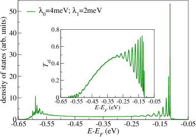
Figure 1: (Color online) Density of states and transmission of Poly-(GC) with 26 base pairs and the following parameters: base pair on-site energy $\epsilon_{G}=-0.35\,e\rm V$, Fermi energy $E_{F}=0\,e\rm V$, vibrational energy $\hbar\omega_{0}=0.01\,e\rm V$, cutoff $\hbar\omega_{c}=0.03\,e\rm V$, linewidth $\Gamma=0.1\,e\rm V$ and room temperature $k_{B}T=0.025\,e\rm V$. The strong asymmetry of the curves with respect to the band center is a consequence of the non-local electron-vibron coupling $\lambda_{1}$.

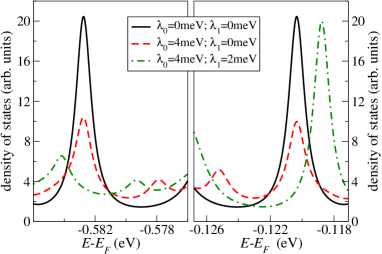
Figure 2: (Color online) Density of states of Poly-(GC) with 26 base pairs and parameters as in Fig. 1. The solid line shows the purely electronic resonances. Inclusion of only a local electron-vibron coupling $\lambda_{0}$ reduces the weight at the original electronic resonance in favor of ‘vibron satellites’ (dashed line). The addition of a non-local electron-vibron coupling $\lambda_{1}$ (dash-dotted line) introduces shifts of the resonance peaks to the ‘outside’ (changing the effective band width) as well as a strong asymmetry in the height of the resonances.

To further elucidate this connection we take a closer look at the upper and lower band edge of the density of states (see Fig. 2). Without electron-vibron coupling (solid curve) we see the electronic resonances of equal height, positioned at the energies corresponding to the ‘Bloch’-like states of this finite size tight-binding chain. If we include only local electron-vibron coupling (dashed line), vibron satellite states appear, and the spectral weight of the original electronic resonances decreases, consistent with the spectral sum rule. Note that the displayed vibron satellites are not satellites of the displayed electronic states, but emerge from other states at higher and lower energies. Indeed the difference in peak positions is not equal to $\hbar\omega_{0}$. Inclusion of the non-local coupling $\lambda_{1}$ shifts the original electronic resonance positions (dashed-dotted line). In the present example, with positive sign of $\lambda_{1}$, the resonances are shifted to the ‘outside’, corresponding to an effective increase in bandwidth; for the opposite sign of $\lambda_{1}$ the resonances shift to the ‘inside’. Furthermore, a distinct asymmetry of the resonances is observed, i.e. the upper band edge states have a larger peak height than the lower band edge states. This asymmetry in the density of states comes with a corresponding asymmetry in the elastic transmission, see Fig. 1 for the overall view.

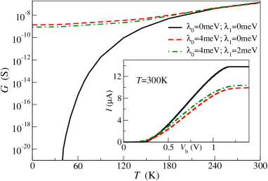
Figure 3: (Color online) Zero-bias conductance and $I$-$V$-characteristics for Poly-(GC) with 26 base pairs and parameters as in Fig. 1. The inclusion of vibrons increases the zero-bias conductance at low temperatures ($k_{\rm B}T$ roughly below $\hbar\omega_{0}$) by several orders of magnitude. At room temperature, however, the zero bias conductance is slightly reduced. Inset: the $I$-$V$-characteristics shows a ‘semiconducting’ behavior at room temperature. The non-local electron-vibron coupling $\lambda_{1}$ increases both the non-linear conductance in the gap and around the threshold, leading to a slightly enhanced current.

As shown in Fig. 3 the coupling to vibrons strongly increases the zero-bias conductance at low temperatures, whereas at high temperatures the conductance slightly decreases (dashed and dash-dotted line). This effect has been observed before, e.g. in Ref. Gutierrez et al., 2005. At low temperatures, the conductance is increased since the density of states at the Fermi energy is effectively enhanced due to (broadened) vibronic ‘satellite’ resonances. The transport remains ‘elastic’, i.e. electrons enter and leave the DNA at the same energy (first contribution to the current Eq. 14). At sufficiently high temperatures, however, the back scattering of electrons due to vibrons reduces the conductance in comparison to situation without electron-vibron coupling (solid line).

The inset of Fig. 3 shows a typical $I$-$V$-characteristic for the system. A quasi-semiconducting behavior is observed, where the size of the conductance gap is determined by the energetic distance of the Fermi energy to the (closest) band edge. After crossing this threshold, the current increases roughly linear with the voltage until at larger bias it saturates when the right chemical potential drops below the lower transmission band edge. Small step-like wiggles due to the ‘discrete’ electronic states are visible at low temperature (not shown), but are smeared out at room temperature. The current is dominated by the elastic transmission, as expected for a homogeneous system.

The non-local coupling has a quantitative effect on the nature of the $I$-$V$-curve. The zero bias conductance as well as the non-linear conductance around the threshold are increased by close to a factor $1.2$. This increase is directly related to the enhancement of the density of states and elastic transmission around the upper band edge (see Figs. 1 and 2).

III.2 Inhomogeneous DNA

Inhomogeneous DNA sequences show a transport behavior which differs significantly from that of the homogeneous Poly-(GC) sequence. As a specific example, we analyze the sequence 5’-CAT TAA TGC TAT GCA GAA AAT CTT AG-3’ (plus complementary strand), which has been investigated experimentally by Porath et al.Cohen et al. (2005).

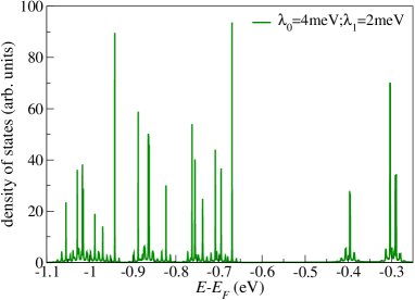
Figure 4: (Color online) Density of states of an inhomogeneous DNA with sequence (5’-CAT TAA TGC TAT GCA GAA AAT CTT AG-3’). We chose the following parameters: GC on-site energy $\epsilon_{G}=-0.35\,e\rm V$, AT on-site energy $\epsilon_{A}=-0.86\,e\rm V$ , Fermi energy $E_{F}=0\,e\rm V$, vibron energy $\hbar\omega_{0}=0.01\,e\rm V$, cutoff $\hbar\omega_{c}=0.03\,e\rm V$, linewidth $\Gamma=0.1\,e\rm V$ and room temperature $k_{B}T=0.025\,e\rm V$. The density of states is fragmented into ‘bunches’ of strongly localized states with very low elastic transmission.

The density of states is displayed in Fig. 4. Rather than traces of bands it now shows discrete ‘bunches’ of states due to the disorder in the sequence. All states are strongly localized, extending over at most a few base pairs Klotsa et al. (2005). The right-most (largest energy) bunch of states is due to the GC base pairs. Two of these GC pairs are the only base pairs that are directly coupled to the metallic electrodes. Note that the equilibrium Fermi level is set at $E_{F}=0\,e\rm V$, roughly $0.35\,e\rm V$ above these states. The first states with mostly AT character are located around $-0.7\,e\rm V$.

As to be expected the elastic transmission through these localized states is extremely low. The largest contribution to the elastic transmission stems from the AT-like states around an energy $\epsilon_{A}=-0.86\,e\rm V$ (note that the considered sequence is AT rich). But even these states have an elastic transmission of less than $10^{-14}$ for the parameters we use. Consequently, the ‘elastic’ quasi-ballistic transmission of electrons is completely negligible for the considered sequence.

In spite of the localization of the electron states, a rather significant current can be transmitted, as displayed in Fig. 5. It is due to the inelastic contributions to transport, where electrons dissipate (or absorb) energy during their motion through the DNA. Roughly speaking, the transported electrons excite the vibrons which in turn either dissipate their energy to the environment or ‘promote’ other electrons, thus increasing their probability to hop to neighboring but energetically distant base pairs. This inelastic transmission strongly depends on the specific states (in contrast to the band-like transmission for the homogeneous sequence). As a consequence, the inelastic transmission of different states can differ by several orders of magnitude. Together with the bunched density of states this leads to the step-like behavior for the current displayed in Fig. 5. The first step centered around $V_{b}\sim 0.7\,\rm V$ roughly corresponds to states with GC character, whereas the second step corresponds to states with mixed AT-GC character at $-0.7\,e\rm V$. Here, the GC states display a larger inelastic transmission as can be seen from the large non-linear conductance peak around $V_{b}\sim 0.6-0.7\,\rm V$ (see inset of Fig. 5).

The non-local electron-vibron coupling $\lambda_{1}$ for this sequence leads to qualitative change of the $I$-$V$-characteristics, depending on the details of the nature of the states and therefore explicitly on the DNA sequence. The current on the lowest bias plateau is increased relative to the case with only local electron-vibron coupling, although the GC states do barely shift towards the Fermi energy. However, the inelastic transmission of the states is slightly increased (see inset), leading to an increased current on the first plateau (dashed line).

In contrast, the conductance due to states with mixed AT-GC nature is much reduced (almost by a factor of two, see middle peak in the inset of Fig. 5) which leads to a smaller increase of the current for the middle step. Obviously, the transmission of these mixed states is reduced by the ‘vibron assisted electron hopping’. On the other hand, the last step at $\sim 2V$ is almost unaffected.

While the changes of the $I$-$V$-characteristics due to non-local electron-vibron coupling are relatively small for the present sequence and model parameters, the observed sensitivity of the inelastic transmission suggests that other sequences could display much larger effects. Furthermore, quantum chemistry calculations Starikov (2005) suggest that the local and non-local electron-vibron couplings can be of the order of $\sim 10\,\mathrm{m}e\rm V$, i.e. larger than what we considered here. Inhomogeneities in the electron-vibron coupling, not covered in the present calculation, might have a further impact.

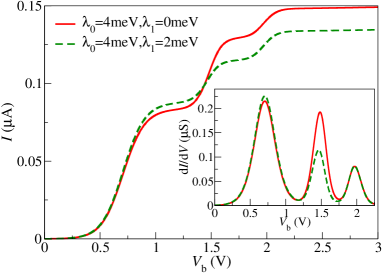
Figure 5: (Color online) $I$-$V$-characteristics and differential conductance for an inhomogeneous DNA with sequence (5’-CAT TAA TGC TAT GCA GAA AAT CTT AG-3’). Parameters are the same as in Fig. 4. The inclusion of a non-local electron-vibron coupling $\lambda_{1}$ leads to changes in the conductance, depending on the nature of the relevant state.

The DNA sequence we considered was investigated in transport experiments, and we should compare the experimental and theoretical results. As some important factors are still not well determined, a quantitative comparison is not feasible. However, we observe both in experiment and theory roughly a ‘semiconducting’ $I$-$V$-characteristics with (sometimes) steplike features. The size of the currents is roughly comparable, of the order of $\sim 80\,\mathrm{nA}$ at a bias of $V_{b}=1\,\mathrm{V}$. As the choice of the position of the Fermi energy defines the size of the ‘semiconducting’ gap, this gap could be adjusted to fit the experiment. On the other hand, the value of the current for this sequence (with parameters derived from quantum chemistry calculations) can not be simply scaled by changing a single ‘free’ parameter like the electrode-DNA coupling $\Gamma$.

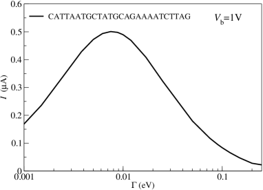
Figure 6: Current at a bias of $V_{b}=1\,\mathrm{V}$ as a function of electrode-DNA coupling $\Gamma$ for the inhomogeneous DNA with sequence (5’-CAT TAA TGC TAT GCA GAA AAT CTT AG-3’). Other parameters are the same as in Fig. 4. The current is a non-monotonous function of $\Gamma$ and peaks around a value $\Gamma_{max}$ where the imaginary part of the vibron self energy $\Sigma_{\rm vib}$ is of the same size as $\Gamma$.

For the case of the homogeneous sequence, the current at a given bias (say, at $V_{b}=1\,\mathrm{V}$) grows monotonically with increasing $\Gamma$ (as long $\Gamma$ is smaller than the hopping amplitude $t_{ij}$), as is expected from quasi-ballistic Landauer-type transport. In contrast, for the inhomogeneous sequence, the current is a non-monotonic function of $\Gamma$, see Fig. 6. In particular, the current at the first plateau (at $V_{b}=1\,\mathrm{V}$) initially grows as we decrease $\Gamma$ from the value used in the above figures ($\Gamma=0.1\,e\mathrm{V}$), up to a point at which the imaginary part of the vibron self energy $\Sigma_{\rm vib}$ is of the same size as $\Gamma$. This happens around $\Gamma_{max}\sim 0.01\,e\mathrm{V}$. The current at $\Gamma_{max}$ is of order of $\sim 500\,\mathrm{nA}$. If $\Gamma$ is decreased further, the current drops rapidly from the maximal value. On the other hand, if $\Gamma$ is increased above the value $\Gamma=0.1\,e\mathrm{V}$, the current also drops initially, before at very large $\Gamma$ quasi-ballistic transport becomes dominant and the current increases again (not shown in the figure).

Summarizing these results, we conclude that for the given model parameters, i.e. for values of $\Gamma$ in the large range $1-200\,\mathrm{m}e\rm V$, likely to be realistic for present-days transport experiments in DNA, the current at the first plateau lies in the range of $50-500\,\mathrm{nA}$.

IV Summary

To summarize, we have presented a technique that allows the computation of electron transport through short sequences of DNA, including local and non-local coupling to vibrations and a dissipative environment. Using an equation-of-motion approach we identify elastic and inelastic contributions to the current. For homogeneous DNA sequences, the transport is dominated by elastic quasi-ballistic contributions through a band-like density of states (Fig. 1,2), which display an asymmetry due to the non-local electron-vibron coupling. The coupling to vibrations strongly enhances the zero-bias conductance at low temperatures. The current at finite bias above the ‘semiconducting’ gap, however, is only quantitatively modified by the non-local electron-vibron coupling (Fig. 3). For inhomogeneous DNA sequences, the transport is almost entirely due to inelastic processes, the effectiveness of which is strongly sequence dependent (Fig. 4). For the considered example sequence the non-local electron-vibron coupling qualitatively modifies the $I$-$V$-characteristics (Fig. 5). We also point out that the current through inhomogeneous DNA sequences depends non-monotonically on the electrode-DNA coupling $\Gamma$ (Fig. 6).

Acknowledgments. We acknowledge stimulating discussions with J. Viljas, J. Starikov, A.-P. Jauho, E. Scheer and W. Wenzel. We also thank the Landesstiftung Baden-Württemberg for financial support via the Kompetenznetz “Funktionelle Nanostrukturen”.

Appendix A Equation of motion

Before applying the equation of motion we separate the retarded electron Green function into two parts,

$$G_{kl}^{\mathrm{ret}}(t) = -i\theta(t)\left\langle\left\{a_{k}(t)\chi(t),a_{l}^{\dagger}\chi^{\dagger}\right\}\right\rangle$$ (17)

$$= \underbrace{-i\theta(t)\left\langle a_{k}(t)\chi(t)a_{l}^{\dagger}\chi^{\dagger}\right\rangle}_{G_{kl}^{(1)}(t)}$$

$$\underbrace{-i\theta(t)\left\langle a_{l}^{\dagger}\chi^{\dagger}a_{k}(t)\chi(t)\right\rangle}_{G_{kl}^{(2)}(t)}\,.$$

This is necessary, because for $G_{kl}^{(1)}(t)$ and $G_{kl}^{(2)}(t)$ self-consistency equations can be derived via the equation-of-motion technique (EOM) (The equation of motion applied to the retarded Green function $G_{kl}^{\mathrm{ret}}(t)$ leads to an equation containing not only the retarded Green function). The EOM technique for an interacting system generates a hierarchy of correlation functions that does not close in itself. Therefore, an appropriate truncation scheme needs to be applied. Here we close the hierarchy at the first possible level, i.e. we neglect all higher order Green functions beyond the one defined above.

From the equation of motion we obtain the following expression for $G_{kl}^{(1)}(t)$ defined in Eq. (17)

$$\sum_{j}\left[(i\frac{\partial}{\partial t}-\epsilon_{k})\delta_{jk}+t_{kj}\right]\,G_{jl}^{(1)}(t)$$

$$=\delta(t)\left\langle a_{k}a_{l}^{\dagger}\right\rangle+i\theta(t)\Delta\left\langle a_{k}(t)\chi(t)a_{l}^{\dagger}\chi^{\dagger}\right\rangle$$

$$-i\theta(t)\left\{\sum_{j\neq k,\alpha}\lambda_{kj}\,\left\langle a_{j}(t)\left[B_{\alpha}(t)+B_{\alpha}^{\dagger}(t)\right]\chi(t)a_{l}^{\dagger}\chi^{\dagger}\right\rangle\right.$$

$$+\sum_{\alpha}\lambda_{0}\,\left\langle a_{k}(t)B_{\alpha}(t)\chi(t)a_{l}^{\dagger}\chi^{\dagger}\right\rangle$$

$$+\sum_{\alpha}\sum_{i,j;j\neq i}\frac{2\,\lambda_{ij}\,\lambda_{0}}{\omega_{\alpha}}\left\langle a_{k}(t)a_{i}^{\dagger}(t)a_{j}(t)\chi(t)a_{l}^{\dagger}\chi^{\dagger}\right\rangle$$

$$+\sum_{\alpha}\lambda_{0}\,\left\langle a_{k}(t)\chi(t)B_{\alpha}^{\dagger}(t)a_{l}^{\dagger}\chi^{\dagger}\right\rangle+\left.\sum_{n}V_{nk}^{*}\left\langle c_{n}(t)a_{l}^{\dagger}\chi_{l}^{\dagger}\right\rangle\right\}$$ (18)

and a similar relation for $G_{kl}^{(2)}(t)$.

The expressions $\left\langle a_{j}(t)B_{\alpha}(t)\chi(t)a_{l}^{\dagger}\chi^{\dagger}\right\rangle$ and similar higher order correlation function are approximated by assuming

$$\left\langle a_{j}(t)B_{\alpha}(t)\chi(t)a_{l}^{\dagger}\chi^{\dagger}\right\rangle_{\bar{H}}\approx F_{\alpha}(t)\left\langle a_{j}(t)\chi(t)a_{l}^{\dagger}\chi^{\dagger}\right\rangle_{\bar{H}}.$$ (19)

The function $F_{\alpha}(t)$ is obtained by considering a Hamiltonian $H_{0}$ without electron-vibron coupling and calculating the same higher order correlation function $\left\langle a_{j}(t)B_{\alpha}(t)\chi(t)a_{l}^{\dagger}\chi^{\dagger}\right\rangle_{H_{0}}$, where now the average is taken with respect to $H_{0}$. Then the electronic and vibronic correlators factorize,

$$\left\langle a_{j}(t)B_{\alpha}(t)\chi(t)a_{l}^{\dagger}\chi^{\dagger}\right\rangle_{H_{0}}=\left\langle a_{j}(t)a_{l}^{\dagger}\right\rangle_{H_{0}^{\rm el}}\left\langle B_{\alpha}(t)\chi(t)\chi^{\dagger}\right\rangle_{H_{0}^{\rm vib}}\,,$$ (20)

where $H_{0}^{\rm el}$ and $H_{0}^{\rm vib}$ are the electronic and vibronic parts of $H_{0}$.

After some straight-forward algebra (cf Ref. Boettger and Bryksin, 1985) we obtain

$$\left\langle B_{\alpha}(t)\chi(t)\chi^{\dagger}\right\rangle_{H_{0}^{\rm vib}}=F_{\alpha}(t)\left\langle\chi(t)\chi^{\dagger}\right\rangle_{H_{0}^{\rm vib}}$$ (21)

and consequently

$$\left\langle a_{j}(t)B_{\alpha}(t)\chi(t)a_{l}^{\dagger}\chi^{\dagger}\right\rangle_{H_{0}}=F_{\alpha}(t)\left\langle a_{j}(t)\chi(t)a_{l}^{\dagger}\chi^{\dagger}\right\rangle_{H_{0}}\,.$$ (22)

Because the strength of the electron-vibron coupling in $\bar{H}$ is proportional to $\lambda_{1}$, this approximation is valid for not too large values of $\lambda_{1}$.

Expressions like $\left\langle a_{l}^{\dagger}\chi^{\dagger}a_{k}(t)a_{i}^{\dagger}(t)a_{j}(t)\chi(t)\right\rangle$ are treated in a mean-field like manner:

$$\left\langle a_{k}(t)a_{i}^{\dagger}(t)a_{j}(t)\chi(t)a_{l}^{\dagger}\chi^{\dagger}\right\rangle$$ (23)

$$\approx \left\langle a_{k}(t)a_{i}^{\dagger}(t)\right\rangle\left\langle a_{j}(t)\chi(t)a_{l}^{\dagger}\chi^{\dagger}\right\rangle$$

$$- \left\langle a_{j}(t)a_{i}^{\dagger}(t)\right\rangle\left\langle a_{k}(t)\chi(t)a_{l}^{\dagger}\chi^{\dagger}\right\rangle\,.$$

Using the above approximations we obtain after Fourier transformation and crossover to the continuous sprectrum

$$\sum_{j}\left[(E-\epsilon_{k})\delta_{jk}+t_{kj}\right]\,G_{jl}^{(1)}(E)$$ (24)

$$=\left\langle a_{k}a_{l}^{\dagger}\right\rangle-\Delta G_{kl}^{(1)}(E)$$

$$+\int d\omega D(\omega)\Bigg{\{}-\sum_{i}\sum_{j\neq i}\left\langle a_{j}a_{i}^{\dagger}\right\rangle\frac{2\lambda_{ij}\lambda_{0}}{\omega}G_{kl}^{(1)}(E)$$

$$+\sum_{i}\sum_{j\neq i}\left\langle a_{k}a_{i}^{\dagger}\right\rangle\frac{2\lambda_{ij}\lambda_{0}}{\omega}G_{jl}^{(1)}(E)$$

$$+\sum_{j\neq k}\frac{\lambda_{kj}\lambda_{0}}{\omega}\left[\int dte^{iEt}\left[F_{1}(t,\omega)-1\right]\,G_{jl}^{(1)}(t)\right]$$

$$+\frac{\lambda_{0}^{2}}{\omega}\left[\int dte^{iEt}F_{1}(t,\omega)\,G_{kl}^{(1)}(t)\right]\Bigg{\}}$$

$$+\sum_{j}\Sigma_{kj}^{\rm L}G_{jl}^{(1)}(E)+\sum_{j}\Sigma_{kj}^{\rm R}G_{jl}^{(1)}(E)$$

with

$$F_{1}(t,\omega) = \left(N(\omega)+1\right)e^{-i\omega t}-N(\omega)e^{i\omega t}\,,$$ (25)

and $\Sigma_{\rm R/L}$ are the right and left electrode self-energies. A similar relation holds for $G_{kl}^{(2)}(E)$.

We can now identify

$$(E-\epsilon_{k})\delta_{jk}+t_{jk}+i0^{+}=\left[G_{0}^{\mathrm{ret}}(E)\right]_{jk}^{-1}\,,$$ (26)

where $G_{0}^{\rm ret}(E)$ is the retarded Green function for the isolated DNA without electron-vibron interaction. The validity of this equation can easily be seen by computing the equation of motion for $G^{\mathrm{ret}}(t)$ for the isolated DNA without electron-vibron coupling.

References

- Braun et al. (1998) E. Braun, Y. Eichen, U. Sivan, and G. Ben-Yoseph, Nature 391, 775 (1998).
- Porath et al. (2000) D. Porath, A. Bezryadin, S. de Vries, and C. Dekker, Nature 403, 635 (2000).
- Xu et al. (2004) B. Q. Xu, P. M. Zhang, X. L. Li, and N. J. Tao, Nano Lett. 4, 1105 (2004).
- Starikov (2005) E. B. Starikov, Phil. Mag. 85, 3435 (2005).
- Asai (2004) Y. Asai, Phys. Rev. Lett. 93, 246102 (2004).
- Galperin et al. (2006) M. Galperin, A. Nitzan, and M. A. Ratner, Phys. Rev. B 73, 045314 (2006).
- Gutierrez et al. (2005) R. Gutierrez, S. Mandal, and G. Cuniberti, Phys. Rev. B 71, 235116 (2005).
- (8) R. Gutierrez, S. Mohapatra, H. Cohen, D. Porath, and G. Cuniberti, Phys. Rev. B 74, 235105 (2006).
- Voityuk et al. (2000) A. A. Voityuk, J. Jortner, M. Bixon, and N. Rösch, Chem. Phys. Lett. 324, 430 (2000).
- Senthilkumar et al. (2005) K. Senthilkumar, F. C. Grozema, C. F. Guerra, F. M. Bickelhaupt, F. D. Lewis, Y. A. Berlin, M. A. Ratner, and L. D. A. Siebbeles, J. Am. Chem. Soc. 127, 14894 (2005).
- Conwell and Rakhmanova (2000) E. M. Conwell and S. V. Rakhmanova, Proc. Natl. Acad. Sci. USA 97, 4556 (2000).
- Henderson et al. (1999) P. T. Henderson, D. Jones, G. Hampikian, Y. Kan, and G. B. Schuster, Proc. Natl. Acad. Sci. USA 96, 8353 (1999).
- Yoo et al. (2001) K. H. Yoo, D. H. Ha, J. O. Lee, J. W. Park, J. Kim, J. J. Kim, H. Y. Lee, T. Kawai, and H. Y. Choi, Phys. Rev. Lett. 87, 198102 (2001).
- Troisi and Orlandi (2002) A. Troisi and G. Orlandi, J. Phys. Chem. B 106 (2002).
- Artacho et al. (2003) E. Artacho, M. Machado, D. Sanchez-Portal, P. Ordejon, and J. M. Soler, Mol. Phys. 101, 1587 (2003).
- Lewis et al. (2003) J. P. Lewis, T. E. Cheatham, E. B. Starikov, H. Wang, and O. F. Sankey, J. Phys. Chem. B 107, 2581 (2003).
- Endres et al. (2004) R. G. Endres, D. L. Cox, and R. R. P. Songh, Rev. Mod. Phys. 76, 195 (2004).
- Mahan (2000) G. D. Mahan, Many-Particle Physics (Kluwer Academic/Plenum Publishers, 2000).
- Boettger and Bryksin (1985) H. Boettger and V. Bryksin, Hopping conduction in Solids (Akademie Verlag Berlin, 1985).
- Weiss (1999) U. Weiss, Quantum Dissipative Systems (World Scientific, 1999).
- Meir and Wingreen (1992) Y. Meir and N. S. Wingreen, Phys. Rev. Lett. 68, 2512 (1992).
- Galperin et al. (2004) M. Galperin, M. A. Ratner, and A. Nitzan, J. Chem. Phys. 121 (2004).
- Viljas et al. (2005) J. K. Viljas, J. C. Cuevas, F. Pauly, and M. Häfner, Phys. Rev. B 72, 245415 (2005).
- Cohen et al. (2005) H. Cohen, C. Nogues, R. Naaman, and D. Porath, Proc. Natl. Acad. Sci. USA 102, 11589 (2005).
- Klotsa et al. (2005) D. Klotsa, R. A. Römer, and M. S. Turner, Biophys. J. 89, 2187 (2005).