Collective behavior of interacting self-propelled particles

Abstract

We discuss biologically inspired, inherently non-equilibrium self-propelled particle models, in which the particles interact with their neighbours by choosing at each time step the local average direction of motion. We summarize some of the results of large scale simulations and theoretical approaches to the problem.

1 Introduction

The collective motion of various organisms like the flocking of birds, swimming of schools of fish, motion of herds of quadrupeds (see, e.g. [1, 2] and references therein) migrating bacteria [3], molds [4], ants [5] or pedestrians [6] is a fascinating phenomenon of nature. We address the question whether there are some global, perhaps universal features of this type of behavior when many organisms are involved and parameters like the level of perturbations or the mean distance between the individuals are changed.

These studies are also motivated by recent developments in areas related to statistical physics. Concepts originated from the physics of phase transitions in equilibrium systems [7] such as scale invariance and renormalization have also been shown to be useful in the understanding of various non-equilibrium systems, typical in our natural and social environment. Motion and related transport phenomena represent further characteristic aspects of many non-equilibrium processes and they are essential features of most living systems.

To study the collective motion of large groups of organisms, the concept of self propelled particle (SPP) models was introduced in [8]. As the motion of flocking organisms is usually controlled by interactions with their neighbors [1], the SPP models consist of locally interacting particles with an intrinsic driving force, hence with a finite steady velocity. Because of their simplicity, such models represent a statistical approach complementing other studies which take into account more details of the actual behavior [6, 9, 10], but treat only a moderate number of organisms and concentrate less on the large scale behavior.

In spite of the analogies with ferromagnetic models, the general behavior of SPP systems can be quite different from those observed in equilibrium magnets. In particular, equilibrium ferromagnets possessing continuous rotational symmetry do not have ordered phase at finite temperatures in two dimensions [11]. However, in 2d SPP models an ordered phase can exist at finite noise levels (temperatures) as it was first demonstrated by simulations [8, 12] and explained by a theory of flocking developed by Toner and Tu [13, 14]. Further studies revealed that modeling collective motion leads to interesting specific results in all of the relevant dimensions (from 1 to 3) [15, 16].

2 Discrete models

The 2d system.

The simplest model, introduced in [8], consists of particles moving on a plane with periodic boundary condition. The particles are characterized by their (off-lattice) location $\vec{x}_{i}$ and velocity $\vec{v}_{i}$ pointing in direction $\vartheta_{i}$. The self-propelled nature of the particles is manifested by keeping the magnitude of the velocity fixed to $v_{0}$. Particles interact through the following local rule: at each time step a given particle assumes the average direction of motion of the particles in its local neighborhood $S(i)$ (e.g., in a circle of some given radius centered at the position of the $i$th particle) with some uncertainty, as described by

$$\vartheta_{i}(t+\Delta t)=\langle\vartheta(t)\rangle_{S(i)}+\xi,$$ (1)

where the noise $\xi$ is a random variable with a uniform distribution in the interval $[-\eta/2,\eta/2]$. The locations of the particles are updated as

$$\vec{x}_{i}(t+\Delta t)=\vec{x}_{i}(t)+\vec{v}_{i}(t)\Delta t$$ (2)

with $|\vec{v}_{i}|=v_{0}=const$.

The model defined by Eqs. (1) and (2) is a transport related, non-equilibrium analog of ferromagnetic models [17]. The analogy is as follows: the Hamiltonian tending to align the spins in the same direction in the case of equilibrium ferromagnets is replaced by the rule of aligning the direction of motion of particles, and the amplitude of the random perturbations can be considered proportional to the temperature for $\eta\ll 1$. From a hydrodynamical point of view, in SPP systems the momentum of the particles is not conserved and – as was pointed out in [18] – the Galilean invariance is broken. Thus, the flow fields emerging in these models can considerably differ from the usual behavior of fluids.

Critical exponents.

The model defined through Eqs. (1) and (2) with circular interaction range was studied by performing large-scale simulations. Due to the simplicity of the model, only two control parameters should be distinguished: the (average) density of particles $\varrho=N/L^{2}$ (where $N$ is the number of particles and $L$ is the system size in units of the interaction range) and the amplitude of the noise $\eta$. Depending on the value of these parameters the model can exhibit various type of behaviors as Fig. 1 demonstrates.

Figure 1: Typical configurations of the positions of SPPs displayed for various values of density and noise. For small enough noise coherently moving clusters can be identified in the system, which gradually disappear as the noise amplitude is increased. The noise amplitudes applied in the simulations were the following: $\eta=0.2$ (a,d); $\eta=0.4$ (b,e); $\eta=0.8$ (c,f); $\eta=0.6$ (g); $\eta=1.2$ (h) and $\eta=1.8$ (i). The corresponding order parameter values are: $\phi=0.75$ (a,d); $\phi=0.19$ (b); $\phi=0.025$ (c); $\phi=0.3$ (e,h); $\phi=0.05$ (f,i) and $\phi=0.85$ (g). The scales are given in units of the interaction length.

For the statistical characterization of the system a well-suited order parameter is the magnitude of the average momentum of the particles: $\phi\equiv{1\over N}\left|\sum_{j}\vec{v}_{j}\right|.$ This measure of the net flow is non-zero in the ordered phase, and vanishes (for an infinite system) in the disordered phase. Since the simulations were started from a random, disordered configuration, $\phi(t=0)\approx 0$. After some relaxation time a steady state emerges indicated by the convergence of the cumulative average $(1/\tau)\int^{\tau}_{0}\phi(t)dt$. The stationary values of $\phi$ are plotted in Fig. 2 vs $\eta$ for various parameters. For weak noise the model displays an ordered motion, i.e. $\phi\approx 1$, which disappears in a continuous manner by increasing $\eta$. As $L\rightarrow\infty$, the numerical results show the presence of a phase transition described by

$$\phi(\eta)\sim\cases{\Bigl{(}{\eta_{c}(\varrho)-\eta\over\eta_{c}(\varrho)}\Bigr{)}^{\beta}&for $\eta<\eta_{c}(\varrho)$\cr 0&for $\eta>\eta_{c}(\varrho)$\cr},$$ (3)

where $\eta_{c}(\varrho)$ is the critical noise amplitude that separates the ordered and disordered phases and $\beta_{2d}=0.42\pm 0.03$, was found [12] to be different from the the mean-field value $1/2$. This large-scale behavior does not depend on the specific choice of the microscopic details as Fig. 2 demonstrates.

     

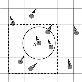
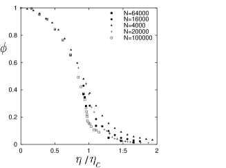
Figure 2: Left: Schematic illustration of the various realizations of the SPP model. Particles move off-lattice on a plane and interact with other particles located in the surrounding, which can be either a circle ($S_{1}$) or 9 neighboring cells in an underlying lattice ($S_{2}$). We plot these interaction areas for particle $A$ with a solid and dashed line, respectively. Right: The average momentum of the system in the steady state vs the rescaled noise amplitude $\eta/\eta_{c}$ for various interaction ranges, densities and system sizes. Open symbols refer to interaction type $S_{1}$ and $\varrho=1$ while filled symbols refer to interaction type $S_{2}$ and $\varrho=2$. The order present at small $\eta$ disappears in a continuous manner reminiscent of second order phase transitions for $N\rightarrow\infty$.

As a further analogy with equilibrium phase transitions, the fluctuations of the order parameter also increase on approaching the critical line [12]. The tails of the curves are symmetric, and decay as power-laws with an exponent $\gamma$ close to $2$, which value is, again, different from the mean-field result.

Next we discuss the role of density. The long-range ordered phase is present for any $\varrho$, but for a fixed value of $\eta$, $\phi$ vanishes with decreasing $\varrho$. The critical line $\eta_{c}(\varrho)$ in the $\eta-\varrho$ parameter space was found to follow

$$\eta_{c}(\varrho)\sim\varrho^{\kappa},$$ (4)

with $\kappa=0.45\pm 0.05$ for $\varrho\ll 1$. This critical line is qualitatively different from that of the diluted ferromagnets, since here the critical density at $\eta\rightarrow 0$ (corresponding to the percolation threshold for diluted ferromagnets, see, e.g., [17]) is vanishing.

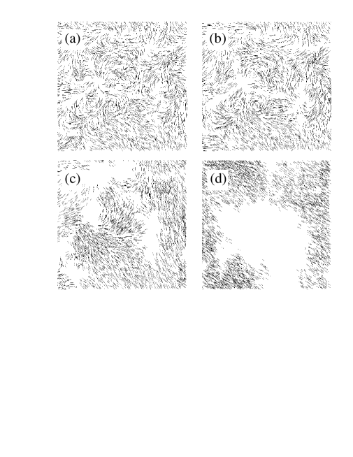
Figure 3: Snapshots of the time development of a system with $N=4000$, $L=40$ and $v_{0}=0.01$ at $50$ (a), $100$ (b), $400$ (c) and $3000$ (d) steps. First the behavior is reminiscent of the equilibrium $XY$ model, where the long range order is missing since vortices are present in the system. Here the vortices are unstable, and finally a self-organized long-range order develops. (After [12].)

These findings indicate that SPP systems can be quite well characterized using the framework of classical critical phenomena, but also show surprising features when compared to the analogous equilibrium systems. The velocity $v_{0}$ provides a control parameter which switches between the SPP behavior ($v_{0}>0$) and an $XY$ ferromagnet ($v_{0}=0$). Indeed, for $v_{0}=0$ Kosterlitz-Thouless vortices [19] can be observed in the system, which are unstable (Fig. 3.) for any nonzero $v_{0}$ investigated in [12].

Correlation functions.

Beside the calculation of the order parameter, it is insightful to characterize the configurations with correlation functions, such as the velocity-velocity correlation function

$$C(\vec{r})=\left\langle\vec{v}(\vec{r}+\vec{r}^{\prime},t)\vec{v}(\vec{r}^{\prime},t)\right\rangle_{\vec{r}^{\prime},t}$$ (5)

where $\vec{v}(\vec{r},t)$ is the coarse-grained velocity field and the average is taken over all possible values of $\vec{r}^{\prime}$ and $t$. The system is ordered on the macroscopic scale if $C_{\infty}=\lim_{|\vec{r}|\rightarrow\infty}C(\vec{r})>0$. The decay of the fluctuations is given by the connected piece of the correlation function $C_{C}(\vec{r})$, defined as $C_{C}(\vec{r})=C(\vec{r})-C_{\infty}$.

One of the major result of the analysis of Toner and Tu [14] was that the attenuation of fluctuations is anisotropic in a SPP flock. In particular, they predicted that within a certain length scale $|\vec{r}|<\ell$, $C(\vec{r})$ decays as

$$C(\vec{r})\sim r_{\perp}^{-2/5}$$ (6)

with $r_{\perp}$ and $r_{||}$ being the orthogonal and parallel projection of $\vec{r}$ relative to the average direction of motion $\left\langle\vec{v}(\vec{r}^{\prime},t)\right\rangle_{\vec{r}^{\prime}}$, respectively.

Figure 4: Equal time velocity-velocity correlation functions characterizing the decay of correlations parallel and perpendicular to the average direction of motion of the flock. $C_{||}$ and $C_{\perp}$ were calculated for systems with circular interaction range, $N=4000$, $L=480$ and $\eta=0.02$ (a), $\eta=0.32$ (b). At these parameter values the critical noise amplitude is at $\eta_{c}\approx 0.2$. The solid line in (a) represents a power-law fit on $C_{C}$ with the predicted exponent $-2/5$.

We calculated the equal-time velocity-velocity correlation function in $(r_{\perp}$, $r_{||})$ base for various time moments and averaged them to obtain $C(\vec{r})$. To demonstrate the predicted anisotropy of the correlation functions, in Fig. 4 curves are plotted which represent averages of points for which either the $r_{\perp}>r_{||}$ or the $r_{\perp}<r_{||}$ relation holds:

$$C_{\perp}(r)=\left\langle C(\vec{r})\right\rangle_{|\vec{r}|=r,r_{\perp}>r_{||}},\hskip 14.22636ptC_{||}(r)=\left\langle C(\vec{r})\right\rangle_{|\vec{r}|=r,r_{\perp}<r_{||}}.$$ (7)

For $\eta<\eta_{c}$ the anisotropy of the correlation functions is clearly seen, while the behavior of $C_{\perp}$ is consistent with the predicted (6). In contrast, for $\eta>\eta_{c}$ the curves vanish for large $r$ and the system is isotropic as expected.

Role of boundary conditions.

Simulations [20, 21, 22] with reflective boundaries and a short range repulsive force (constraining the maximal local density in the system) pointed to the importance of the boundary conditions in SPP models.

Figure 5: A possible stationary state of the model with reflective boundary conditions. (After [22])

In such simulations rotation of the particles develop (see Fig. 5) in the high density, low noise regime. The direction of the rotation is selected by spontaneous symmetry breaking, thus both clockwise and anti-clockwise spinning “vortices” can emerge. This rotating state should be distinguished from the Kosterlitz-Thouless vortices [19], since in our case a single vortex develops irrespective to the system size. In Ref. [22] we give examples of such vortices developing in nature.

One and three dimensional SPP systems.

Since in 1d the particles cannot get around each other, some of the important features of the dynamics present in higher dimensions are lost. On the other hand, motion in 1d implies new interesting aspects (groups of the particles have to be able to change their direction for the opposite in an organized manner) and the algorithms used for higher dimensions should be modified to take into account the specific crowding effects typical for 1d (the particles can slow down before changing direction and dense regions may be built up of momentarily oppositely moving particles).

In a way the system studied below can be considered as a model of people, moving in a narrow channel. Imagine that a fire alarm goes on, the tunnel is dark, smoky, everyone is extremely excited. People are both trying to follow the others (to escape together) and behave in an erratic manner (due to smoke and excitement).

Thus, in [15] $N$ off-lattice particles along a line of length $L$ have been considered. The particles are characterized by their coordinate $x_{i}$ and dimensionless velocity $u_{i}$ updated as

$$x_{i}(t+\Delta t)=x_{i}(t)+v_{0}u_{i}(t)\Delta t,$$ (8)

$$u_{i}(t+\Delta t)=G\Bigl{(}\langle u(t)\rangle_{S(i)}\Bigr{)}+\xi_{i}.$$ (9)

The local average velocity $\langle u\rangle_{S(i)}$ for the $i$th particle is calculated over the particles located in the interval $[x_{i}-\Delta,x_{i}+\Delta]$, where $\Delta=1/2$. The function $G$ incorporates both the “propulsion” and “friction” forces which set the velocity to a prescribed value $v_{0}$ on the average: $G(u)>u$ for $u<1$ and $G(u)<u$ for $u>1$. In the numerical simulations [15] one of the simplest choices for $G$ was implemented as

$$G(u)=\cases{(u+1)/2&for $u>0$\cr(u-1)/2&for $u<0$,\cr}$$ (10)

and random initial and periodic boundary conditions were applied.

Again, the emergence of the ordered phase was observed through a second order phase transition [15] with $\beta_{1d}=0.60\pm 0.05$, which is different from both the the mean-field value $1/2$ and $\beta_{2d}\approx 0.4$ found in 2d. The critical line on the $\rho-\eta$ phase diagram also follows (4) with $\kappa_{1d}\approx 1/4$.

In two dimensions an effective long range interaction can build up because the migrating particles have a considerably higher chance to get close to each other and interact than in three dimensions (where, as is well known, random trajectories do not overlap). The less interaction acts against ordering. On the other hand, in three dimensions even regular ferromagnets order. Thus, it is interesting to see how these two competing features change the behavior of 3d SPP systems. The convenient generalization of (1) for the 3d case can be the following [16]:

$$\vec{v}_{i}(t+\Delta t)=v_{0}\hbox{ \bf N}(\hbox{ \bf N}(\langle\vec{v}(t)\rangle_{S(i)})+\vec{\xi}),$$ (11)

where $\hbox{ \bf N}(\vec{u})=\vec{u}/|\vec{u}|$ and the noise $\vec{\xi}$ is uniformly distributed in a sphere of radius $\eta$.

Generally, the behavior of the system was found [16] to be similar to that of described above. The long-range ordered phase was present for any $\varrho$, but for a fixed value of $\eta$, $\phi$ vanished with decreasing $\varrho$. To compare this behavior to the corresponding diluted ferromagnet, $\phi(\eta,\varrho)$ was determined for $v_{0}=0$, when the model reduces to an equilibrium system of randomly distributed ”spins” with a ferromagnetic-like interaction.Again, a major difference was found between the SPP and the equilibrium models: in the static case the system does not order for densities below a critical value close to 1 which corresponds to the percolation threshold of randomly distributed spheres in 3d.

3 Continuum approaches

The 1d case

Now let us focus on the continuum approaches describing the systems in terms of coarse grained velocity and density fields. As the simplest example, let us first investigate the 1d SPP system described in the previous section. In [15] and [23] the following equations were obtained by the integration of the master equation of the microscopic dynamics:

$$\partial_{t}\rho=-v_{0}\partial_{x}(\rho U)+D\partial_{x}^{2}\rho$$ (12)

and

$$\partial_{t}U=f(U)+\mu^{2}\partial_{x}^{2}U+\alpha{(\partial_{x}U)(\partial_{x}\rho)\over\rho}+\zeta,$$ (13)

with $\rho$ and $U$ being the coarse-grained density and dimensionless velocity fileds, respectively. The coefficients $v_{0}$, $D$, $\mu$ and $\alpha$ are determined by the parameters of the microscopical rules of interaction. The function $f(U)$ is antisymmetric with $f(U)>0$ for $0<U<1$ and $f(U)<0$ for $U>1$. The noise $\zeta$ has a zero mean and its standard deviation is proportional to $\rho^{-1/2}$. The coupling term in (13) with coefficient $\alpha$ is derived from the Tailor expansion of the local average velocity as

$$\langle U\rangle(x)={\int_{x-\Delta}^{x+\Delta}U(x^{\prime})\rho(x^{\prime})dx^{\prime}\over\int_{x-\Delta}^{x+\Delta}\rho(x^{\prime})dx^{\prime}}=U+{\Delta^{2}\over 6}\left[\partial_{x}^{2}U+2{(\partial_{x}U)(\partial_{x}\rho)\over\rho}\right]+...$$ (14)

The nonlinear coupling term $(\partial_{x}U)(\partial_{x}\rho)/\rho$ is specific for such SPP systems: it is responsible for the slowing down (and eventually the ”turning back”) of the particles under the influence of a larger number of particles moving oppositely. When two groups of particles move in the opposite direction, the density locally increases and the velocity decreases at the point they meet. Let us consider a particular case, when particles move from left to right and the velocity is locally decreasing while the density is increasing as $x$ increases (particles are moving towards a “wall” formed between two oppositely moving groups). The term $(\partial_{x}u)$ is less, the term $(\partial_{x}\rho)$ is larger than zero in this case. Together they have a negative sign resulting in the slowing down of the local velocity. This is a consequence of the fact that there are more slower particles (in a given neighborhood) in the forward direction than faster particles coming from behind, so the average action experienced by a particle in the point $x$ slows it down.

For $\alpha=0$ the dynamics of the velocity field $U$ is independent of $\rho$, and Eq. (13) is equivalent to the time dependent Ginsburg-Landau $\Phi^{4}$ model of spin chains, where domains of opposite magnetization develop at finite temperatures. As numerical simulations demonstrate [15, 23], for large enough $\alpha$ and low noise the initial domain structure breaks and the system is organized into a single major group traveling in a spontaneously selected direction. This elimination of the domain structure, i.e., the ordering is strongly connected to the linear instability of the domains [15, 23] for large enough $\alpha$.

Hydrodynamics in two and higher dimensions.

To get an insight into the possible analytical treatment of SPP systems in higher dimensions, the Navier-Stokes equations can be applied for a fluid of SPPs, as described in [24]. The two basic equations governing the dynamics of the noiseless “self-propelled fluid” are the continuity equation

$$\partial_{t}\rho+\nabla(\rho{\vec{v}})=0$$ (15)

and the equation of motion

$$\partial_{t}{\vec{v}}+({\vec{v}}\cdot\nabla){\vec{v}} = {\vec{F}}({\vec{v}})-{1\over\tau_{1}}{\vec{v}}+{1\over\tau_{2}}\left(\langle{\vec{v}}\rangle-v\right)-{1\over\rho^{*}}\nabla p+\nu\nabla^{2}{\vec{v}},$$ (16)

where $\rho^{*}$ is the effective density of the particles, $p$ is the pressure, $\nu$ is the kinematic viscosity, ${\vec{F}}({\vec{v}})$ is the intrinsic driving force of biological origin and $\tau_{1}$, $\tau_{2}$ are time scales associated with velocity relaxation resulting from interaction with the environment and the surrounding SPPs, respectively. Let us now go through the terms of Eq. 16.

The self-propulsion can be taken into account as a constant magnitude force acting in the direction of the velocity of the particles as

$${\vec{F}}={v_{0}\over\tau_{1}}{{{\vec{v}}}\over{|{{\vec{v}}}|}},$$ (17)

where $v_{0}$ is the speed determined by the balance of the propulsion and friction forces, i.e., $v_{0}$ would be the speed of a homogeneous fluid.

Taking Taylor expansion of the expression ${1\over\tau_{2}}\left(\langle{\vec{v}}\rangle-v\right)$ describing local velocity alignment yields

$$\langle{{\vec{v}}}\rangle_{\epsilon}-{\vec{v}} = {\int_{|{\vec{\xi}}|<\epsilon}\hbox{d}{\vec{\xi}}\Bigl{(}{{\vec{v}}}\rho+({\vec{\xi}}\nabla){{\vec{v}}}\rho+{1\over 2}({\vec{\xi}}\nabla)^{2}{{\vec{v}}}\rho+\dots\Bigr{)}\over\int_{|{\vec{\xi}}|<\epsilon}\hbox{d}{\vec{\xi}}\Bigl{(}\rho+({\vec{\xi}}\nabla)\rho+{1\over 2}({\vec{\xi}}\nabla)^{2}\rho+\dots\Bigr{)}}-{\vec{v}}$$ (18)

$$= {\epsilon^{2}\over 6}\Bigl{(}{\nabla^{2}({{\vec{v}}}\rho)\over\rho}-{{\vec{v}}}{\nabla^{2}\rho\over\rho}\Bigr{)}+\dots$$

$$= {\epsilon^{2}\over 6}\Bigl{(}\nabla^{2}{{\vec{v}}}+2(\nabla{{\vec{v}}}){\nabla\rho\over\rho}\Bigr{)}+\dots$$

similarly to the 1d case (14). In the following we will consider cases where the density fluctuations are forced to be small. Hence the velocity-density coupling term in (18) is negligible, which is a major difference compared to the previously studied 1d system. Thus, if the relative density changes are small, the velocity alignment can be incorporated with an effective viscosity coefficient $\nu^{*}$ into the viscous term of (16),

In the simplest cases the pressure can be composed of an effective “hydrostatic” pressure, and an externally applied pressure as

$$p=g^{*}\rho+p_{\rm ext}$$ (19)

where $g^{*}$ is a parameter related to the compressibility of the fluid.

Combining (15), (16), (17) and (19) one gets the following final form for the equations of the SPP flow:

$$\partial_{t}\rho+\nabla(\rho{\vec{v}})=0,$$ (20)

and

$$\partial_{t}{\vec{v}}+({\vec{v}}\cdot\nabla){\vec{v}}={v_{0}\over\tau_{1}}{{{\vec{v}}}\over{|{{\vec{v}}}|}}-{1\over\tau_{1}}{\vec{v}}+\nu^{*}\nabla^{2}{\vec{v}}-{g^{*}}\nabla\rho+-{1\over\rho^{*}}\nabla p_{\rm ext}.$$ (21)

It is useful to introduce the characteristic length $\lambda=\sqrt{\nu^{*}\tau_{1}}$ and characteristic time $T={\lambda\over v_{0}}$ and write (20) and (21) in a dimensionless form of

$$\partial_{t^{\prime}}\rho+\nabla^{\prime}(\rho{\vec{v}}^{\prime})=0,$$ (22)

$${\tau_{1}\over T}\left(\partial_{t^{\prime}}{\vec{v}}^{\prime}+({\vec{v}}^{\prime}\cdot\nabla^{\prime}){\vec{v}}^{\prime}\right)={{\vec{v}}^{\prime}\over{|{\vec{v}}^{\prime}|}}-\vec{v}^{\prime}+\nabla^{\prime 2}\vec{v}^{\prime}-g^{\prime}_{1}\nabla^{\prime}\rho+g^{\prime}_{2}\nabla^{\prime}p_{\rm ext}.$$ (23)

with $t^{\prime}=t/T$, $x^{\prime}=x/\lambda$, $v^{\prime}=v/v_{0}$ and the $\nabla^{\prime}$ operator derivates with respect to ${\vec{r}}^{\prime}={\vec{r}}/\lambda$. We also introduced the notations $g^{\prime}_{1}=T\tau_{1}g^{*}/\lambda^{2}$ and $g^{\prime}_{2}=g^{\prime}_{1}/g^{*}$. In the following we will drop the prime for simplicity.

For certain simple geometries it is possible to obtain analytical stationary solutions [24] of the above equations supposing incompressibility ($\rho=const.$) and see that the minimal size of a vortex is in the order of $\lambda$, i.e., one in dimensionless units. Therefore, if the dimensionless system size, $R\gg 1$ then initially many Kosterlitz-Thouless-like vortices are likely to be present in the system.

Figure 6: (a) A numerically generated vortex for dimensionless system size $R=4.4$ and $g_{1}=750$. The length of the arrows is proportional to the local velocity, while their thickness is proportional to the density. (b) The measured (circles) and the theoretical (solid line) velocity profile for the vortex shown in (a). (After [24].)

Numerical solutions of (20) and (21) were also calculated in [24] with finite compressibility and $p_{\rm ext}=0$. The only remaining dimensionless quantity characterizing the system is $\tau_{1}/T$ which relates the various relaxation times and $v_{0}$. The system can be considered overdamped if $\tau_{1}\ll T$ holds. Fig. 6 shows the stationary state for the equations in the high compressibility ($g_{1}=750$) and overdamped limit. The length and direction of the arrows show the velocity, while the thickness is proportional to the local density of the fluid. In Fig. 6b the radial velocity distribution is presented for the vortex shown in Fig. 6a together with the velocity profile obtained analytically in [24]. Rather good agreement is seen; the differences are due to the fact that the numerical system is not perfectly circular. In simulations with $R\gg 1$ multi-vortex states develop (Fig. 7), which transform into a single vortex after a long enough time.

Thus, we demonstrated that – in contrast to the 1d case – the ordering in 2d is not due to the density-velocity coupling term in the expansion of $\langle v\rangle$: the viscosity and the internal driving force terms are sufficient to destabilize the originally present vortices and organize the system into a globally ordered phase. The stability of that ordered phase against a finite amount of fluctuations has been shown by Tu and Toner in [13, 14] and discussed in this volume, too.

Figure 7: Transient multiple vortex state at $R=25.3,g_{1}=128$. (After [24].)

References

- [1] B. L. Partridge. Scientific American, June:114–123, 1982.
- [2] Julia K. Perrish and Edelstein-Keshet Leah. Complexity, pattern and evolutionary trade-offs in animal aggregation. Science, 284:99–101, 1999.
- [3] C. Allison and C. Hughes. Bacterial swarming: an example of procaryotic differentiation and multicellular behaviour. Sci. Progress, 75:403–422, 1991.
- [4] W.-J. Rappel, A. Nicol, A. Sarkissian, H. Levine, and W. F. Loomis. Self-organized vortex state in two-dimensional dictyostelium dynamics. Phys. Rev. Lett., 83:1247–1250, 1999.
- [5] Erik M. Rauch, Mark M. Millonas, and Chialvo Dante R. Pattern formation and functionality in swarm models. Physics Letters A, 207:185, 1995.
- [6] Dirk Helbing, Joachim Keltsch, and Peter Molnar. Modelling the evolution of human trail systems. Nature, 388:47–50, 1997.
- [7] S.-K. Ma. Statistical mechanics. World Scientific, Singapore, 1985.
- [8] Tamás Vicsek, András Czirók, Eshel Ben-Jacob, Inon Cohen, and Ofer Shochet. Novel type of phase transition in a system of self-driven particles. Phys. Rev. Lett., 75:1226–1229, 1995.
- [9] C. W. Reynolds. Flocks, herds, and schools: a distributed behavioral model. Computer Graphics, 21:25–34, 1987.
- [10] Naohiko Shimoyama, Ken Sugawara, Tsuyoshi Mizuguchi, Yoshinori Hayakawa, and Masaki Sano. Collective motion in a system of motile elements. Phys. Rev. Lett., 76:3870–3873, 1996.
- [11] N. D. Mermin and H Wagner. Phys. Rev. Lett., 17:1133, 1966.
- [12] András Czirók, H. Eugene Stanley, and Tamás Vicsek. Spontaneously ordered motion of self-propelled particles. J. Phys. A, 30:1375–1385, 1997.
- [13] John Toner and Yuhai Tu. Long-range order in a two-dimensional dynamical xy model: How birds fly together. Phys. Rev. Lett., 75:4326–4329, 1995.
- [14] John Toner and Yuhai Tu. Flocks, herds, and schools: A quantitative theory of flocking. Phys. Rev. E, 58:4828, 1998.
- [15] András Czirók, Albert-László Barabási, and Tamás Vicsek. Collective motion of self-propelled particles: kinetic phase transition in one dimension. Phys. Rev. Lett., 82:209–212, 1999.
- [16] András Czirók, Mária Vicsek, and Tamás Vicsek. Collective motion of organisms in three dimensions. Physica A, 264:299–304, 1999.
- [17] R. B. Stinchcombe. Phase Transitions and Critical Phenomena, volume 7. Academic Press, New York, 1983.
- [18] Yuhai Tu, Markus Ulm, and John Toner. Sound waves and the absence of galilean invariance in flocks. Phys. Rev. Lett., 80:4819–4822, 1998.
- [19] J. M. Kosterlitz and D. J. Thouless. J. Phys. C, 6:1181, 1973.
- [20] Y. L. Duparcmeur, H. J. Herrmann, and J. P. Troadec. Spontaneous formation of vortex in a system of self motorized particles. J. Phys. (France) I, 5:1119–1128, 1995.
- [21] J. Hemmingsson. Modellization of self-propelling particles with a coupled map lattice model. Journal of physics A, 28:4245–4250, 1995.
- [22] András Czirók, Eshel Ben-Jacob, Inon Cohen, and Tamás Vicsek. Formation of complex bacterial patterns via self-generated vortices. Physical Review E, 54:1791–1801, 1996.
- [23] András Czirók. Preprint. 1999.
- [24] Zoltán Csahók and András Czirók. Hydrodynamics of bacterial motion. Physica A, 243:304, 1997.