Using Inhomogeneity to Raise Superconducting Critical Temperatures

Abstract

Superconductors with low superfluid density can be described by XY models. In such models the scale of the transition temperature $T_{c}$ is largely set by the zero temperature phase stiffness (helicity modulus), a long-wavelength property of the system: $T_{c}=A\Upsilon(0)$. However, the constant $A$ is a non-universal number, depending on dimensionality and the degree of inhomogeneity. In this Letter, we discuss strategies for maximizing $A$ for 2D XY models, that is, how to maximize the transition temperature with respect to the zero temperature, long wavelength properties. We find that a framework type of inhomogeneity can increase the transition temperature significantly. For comparison, we present similar results for Ising models.

Many strongly correlated models exhibit either local inhomogeneity (whether ordered or disordered) or out-right phase separation, and there is experimental evidence that some degree of local electronic inhomogeneity takes place in various parts of the phase diagrams of transition metal oxides such as nickelates, cuprates, and manganites. It is important to understand how the macroscopic properties emerge out of the mesoscale structure, and whether it has detectable consequences for the observed phases, such as the technologically important superconductivity observed in some strongly correlated systems. That is, does local inhomogeneity help or harm superconductivity, or is it a side issue entirely?

For superconductors with low superfluid density, the transition temperature is dominated by phase fluctuations of the superconducting order parameter, and the transition may be captured by an XY model. Although the transition temperature in XY models is largely set by zero temperature, long wavelength properties of the system, dimensionality and inhomogeneity also play a role. That is, $T_{c}=A\Upsilon(T=0)$ where $\Upsilon$ is the phase stiffness or helicity modulus (proportional to the superfluid density in a superconductor), and $A$ is a non-universal number of order 1. We focus here on how inhomogeneity may be used to maximize $A$, and therefore enhance the transition temperature with respect to the zero temperature, long wavelength properties of the system, as compared to the uniform case.

It has generally been expected that inhomogeneity should decrease $T_{c}$, especially to the extent that it introduces disorder or competing orders. However, this intuition has been violated even in conventional superconductors when mesoscale structures were introduced. For example, many authors have reported that the transition temperatures of Al, In, Sn, and other soft metals can be increased over that of the bulk in the case of grains, films, or layered structures.

Similar issues have been addressed theoretically in Hubbard models. For attractive models, spatial variation in $U$ can increase $T_{c}$PhysRevB.72.060502 ; PhysRevB.73.104518 for checkerboard and stripe patterns, especially when the modulation wavelength is close to the coherence length.PhysRevB.72.060502 It is not surprising that attractive-$U$ Hubbard models benefit from inhomogeneity. According to BCS theory, the pairing energy scale has a strong non-linear dependence on the attraction, $\Delta\sim T_{c}\sim e^{-1/\nu U}$. Since $\left\langle e^{-1/\nu U}\right\rangle\geq e^{-1/\nu\left\langle U\right\rangle}$, the local pairing amplifies favorable spatial variations in $U$. Even in the repulsive case, it has been shown that the superconducting gap of coupled 2-leg ladder systems is maximized for intermediate coupling between ladders.PhysRevB.68.180503

\psfrag{Js}{$J_{s}$}\psfrag{Jw}{$J_{w}$}\includegraphics[width=99.73404pt]{1dmodulation.eps}

(a) 1D modulation

\psfrag{Js}{$J_{s}$}\psfrag{Jw}{$J_{w}$}\includegraphics[width=99.73404pt]{2dmodulation.eps}

(b) 2D modulation

Figure 1: In this Letter we study the above inhomogeneity patterns, where certain bonds are made stronger ($J_{s}$) and others weaker ($J_{w}$) such that the total coupling is preserved.

In this Letter, we predict ways to maximize the bulk transition temperature with respect to the zero temperature, long wavelength properties of the system. As a model for superconductors with low superfluid density, we study numerically 2D XY models with inhomogeneous couplings. We are interested in patterns of the coupling constants that increase the transition temperature over the homogeneous case. In order to make fair comparisons, we require that the zero temperature, long wavelength properties of the system remain unchanged. That is, we will not increase the low temperature energy density of the system, or the low temperature helicity modulus. For comparison, we also study Ising models with inhomogeneous couplings; the results support our findings for XY models. We find that although most patterns of inhomogeneity reduce the transition temperature $T_{c}$, there are indeed certain “framework” patterns of inhomogeneity that increase $T_{c}$ by up to a theoretical maximum of 76%.

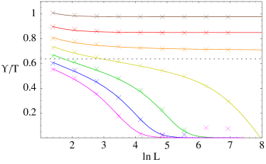
(a) Dimensionless helicity modulus $u=\Upsilon/T$ as a function of system size. The curves are solutions of the scaling equations, Eq. (3), chosen to fit the data (crosses). The dashed line is $\Upsilon/T=\tfrac{2}{\pi}$.

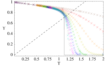
(b) Helicity modulus as a function of temperature. The black curve is $\Upsilon(L=\infty,T)$ obtained by FSS. The dashed line is $\Upsilon=\tfrac{2}{\pi}T$.

Figure 2: Finite-size scaling. The crosses are Monte Carlo results for the helicity modulus $\Upsilon(L,T)$ of a 4x4-modulated XY model with $J_{w}=0$ and $J_{s}=4J_{\rm avg}$, for $T=0.9,1.0,...,1.5$ in units of $J_{\rm avg}$ and $L=4,8,...1024$.

The XY model has the following classical Hamiltonian:

$$\mathcal{H}_{\text{XY}}[\theta] =-\sum_{\left\langle ij\right\rangle}J_{ij}\cos(\theta_{i}-\theta_{j})$$ (1)

where $i,j$ are site labels, $J_{ij}$ are nearest-neighbour couplings, and $\theta_{\mathbf{x}}$ are real-valued phase (angle) variables. We choose the couplings $J_{ij}$ so as to preserve $\sum_{ij}J_{ij}$. This leaves the zero-temperature properties of the system unchanged, such as the helicity modulus $\Upsilon(T=0)$ and the energy $U(T=0)$. We consider here only two-dimensional models.

We are interested in how to optimize the transition temperature, and to study this we focus on the behavior of the helicity modulus $\Upsilon(T)$ of the XY model, which is directly proportional to the superfluid stiffness $n_{s}$ of a phase-dominated superconductor. by We study this quantity via Monte Carlo simulations on square lattices, where $\Upsilon(T)$ can be calculated using

$$\Upsilon =\frac{1}{2V}\left\langle\sum_{\left\langle ij\right\rangle}J_{ij}\cos(\theta_{i}-\theta_{j})-\beta\bigg{[}\sum_{\left\langle ij\right\rangle}J_{ij}\sin(\theta_{i}-\theta_{j})\bigg{]}^{2}\right\rangle.$$ (2)

We use the Wolff cluster algorithmwolff1989 , which is the fastest serial algorithm for our purposes. The $\theta$ variables are stored and manipulated as two-vectors to avoid trigonometric function calls.

In order to obtain reliable estimates of $T_{c}$, we have performed finite-size scaling (FSS) on $\Upsilon(L,T)$ in the following manner. The KT transition can be described by a two-parameter scaling flow kosterlitz1974 ; nelson1977 ; jose1977 ; schultka-manousakis for the dimensionless helicity modulus $u=\Upsilon/T$ and the ‘vortex fugacity’ $y$,

$$\frac{du}{dl} =-4\pi^{3}u^{2}y^{2},\quad\frac{dy}{dl}=(2-\pi u)y,$$ (3)

where $l=\ln L$ is the length scale. This pair of differential equations can be solved numerically, given initial values $u(l_{0})=u_{0}$ and $y(l_{0})=y_{0}$ (where $l_{0}$ is some reference length scale). For each temperature $T$, we choose $u_{0}$ and $y_{0}$ so as to obtain a good fit of $u(l)$ to the Monte Carlo data for the available system sizes, $4\leq L\leq 1024$ (see Fig. 2(a)). We then integrate the differential equations all the way to $l=\infty$. This gives $u(\infty)$ and hence the helicity modulus in the infinite-size limit $\Upsilon(T,L=\infty)$, shown in Fig. 2(b).

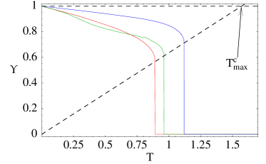
Figure 3: $\Upsilon(T,L=\infty)$ for 2D XY models. The red curve is for the homogeneous 2D XY model. The green curve is for a 4x4 modulation with $J_{\text{strong}}=3.4$ and $J_{\text{weak}}=0.2$. The blue curve is for a 4x4 modulation with $J_{\text{strong}}=4$ and $J_{\text{weak}}=0.$ The dashed line is $\Upsilon=\frac{2}{\pi}T$; the arrow indicates a theoretical upper bound on $T_{c}$, $T^{c}_{\text{max}}=\frac{\pi}{2}J_{\rm avg}$.

Our most important result is that by redistributing the bond strengths of an XY model in certain inhomogeneous patterns, it is possible to increase $T_{c}$. As a concrete example of how this comes about, we show how the shape of the helicity modulus curve vs. temperature is changed by introducing inhomogeneity. In Fig. 3, we show our simulations of $\Upsilon(T)$, extrapolated to infinite system size $L\rightarrow\infty$, for a 2D inhomogeneity of the type shown in Fig. 1(b), using $\lambda=4a$ where $a$ is the underlying lattice constant. In the blue and green curves of Fig. 3, the coupling constant $J_{ij}$ has been made stronger on the darker lines in Fig. 1(b), ($J_{\rm strong}$), and weaker on the lighter lines ($J_{\rm weak}$). We compare these to the uniform case (the red curve) with $J$ set equal to the spatial average of $J_{\rm weak}$ and $J_{\rm strong}$, $J=J_{\rm avg}\equiv(J_{\rm strong}+(\lambda-1)J_{\rm weak})/\lambda$. Thus for all curves shown in Fig. 3, the zero temperature helicity modulus $\Upsilon(T=0)$ and the zero temperature free energy are the same.

In the uniform case, it is known that $T_{c}=0.8929J$ schultka-manousakis ; hasenbusch2005 , and that the low temperature slope of the helicity modulus $\Upsilon^{{}^{\prime}}(0)=1/4$ classphs ; roddick-stroud . The green curve in Fig. 3 shows the helicity modulus for $J_{\rm strong}=3.4$ and $J_{\rm weak}=0.2$. In this case, the transition temperature is enhanced by $8\%$ above the homogeneous case. For the case of extreme inhomogeneity with $J_{\rm strong}=4$ and $J_{\rm weak}=0$ (the blue curve), the transition temperature is $25\%$ higher than in the uniform case. The shape of the green curve demonstrates the separation of energy scales that happens with inhomogeneity. Notice that at the very lowest temperatures, the green curve is dominated by the long-wavelength average of the coupling constants, and the low temperature linear slope of the helicity modulus is identical to that of the homogeneous case. As temperature is raised, the slope increases in magnitude, as the weak plaquettes become disordered. Then, at a higher temperature, the slope approaches that of the blue curve, indicating that at higher temperatures the helicity modulus is dominated by $J_{\rm strong}$. It is this shallower high temperature slope which causes the helicity modulus to overshoot the homogenous $T_{c}$, and leads to an inhomogeneity-induced enhancement of the transition temperature.

For 2D patterns like those in Fig. 1(b), the enhancement of the transition temperature increases with $\lambda$, as shown by the green curve of Fig. 4. However, the enhancement is constrained by the zero temperature helicity modulus. Even in the presence of inhomogeneity, in 2D the system remains in the KT universality class, and the helicity modulus has a universal jump at the transition such that $\Upsilon(T_{c})=0.6365T_{c}$. Since thermal fluctuations introduce disorder, $\Upsilon(T_{c})<\Upsilon(T=0)$, so that $T_{c}/\Upsilon(0)\leq 1.57$, or equivalently, $T_{c}/T_{c0}\leq 1.76$. This theoretical upper bound on $T_{c}$ is illustrated in Fig. 3. That is, although the zero temperature properties of the system may be used as a predictor of the transition temperature, $T_{c}=A\Upsilon(T=0)$, the constant $A$ is non-universal. In fact, $A=T_{c}/\Upsilon(0)$ may be useful for characterizing the degree of inhomogeneity: it increases from $0.89$ for the uniform XY model up to a theoretical maximum of $1.57$. For a 2D system, a large measured value of this ratio may indicate substantial inhomogeneity. (An increase in this ratio may also indicate higher dimensionality.classphs )

We have also considered one-dimensional modulations, like those in Fig. 1(a). Since this type of inhomogeneity drives the system towards more one-dimensional physics where a phase transition is forbidden by the Mermin-Wagner theorem, the transition temperature decreases, as shown in Fig. 4. Hence the enhancement of $T_{c}$ is not additive — the effect of a 2D modulation is not double that of a 1D modulation.

Fig. 4 also shows the effect of inhomogeneity in the Ising model, for comparison. Inhomogeneous Ising models may be described by the Hamiltonian

$$\mathcal{H}_{\text{Ising}}[\sigma] =-\sum_{\left\langle ij\right\rangle}J_{ij}\sigma_{i}\sigma_{j},\quad\sigma_{i}=\pm 1.$$ (4)

As with the XY model, we restrict ourselves to two dimensions. For the purpose of studying different length scales of inhomogeneity, we focus on an extreme type of inhomogeneity with $J_{\rm weak}=0$, and $J_{\rm strong}=\lambda J_{\rm avg}$. Such patterns correspond to ‘decorated’ lattices. By integrating out all doubly-coordinated spins (that is, by applying the so-called decorated-iteration transformation, $J_{\text{eff}}=\tanh^{-1}(\tanh J_{1}\tanh J_{2})$), one can reduce a decorated lattice to a primitive lattice and thus obtain an exact expression for its $T_{c}$ (Eq. (5)). (Unfortunately, the decoration-iteration transformation for XY models involves an infinite set of Fourier components of the potentialjose1977 and it does not lead to exact results for $T_{c}$.)

In Fig. 4, we show the effect of extreme inhomogeneity (i.e., with $J_{\rm weak}=0$) on the transition temperatures in Ising and XY models. We use the maximum value of $J_{\rm strong}=\lambda J_{\rm avg}$, because for a given wavelength $\lambda$, this gives the largest enhancement of $T_{c}$ while conserving the average coupling $J_{\rm avg}$. While we are interested primarily in superconductors with small superfluid density, which can be captured with an XY model, we also show results for the Ising model, for which results can be obtained analytically as described above. Fig. 4 shows the effect of a purely 1D modulation, as a function of distance $\lambda$ between strong bonds $J_{\rm strong}$, chosen so as to preserve the zero temperature, long wavelength properties of the system. The pattern of coupling constants is shown in Fig. 1(a). In the Ising case, the transition temperature is unchanged by this procedure. In the XY case, the transition temperature decreases monotonically with $\lambda$.

The effect of a 2D modulation is shown in Fig. 4. Again, parameters are chosen so as to preserve the zero temperature properties of the system. Fig. 1(b) shows the pattern of coupling constants. Here, the transition temperature in the Ising case increases as

$$T_{c}=\frac{2\lambda J_{\rm avg}}{\sinh^{-1}[{\rm csch}(\frac{1}{\lambda}\sinh^{-1}1)]}~{}.$$ (5)

One of the occurrences of lambda in this equation is due to taking $\lambda$ bonds in parallel, to form“bundles”, and the other occurrence is due to taking $\lambda$ bundles in series. For XY models, the transition temperature also increases monotonically with modulation length $\lambda$. In this case there is an upper bound, set by the zero temperature properties of the system, as shown in Fig. 3. That is, the maximum enhancement of $T_{c}$ possible with this type of inhomogeneity in an XY model is $76\%$.

In conclusion, we have shown that certain types of inhomogeneity can increase the transition temperature of Ising and XY models. Specifically, two-dimensional modulations of the coupling constants that preserve the spatial average coupling increase the transition temperature over that of the uniform case. One-dimensional modulations depress the transition in XY models, and leave the transition temperature unchanged in Ising models. Our results for 2D XY models may indicate that certain types of inhomogeneity can result in an enhancement of superconductivity in systems with low superfluid density.

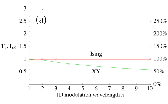
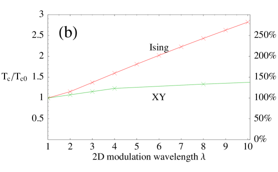
Figure 4: Critical temperatures $T_{c}$ of the lattices depicted in Fig. 1(a) and 1(b), as a function of the wavelength of the inhomogeneity.

It is a pleasure to thank S. A. Kivelson, E. Manousakis, and D. Stroud for helpful discussions. This work was supported by Purdue University (YLL), Research Corporation (YLL), and by the Purdue Research Foundation (EWC). EWC is a Cottrell Scholar of Research Corporation. This research was supported in part through computing resources provided by Information Technology at Purdue-the Rosen Center for Advanced Computing, West Lafayette, Indiana.

References

- (1) I. Martin, D. Podolsky, and S. A. Kivelson, Phys. Rev. B, 72, 060502(R) (2005).
- (2) K. Aryanpour, et al., Phys. Rev. B, 73, 104518 (2006).
- (3) E. Arrigoni and S. A. Kivelson, Phys. Rev. B, 68, 180503(R) (2003).
- (4) U. Wolff, Phys. Rev. Lett., 62, 361 (1989).
- (5) J. M. Kosterlitz, Journal of Physics C: Solid State Physics, 7, 1046 (1974).
- (6) D. R. Nelson and J. M. Kosterlitz, Phys. Rev. Lett., 39, 1201 (1977).
- (7) J. V. José, L. P. Kadanoff, S. Kirkpatrick, and D. R. Nelson, Phys. Rev. B, 16, 1217 (1977).
- (8) N. Schultka and E. Manousakis, Phys. Rev. B, 49, 12071 (1994).
- (9) U. Wolff, J. Phys. A, 38, 5869 (2005).
- (10) E. W. Carlson, S. A. Kivelson, V. J. Emery, and E. Manousakis, Phys. Rev. Lett., 83, 612 (1999).
- (11) E. Roddick and D. Stroud, Phys. Rev. Lett., 74, 1430 (1995), linear-T dependence of SF density.
- (12) E. Dagotto, Science, 309, 257 (2005).
- (13) E. W. Carlson, V. J. Emery, S. A. Kivelson, and D. Orgad, Concepts in High Temperature Superconductivity, Springer-Verlag (2004), in The Physics of Superconductors, Vol. II, ed. J. Ketterson and K. Benneman.
- (14) S. Bose, P. Raychaudhuri, R. Banerjee, P. Vasa, and P. Ayyub, Phys. Rev. Lett., 95, 147003 (2005).
- (15) M. E. Fisher, 7, 10 (1966).
- (16) Y. L. Loh and E. W. Carlson, accepted by Phys. Rev. Lett. (2006).