Numerical evidence for relevance of disorder in a Poland-Scheraga DNA denaturation model with self-avoidance:
Scaling behavior of average quantities.

Abstract

We study numerically the effect of sequence heterogeneity on the thermodynamic properties of a Poland-Scheraga model for DNA denaturation taking into account self-avoidance, i.e. with exponent $c_{p}=2.15$ for the loop length probability distribution. In complement to previous on-lattice Monte Carlo like studies, we consider here off-lattice numerical calculations for large sequence lengths, relying on efficient algorithmic methods. We investigate finite size effects with the definition of an appropriate intrinsic length scale $x$, depending on the parameters of the model. Based on the occurrence of large enough rare regions, for a given sequence length $N$, this study provides a qualitative picture for the finite size behavior, suggesting that the effect of disorder could be sensed only with sequence lengths diverging exponentially with $x$. We further look in detail at average quantities for the particular case $x=1.3$, ensuring through this parameter choice the correspondence between the off-lattice and the on-lattice studies. Taken together, the various results can be cast in a coherent picture with a crossover between a nearly pure system like behavior for small sizes $N\lesssim 1000$, as observed in the on-lattice simulations, and the apparent asymptotic behavior indicative of disorder relevance, with an (average) correlation length exponent $\nu_{r}\geq 2/d\>(=2)$.

PACS: 64.60.Fr     Equilibrium properties near critical points, critical exponents
PACS: 82.39.Pj     Nucleic acids, DNA and RNA bases
PACS: 02.60.Cb    Numerical simulation, solution of equations

1 Introduction

The discovery of the DNA double-helical structure, some 50 years ago, motivated the elaboration of the helix-coil model to account for the separation of the two strands, on physical bases [1, 2, 3]. The importance of this model from the biological point of view is obvious, since processing of the genetic information involves precisely the separation of the strands. Of course, under physiological conditions, the opening of the double-helix is not under the effect of temperature, but the differential stabilities in DNA sequences, as revealed by helix-coil analysis, could be sensed by biological effectors, such as proteins, under various types of constraints. The successful development of the helix-coil denaturation model required appropriate elaborations for the physics and the algorithmics, allowing accurate tests through comparisons with experimental data (melting curves). This field, very active in the sixties and seventies, has benefited recently from a renewed interest both from the biological side, for example in the context of genomic analysis, and from the physics side, notably in relation with questions relevant to the order of the transition in the homogeneous case and the effect of sequence heterogeneity. In the light of these still debated issues, both from the theoretical and the numerical points of view, the main focus of the present work is the numerical investigation of the relevance of disorder in a realistic DNA denaturation model à la Poland-Scheraga, in which self-avoidance between loops and the rest of the chain is also taken into account. In what follows, before further detailing the particular system considered and the open questions, we first recall briefly the general background in terms of biological models, numerical methods and previous results.

Basics for DNA denaturation: DNA denaturation is an entropy driven transition, in which at some critical temperature $T_{c}$ the energy loss $\Delta E$ with the opening of base pairs is compensated by the entropic gain $T\Delta S$ associated with the increased number of configurations accessible to the separated single strands. Experimentally, it is found that $T_{c}$ depends on different factors, in particular the $pH$ of the solution and the GC composition of the sequence, related to the ratio of the Guanine-Cytosine, GC, pairs to the Adenine-Thymine, AT, pairs. For homogeneous sequences, for $pH\sim 7$, typical values for $T_{c}$ are $T_{c,{GC}}\sim 110\>^{0}C$ and $\>T_{c,{AT}}\sim 70\>^{0}C$, respectively for GC and AT cases. Such differences reflect of course the fact that the pairing of Guanine to Cytosine involves three hydrogen bonds whereas that of Adenine to Thymine involves only two.

For a given biological sequence of length $N$, here identified, following AT and GC pairs, by the coupling energies $\{\epsilon_{i},i=1,\dots,N\}$, the denaturation transition can be followed with UV absorption. Correspondingly, the fraction $\theta_{\epsilon}(T,N)$ of closed base pairs, which is the order parameter of the transition in the thermodynamic limit $N\rightarrow\infty$, can be measured in such experiments based on differential absorptions for closed and open base pairs. The resulting curves display usually multi-stepped structures, with abrupt variations on small (sequence-depending) temperature ranges around $T_{c}$. Therefore, for a biological sequence of fixed length, the finite size order parameter $\theta_{\epsilon}(T,N)$ varies from zero to one (associated with complete denaturation), with a sequence-dependent behavior. Accordingly, the derivative with respect to temperature, $-d\theta_{\epsilon}(T,N)/dT$, displays typically a series of sharp peaks.

From the theoretical point of view, modeling DNA denaturation was essentially following two main directions: 1) for biological applications, in relation with melting experiments (sixties, seventies), sequence-dependent algorithmic elaborations for the handling of realistic physical models [2, 4, 5], concerning notably the representation of denaturation loops, and, 2) for the study of the underlying physics, detailed characterizations of the properties for pure systems, neglecting sequence-specificity [6, 7, 8, 9, 10, 11, 12, 13, 14, 15, 16].

Physics of DNA denaturation for homogeneous sequences: DNA denaturation is understandable in the framework of almost unidimensional systems [18], and it is therefore associated with a peculiar kind of transition. In fact, the first models displayed no thermodynamic singularity [2], as they corresponded to $1d$ Ising models with only short-range (nearest-neighbor) interactions, with open and closed base pair states represented by an Ising spin. It was subsequently shown, notably by Poland and Scheraga [6] (PS, in what follows), that the observed denaturation behavior can indeed be described in terms of a simple $1d$ model, the helix-coil model, that consists of alternating regions of contiguous open base pairs (coiled regions or loops) and double-stranded ones (helical segments). In this model the transition in the thermodynamic limit is made possible through the adoption of appropriate long-range entropic weights for the single-stranded loops.

More recently, several other models have been considered and studied, using in particular more realistic potential forms between base pairs [8, 9]. Since sharp transitions are observed experimentally, with abrupt changes in $\theta_{\epsilon}(T,N)$ on small temperature ranges, it is expected that a model, accounting correctly for such results, should undergo a first order transition in the pure case. Indeed, this point has been studied rather extensively recently [3, 8, 9, 10, 11, 12, 13, 14, 15, 16, 17]. In particular, it was demonstrated [10] that the transition is of first order in pure PS models in which excluded volume effects for loops are not only with themselves, but also with the rest of the chain. Notably, with the probability distributions for loops with lengths $l$ at the critical point following a power law, $P(l,T_{c})\propto 1/l^{c_{p}}$, the transition is of first order for $c_{p}$ exponents larger than 2 [6, 7, 18] (see also [3]). It was shown that in three dimensions, with the two strands described as self-avoiding walks (SAWs), the value for the exponent is $c_{p}\simeq 2.15$ [10, 12, 14, 15]. In comparison, $c_{p}=3/2$ for random walk (RW) loops [6] and $c_{p}=1.76276(6)$ for SAW loops, with excluded volume interactions with the rest of the chain neglected [7, 19].

Biological and algorithmic backgrounds for sequence-specific DNA denaturations: The algorithmic problem was initially encountered for the implementation of sequence-specific calculations allowing notably experimental/theoretical comparisons in the study of melting curves. It seemed natural, in the beginning, to resort to transfer matrix formalisms as developed in physics because of the Ising-type formulation of the problem [2]. Indeed, neglecting loop-entropy long-range effects, the calculation of the partition function for a sequence of size $N$ can be expressed simply as the product of $N$ $2$x$2$ matrices. The extension to realistic models was at first handled through extended transfer matrices, of sizes growing up to $N$x$N$, for the proper description of interactions throughout the lengths of the sequences [2]. Because of calculation burdens associated with such matrix sizes, alternative formulations were sought for the implementation of realistic models with affordable computation times. Representing the culmination of a series of developments, through some twenty years, an appropriate algorithmic solution was proposed in 1977 by Fixman and Freire [4] (FF method), in which calculation efficiency was not at the price of oversimplifications in the physics, but relied instead on the numerical representation of the long-range effect as a multiexponential function. In this formulation, the time complexity for the evaluation of a complete denaturation map for a sequence of length $N$ is essentially proportional to $N$. This reduced complexity is to be compared with the intrinsic complexity of the model scaling as $N^{3}$, if we were to consider exact one-way calculations along the sequence.

In this background, no generalizations were proposed for the ideas in the FF for a long period of time, possibly because of the formulation of this method in the prolongation of an algorithm by Poland [20], expressed in the rather specialized context of conditional probabilities recursions specific to the linear DNA helix-coil model. As a matter of fact, the only applications of the FF concerned the implementation of the algorithms in computer programs, for DNA melting calculations (such as in the POLAND [21] or in the MELTSIM programs [22]). However, upon revisiting the original derivations, it appears that the idea associated with the multiexponential representation, relying on the fundamental property of exponential function, corresponds to a powerful concept amenable to many generalizations for realistic models with long-range effects. Accordingly, based on explicit partition function calculations, the SIMEX (SIMulations with EXponentials) method was first derived as a reformulation of the FF for the linear helix-coil model [5], with further generalizations to higher-order models involving several, mutually coupled, long-range effects [23, 24]. For such systems, with two or more long-ranges, the reductions of complexities by several orders of magnitudes can be associated with calculation times reduced by million folds. The basic concepts for higher-order models were originally illustrated with a circular DNA helix-coil model-problem involving two long-range contributions [23]. The corresponding principles were further transposed to a linear helix-coil model with non-symmetrical loops [24].

On the experimental side, linear helix-coil models were successfully compared with experimental denaturation curves [22]. In the beginning, one of the motivations in the elaboration of DNA denaturation models was to ask the question of possible relations between genetics (coding/non-coding) and physical (helix/coil) segmentations, because of the importance of the separation of the two strands in the processing of the genetic information. With little genomic sequences available at the end of the seventies and beginning of eighties, no clearcut conclusions were reached for such relations. More recently, with the availability of complete genomes, it was possible to resume such investigations on much larger bases, demonstrating variable correspondences between the two types of segmentations, depending on the genomes [25, 26, 27, 28]. For genomes with very sharp correlations it was even possible to propose ab initio gene identification methods purely on physical bases [26].

Physics of DNA denaturation with disorder: On the physical side, DNA denaturation models are associated with important open questions such as, notably, the relevance of sequence-heterogeneity for the thermodynamic limit behavior. At the beginning of the seventies, it was noted by Poland and Scheraga [2] that “sequence heterogeneity dramatically broadens the transition”, but it is only recently that such problem has been addressed on more rigorous bases and the transition in disordered PS models with $c_{p}>2$ was also investigated [29, 30, 31, 32, 33, 34]. Indeed, in the homogeneous case, such systems exhibit peculiar first order transitions characterized by a diverging correlation length, and it is therefore not clear to which extent general theoretical results on the effect of disorder [35, 36, 37] can be applied. The question has been addressed both with analytical [32, 33, 34] and numerical approaches, with either off-lattice [29, 30] or on-lattice [31] implementations in this latter case. It appears however hard to reconcile these various results. The off-lattice studies of [29, 30], involving very large chain lengths, suggest a peculiar transition, of first order as in the pure case but not obeying usual finite size scaling and exhibiting two different correlation length exponents, associated respectively with typical and average quantities. On the other hand, the Monte Carlo like numerical simulations in [31], limited to small chain lengths, agree with a second order transition in the presence of disorder, though it was not possible to rule out completely a transition still of first order. Finally, from the analytical standpoint, under quite general hypotheses encompassing PS models with $c_{p}>2$, it was shown that the transition is expected to be at least of second order and possibly smoother [32, 33, 34].

In the background above, in addition to their relevance to experimental DNA denaturation, PS models with sequence heterogeneity represent interesting toy-models for addressing general open questions relative to the proprieties of random fixed points. The detailed study of such systems could also help elaborating the correct approaches to be used in the interpretation of data on disordered models. In this direction, we perform here a numerical analysis of a disordered PS model with $c_{p}=2.15$. Relying on appropriate algorithmic formulations (SIMEX) we consider long sequences. With the definition adopted for the model, and the choices for the parameter values, the calculations are made directly comparable with previous on-lattice results [31]. In addition, the observed behavior should be also related to that found in the previous off-lattice studies of a different disordered PS model with $c_{p}=2.15$ [29, 30], in which the same multiexponential representation for the long-range loop entropy law was adopted.

Our findings show the existence of very strong corrections to scaling. Moreover it appears that, for a given size, the effect of disorder is qualitatively described by an appropriately defined intrinsic length scale $x$ depending on model parameters. These observations provide a possible explanation for the discrepancies between previous results [29, 30, 31], as well as for an apparent dependence of the evaluated critical exponents on model parameters noted in [31]. In fact, in the frame of the picture proposed here, the size at which the effect of disorder becomes evident could diverge exponentially with $x$. More precisely, for the value $x=1.3$ chosen for the present detailed study, it is possible to observe a crossover between a nearly pure system like behavior, consistent with the one observed in simulations [31], and the apparent asymptotic one. With corrections to scaling taken into account, the model clearly displays a smooth transition, corresponding to a value for the correlation length exponent $\nu_{r}\geq 2/d\>(=2)$. Nevertheless, since our results refer to average quantities, they do not rule out the possibility suggested in [29, 30, 38, 39] of a transition governed by two different correlation lengths. The analysis for the clarification of this point is left for a forthcoming work [40].

2 Models à la Poland-Scheraga

2.1 The pure case and the role of the exponent $c_{p}$

Pure PS models for DNA denaturation are described in a rather extensive literature, and in particular the ingredients which make the transition of first order are discussed in several recent works [3, 10, 11, 12, 13, 14, 15, 16]. Here we will only recall results for linear PS models with symmetric loops, in which one fully takes into account self-avoidance through an appropriate choice of the loop length distribution probability exponent $c_{p}$.

The position of a base pair along the sequence is labeled by $i$ ($i=1,\dots,N$) and its configurational state is represented by $s_{i}$, with $s_{i}=1$ for a closed pair and $s_{i}=0$ for an open pair. In the corresponding on-lattice representation, the two strands in the model can be visualized as two interacting RWs with the same origin in $d$ dimensions. A pair is in the closed state if and only if the two bases are in the same position $i$ along the two strands and occupy the same lattice point [13] (RW-DNA). One can write the canonical partition function for the system in the form:

$$Z_{N}=\sum_{E}{\cal N}(E)e^{-\beta\>E},$$ (1)

where ${\cal N}(E)$ is the number of configurations with the same total energy $E$ and $\beta=1/T$ is the inverse temperature, taking Boltzmann constant $k_{B}=1$ for simplicity.

The contribution of a single base pair in the closed state to the total energy $E$ is $\Delta E=-\epsilon$, independent from the position $i$ in the pure case. The number of configurations of a closed segment of length $n$ increases as $\mu^{n}$ and therefore its contribution to the total entropy $S(E)=\log{\cal N}(E)$ is $\Delta S=n\log\mu$. Here $\mu$ is a parameter of the model, interpretable as the on-lattice connectivity constant ($\mu=2d$ for $d$-dimensional RWs on a cubic lattice). A denatured region of length $l$ is associated with a single-stranded loop of length $2l$, and the corresponding number of configurations is given by $\mu^{2l}/(2l)^{c_{p}}$. The factor $1/(2l)^{c_{p}}$ takes into account the fact that the two separated chains have to meet again at some distant point, and the relation $c_{p}=d/2$ holds for $d$-dimensional RWs.

Assuming that the first and the last base pairs are always coupled, a given configuration of the system is described by the lengths of the closed segments $\{n_{j}\}$ and by those of the denatured loops $\{l_{k}\}$, with $\sum_{j}n_{j}+\sum_{k}(l_{k}-1)=n_{tot}+l_{tot}=N$. Its energy is $E=-\epsilon\sum_{j}n_{j}=-\epsilon n_{tot}$, only depending on $n_{tot}$. Therefore, in the partition function, the degeneracy factor ${\cal N}(E)$ includes both the entropic contribution of segments $\mu^{n_{tot}}$ and that of loops $\mu^{2l_{tot}}\prod_{k}{1}/{(2l_{k})^{c_{p}}}$, the latter being to be summed over all the possible sets $\{l_{k}>2\}$ associated with a given total length $l_{tot}=\sum_{k}(l_{k}-1)$. Correspondingly, the partition function can be also written as:

$$Z_{N} = e^{2N\log\mu}\sum_{n_{tot}}e^{n_{tot}(\beta\epsilon-\log\mu)}\sum_{\{l_{k}>2\}}\delta(n_{tot}+l_{tot}-N)\prod_{k}{\frac{1}{(2l_{k})^{c_{p}}}}=$$ (2)

$$= e^{2N\log\mu}\sum_{\{n_{j}\}}\sum_{\{l_{k}>2\}}\delta(n_{tot}+l_{tot}-N)\prod_{j}e^{n_{j}(\beta\epsilon-\log\mu)}\prod_{k}{\frac{1}{(2l_{k})^{c_{p}}}}$$

It can be noted that the factor $e^{2N\log\mu}$ contributes an additive constant to the entropy and it is therefore not relevant for the description of the thermodynamics of the system. In what follows, we study properties of $Z^{*}_{N}=Z_{N}/e^{2N\log\mu}$. Accordingly, the number of loops of length $l_{k}$ is taken equal to $1/(2l_{k})^{c_{p}}$ and a negative contribution to the entropy $\Delta S=-\log\mu$ is associated to each base pair in the closed state. It is seen qualitatively that the possible change in the thermodynamic limit behavior occurs at the temperature for which $\beta_{c}\epsilon\sim\log\mu$. From the last expression in (2) it is moreover clear that, in the computation of the grand canonical partition function ${\cal Z}$, the contributions of helical segments and loops are decoupled and one obtains a geometric series [2, 6, 7, 12, 18]:

$${\cal Z}=\sum_{N}z^{N}Z_{N}=\sum_{\rho}\left\{\left[\sum_{n=1}^{\infty}z^{n}e^{n(\beta\epsilon-\log\mu)}\right]\left[\sum_{l=2}^{\infty}{\frac{z^{l}}{(2l)^{c_{p}}}}\right]\right\}^{\rho}=\frac{{\cal Z}_{S}{\cal Z}_{L}}{1-{\cal Z}_{S}{\cal Z}_{L}},$$ (3)

where we introduced the fugacity $z$ and ${\cal Z}_{S}$ and ${\cal Z}_{L}$ refer to the segment (helical) and loop (coil) grand partition functions respectively:

$${\cal Z}_{S} = \sum_{n=1}^{\infty}z^{n}e^{n(\beta\epsilon-\log\mu)}=\frac{ze^{(\beta\epsilon-\log\mu)}}{1-ze^{(\beta\epsilon-\log\mu)}},$$ (4)

$${\cal Z}_{L} = \sum_{l=2}^{\infty}\frac{z^{l}}{(2l)^{c_{p}}}.$$ (5)

Since the behavior for $N\rightarrow\infty$ is dictated by the fugacity value $z^{*}$ corresponding to the pole nearest to the origin, the system undergoes a phase transition when a critical temperature $T_{c}$ is found below which the zero of the denominator becomes smaller than the smallest pole of the numerator. The possibility of the transition and its order both depend on the value of the exponent $c_{p}$ [2, 6, 7, 12, 18]. In detail, for $c_{p}<1$ there is no thermodynamic singularity, whereas for $c_{p}>1$ the following situations must be distinguished: a smooth transition for $1<c_{p}<3/2$ with a specific heat exponent $\alpha_{p}<0$, a second order transition for $3/2\leq c_{p}\leq 2$ and finally a first order transition for $c_{p}>2$. In fact, these distinctions can be understood considering the properties of ${\cal Z}_{L}$, i.e. those of the distribution probability of the loop length at the (possible) critical point $P(l,T_{c})=1/(2l)^{c_{p}}$:

$$\sum_{l}P(l,T_{c}) = \infty\mbox{ for }c_{p}\leq 1$$ (6)

$$\sum_{l}lP(l,T_{c}) = \left\{\begin{array}[]{lcl}\infty&\mbox{ for }&c_{p}\leq 2.\\ const&\mbox{ for }&c_{p}>2\end{array}\right.$$ (9)

In the case $c_{p}\leq 2$, the mean length $\langle l\rangle$ for loops at the critical point diverges and the system exhibits large coiled regions, in which most of the bases are involved. On the contrary, for $c_{p}>2$, the mean loop length at $T_{c}$ is finite and correspondingly it is possible to show that the density of closed base pairs $\theta(T,N)=\langle n\rangle/N$, and therefore the energy density, varies abruptly in the thermodynamic limit, from the value zero at high temperatures to a finite value at $T_{c}$. In detail, when approaching the critical point from the low temperature (helical) phase, one finds [2, 6, 7, 12, 18]:

$$\theta(T)\equiv\lim_{N\rightarrow\infty}\frac{1}{N}\sum_{i=1}^{N}\langle s_{i}\rangle\propto\left\{\begin{array}[]{lcl}(T_{c}-T)^{\frac{2-c_{p}}{c_{p}-1}}&\mbox{ for }&1<c_{p}\leq 2\\ (T_{c}-T)^{0}&\mbox{ for }&c_{p}>2\\ \end{array}\right.$$ (10)

For example, the RW-DNA model in three dimensions exhibits a second order transition with $\alpha_{p}=0$, since $c_{p}=3/2$, whereas in five dimensions it undergoes a first order transition, since $c_{p}=5/2$, as confirmed both by exact computations of thermodynamic quantities and by on-lattice numerical simulations [13].

2.2 Exponent value $c_{p}=2.15$

All interactions between different loops and helical segments are neglected in classical calculations of the grand canonical partition functions for helix-coil models. It is possible to account for self-avoidance of each loop with itself through the appropriate choice of the exponent $c_{p}=1.76276(6)$ [7, 19], corresponding roughly to the value adopted usually for comparisons with experimental data [22]. More recently, it was demonstrated that self-avoidance of the loops with the rest of the chain can be also taken into account, and that intriguingly the pure PS models exhibit first order transitions in this case [10, 11, 12]. The exponent $c_{p}$, corresponding to a self-avoiding loop embedded in a self-avoiding chain, can be predicted from conformal theory results [41], and in particular it was found that $c_{p}\simeq 2.15$ in three dimensions, the transition being of first order also in $d=2$. It is notable that such determination provides the appropriate value of $c_{p}$ to be used as an input in off-lattice calculations.

In the Monte Carlo like simulations, one studies an on-lattice model (SAW-DNA) in which self-avoidance is completely taken into account, by considering two interacting SAWs, with two monomers allowed to occupy the same lattice point if and only if their positions along the two chains are identical, thus representing complementary base pairs [13]. In the pure $3d$ case, it was found that this system exhibits a first order transition, with the maximum of the specific heat diverging linearly with the chain length. It was subsequently shown [14, 15] that the value of the exponent describing the probability distribution for the loop lengths at the critical point is in perfect agreement with the theoretical prediction, $c_{p}\simeq 2.15$. An off-lattice pure PS model with $c_{p}=2.15$ was also studied numerically [42], finding the same scaling behavior than in $3d$ SAW-DNA, apart from the strong finite size corrections which appear to be more important in the on-lattice situation.

Even though of first order, the transition is characterized by a diverging correlation length, which can be identified from the behavior of $P(l,T)$ [10, 12, 15]:

$$P(l,T)\propto\frac{e^{-l/\xi(T)}}{(2l)^{c_{p}}}$$ (11)

with

$$\xi(T)\propto(T-T_{c})^{-\nu_{p}}\mbox{ for }T\rightarrow T_{c}^{-}.$$ (12)

where $\nu_{p}=1$ for $c_{p}>2$ and $\nu_{p}=1/(c_{p}-1)$ for second order (or smoother) transitions. It can also be predicted that the free energy density $f(T)$ takes the value zero in the high temperature phase and that it behaves proportionally to $1/\xi(T)$ for $T\rightarrow T_{c}^{-}$, leading again to the behavior of the energy density and of the order parameter for different $c_{p}$ values given in (10). Therefore, the hyperscaling relation $\alpha_{p}=2-\nu_{p}$ is clearly fulfilled, both for $c_{p}\leq 2$ and for the first order ($\alpha_{p}=1$) case.

2.3 Effect of disorder: previous results

Disorder is introduced to account for sequence-heterogeneity, with parameter values depending on the chemical nature of base pairs (AT or GC) at a given position along a sequence. There are a few studies on the effect of disorder on general properties of DNA denaturation models in which self-avoidance is neglected [43, 44, 45, 46, 47]. Previous numerical works on disordered models à la PS was mainly for comparison of the predictions with experimental data and genetic signals [22, 25, 26, 27, 28] and for the study of the effect of base pair mismatches [24], where one usually takes also into account the stacking contributions, with the coupling energies depending on the chemical nature of base pairs at positions $i$ and $i+1$. For comparisons with experimental melting curves, it is moreover necessary to take into account the possibility for complete dissociation of the two strands in the molecule [2, 48]. We also notice that biological sequences exhibit long-range correlations and strong variability in GC compositions, both according to genomes and within chromosomes. Letting aside for the present such sophistication, we sum up some recent results for simple disordered models à la PS with self-avoidance, such as those considered in off-lattice [29, 30] and on-lattice [31] studies, which allow nevertheless to capture essential features of the effect of disorder.

In these various works, disorder enters only through the position dependent contribution of a closed base pair to the total energy. In detail, the $\{\epsilon_{i}\}$ are quenched random variables distributed following a binomial probability, corresponding to GC composition equal to 1/2:

$$P(\epsilon)={\frac{1}{2}}\left[\delta(\epsilon-\epsilon_{AT})+\delta(\epsilon-\epsilon_{GC})\right],$$ (13)

with $\epsilon_{AT}<\epsilon_{GC}$. One is interested in the thermodynamic properties of the quenched free energy density:

$$f(T)=\lim_{N\rightarrow\infty}f_{\epsilon}(T,N)=\lim_{N\rightarrow\infty}\overline{f_{\epsilon}(T,N)}=-\lim_{N\rightarrow\infty}{\frac{1}{\beta N}}\overline{\log Z_{N,\epsilon}},$$ (14)

where, as usual, $\overline{(\cdot)}$ denotes the average over disorder and $f_{\epsilon}(T,N)$ is a self-averaging quantity in these models [32].

Generally speaking it is known, from the theoretical point of view, that disorder can modify very significantly the fixed point of a system, and therefore its critical exponents. In what follows, the notations with subscripts $p$ and $r$ refer to the (possibly different) pure and random system fixed points, respectively. A series of results [35, 36, 37], and notably the well known Harris criterion [35], demonstrate that disorder is relevant as soon as the specific heat exponent fulfills the condition $\alpha_{p}>0$. Correspondingly, in the presence of disorder, the transition becomes smoother and it is in particular expected that $\alpha_{r}\leq 0$, i.e., from the hyperscaling relation, a correlation length exponent $\nu_{r}\geq 2/d$ [49, 50, 51]. It is however important to stress that these results are obtained essentially for magnetic systems and it is not clear to which extent they are relevant to the case here considered, concerning interacting polymers undergoing a first order transition characterized by a diverging correlation length.

An analysis in terms of pseudo-critical temperatures [52] was applied recently to disordered PS models with different $c_{p}$ values [29, 30, 38, 39, 53, 54]. In these studies, an appropriate sample-dependent $T_{c}(\epsilon,N)$ was defined and measured, looking in particular at the associated probability distribution. The results point towards irrelevance of disorder for $c_{p}=3/2$, corresponding to the marginal case $\alpha_{p}=0$. On the contrary, relevance of disorder was found for $c_{p}>3/2$. Importantly, peculiar behavior was observed for the value $c_{p}=2.15$, whereas the situation appears to be clear for $c_{p}=1.75$. Indeed, for $c_{p}=1.75$, compatible estimates for $\nu_{r}\sim 2.7\>(>2/d=2)$ were obtained from the scaling of the average pseudo-critical temperature $T_{c}(N)$ and from that of (the square root of) its fluctuations $\delta T_{c}(N)$. In the case $c_{p}=2.15$, instead, a scaling of the average critical temperature $T_{c}(N)\sim 1/N$ was reported, suggesting a still first order transition with exponent $\nu_{r,1}=1$. However it was also found a scaling for the fluctuations following $\delta T_{c}(N)\sim 1/N^{1/2}$, which was associated to a different exponent $\nu_{r,2}=2\>(=2/d)$. It was then suggested [29, 30, 38, 39] that these observations are compatible with a system still exhibiting a first order transition but in which scaling laws are no more fulfilled, characterized by two different correlation lengths: a typical one, $\xi_{1}\sim 1/|T-T_{c}|$, describing the behavior of a typical sample in the thermodynamic limit, with $\nu_{r,1}=1$, and an average one, $\xi_{2}\sim 1/(T-T_{c})^{2}$, describing the behavior of average quantities, dominated by rare fluctuations, with $\nu_{r,2}=2/d=2$. The resulting two-sided scenario is therefore that disorder is irrelevant to the typical sample and, in the same time, the obtainment of the $\nu_{r,2}$ value is in agreement with the theoretical expectations [49, 50, 51].

By contrast, usual finite size scaling analysis of Monte Carlo like simulations results on a $3d$ disordered SAW-DNA model (DSAW-DNA) [31], suggested a transition governed by an (average) correlation length exponent $\nu_{r}\simeq 1.2$. However, in this study, average energy curves were observed to cross at the same point within the errors in the estimations, and accordingly the possibility $\nu_{r}=1=\nu_{p}$ could not be completely ruled out. The findings were further confirmed by the analysis of the behavior of $\overline{P_{\epsilon}(l,T)}$ at the critical point, which led to the compatible value $c_{r}\simeq 1.9\simeq 1+1/\nu_{r}$ when considering the largest sizes and taking into account the presence of a finite correlation length. But again, particularly with the smallest chain lengths, estimations $c_{r}>2$, still compatible with a first order transition, were obtained. It is noticeable that the affordable sizes in Monte Carlo like studies are significantly smaller (factors of order $\sim 2000$) than the sequence lengths accessible to off-lattice recursive canonical partition function calculations for PS models.

Finally, in recent theoretical works based on a probabilistic approach [32, 33, 34], it was shown for a general class of interacting polymer models that the transition becomes at least of second order in the presence of disorder. The frame of this approach covers the PS models with $c_{p}>3/2$, including the case $c_{p}>2$ with corresponding first order transition in the pure system. Accordingly, these conclusions are expected to also cover the $3d$ DSAW-DNA case. Following such studies, it is expected that $\nu_{r}\geq 2$ both for average and typical quantities, though the possibility of different correlation lengths is not ruled out [34]. On the other hand, according to other theoretical results in which self avoidance is neglected [46, 47], disordered models à la PS could undergo a definitely smoother transition, corresponding to an essential singularity in the free energy.

2.4 A possible scenario for the finite size behavior

Before presenting our numerical findings, it is worth discussing qualitative features expected, at fixed chain lengths $N$, for the behavior of disordered PS models. As previously recalled, disorder should be relevant to these models as soon as $c_{p}>3/2$. Moreover, on general grounds, one can argue that the behavior of a system near the transition point is governed by given critical exponents which do not depend on model details. Correspondingly, one would expect that both the form of $P(\epsilon_{i})$ and the precise choices for the parameters (here $R=\epsilon_{GC}/\epsilon_{AT}$, $\mu$ and GC composition) should not correspond to different thermodynamic limit singularities. On the other hand, such choices could have strong influence on finite size effects.

The disordered PS model in [29, 30] and the $3d$ DSAW-DNA in [31] involve the same $c_{p}=2.15$, either as a direct input for the recursive calculations or as consequence of the implementation of self-avoidance in the simulated model. Nevertheless, there is a first noticeable difference between the two systems studied, as the off-lattice calculations were inspired from a wetting transition model [54], in which it is forbidden for two consecutive elements to be in the closed state simultaneously (i.e., in our notation, if $s_{i}=1$ then $s_{i+1}=0$). Also the connectivity constant $\mu$ is not the same, since it was fixed to the value $\mu=2$ in [29, 30], whereas it is an output of the model in the on-lattice simulations, and one finds $\mu\simeq 4.7$ for SAWs on a $3d$ cubic lattice. In addition, the two studies involved significantly different $R$ values. In [29, 30] the choice $R\simeq 1.098$ was adopted, for obtaining a critical temperature ratio $T_{c,GC}/T_{c,AT}$ close to the experimental value. On the other hand, in [31], the value $R=2$ was studied in detail and the values $R=4$ and $R=\infty$ (corresponding to the choice $\epsilon_{GC}=1$ and $\epsilon_{AT}=0$) were also considered. In the latter study, preliminary results suggested that the (average) correlation length exponent $\nu_{r}$ could increase with $R$, ranging from $\nu_{r}\simeq 1.18$ for $R=2$ to $\nu_{r}\simeq 1.33$ for $R=\infty$.

For proper understanding of these findings, and for a qualitative analysis of the expected finite size behavior, it can be important to consider in some detail the potential key role of rare regions in the generated sequences. Indeed, the possible presence of such regions, of large enough size, can explain the presence of strong corrections to scaling, which could therefore depend both on model details and on the precise choice for the parameters. It can be noted that temperature and disorder appear only in the $\pi_{i}=\exp[{s_{i}(\beta\epsilon_{i}-\log\mu})]$ terms in the partition function, which are clearly invariant under the transformation $(\epsilon_{i}\rightarrow\alpha\epsilon_{i},\>T\rightarrow\alpha T)$. Moreover, in the pure system, the transition occurs around the temperature $T_{c,{p}}\sim\epsilon/\log\mu$, at which the energetic contribution for the two bound chains is of the same order than the entropic loss. In the presence of disorder, for a given sequence, it is expected to observe the multi-step behavior in $\theta_{\epsilon}(T,N)$ displayed by experimental DNA denaturation curves. This results from the presence of regions with different local contents in terms of GC to AT ratios, associated accordingly with different local melting temperatures.

In the simplest extreme case, one imagines two regions $A$ and $B$, of about the same length $L$, completely dominated by AT and GC compositions respectively. In such situation, the local transition in region $A$ is driven by $\epsilon_{AT}$ energies, with local critical temperature $T_{c,loc}(A)\sim T_{c,{AT}}\sim\epsilon_{AT}/\log\mu$, whereas the local transition in region $B$ is associated with the higher local critical temperature $T_{c,loc}(B)\sim T_{c,{GC}}\sim\epsilon_{GC}/\log\mu\sim RT_{c,loc}(A)$. In this illustrative example, for a given temperature, the contributions in the partition function of total $\pi^{tot}_{A,B}$ factors corresponding to the configurations with base pairs in the closed state, will be significantly different for $A$ and $B$ regions. One obtains, for $T=T_{c,loc}(B)$ and $s_{i}=1\>\>\forall i\in A,B$:

$$\pi^{tot}_{A} = \prod_{i\in A}\pi_{i}=\exp\left[{L(\beta_{c,loc}(B)\epsilon_{AT}-\log\mu)}\right]\sim O(1),$$

$$\pi^{tot}_{B} = \prod_{i\in B}\pi_{i}=\exp\left[{L(\beta_{c,loc}(B)\epsilon_{GC}-\log\mu)}\right]\sim\exp(-L/x).$$ (15)

Since, whereas $\beta_{c,loc}(B)\epsilon_{GC}-\log\mu\sim 0$, one has

$$\beta_{c,loc}(B)\epsilon_{AT}-\log\mu\sim-\log\mu\frac{R-1}{R}\equiv-\frac{1}{x},$$ (16)

defining the parameter $x$. From these expressions it is possible to argue that the larger the value of $L$ with respect to $x$ the more the effect of disorder will be felt by the finite size system, i.e. the difference between the weights of configurations corresponding to closed $A$ and $B$ regions in the partition function will be higher. On the other hand, the probability for such an extreme case in a particular sequence of size $N$ is quite small. With the choice for $P(\epsilon)$ in (13), large $N$ and $L$ values and $2^{L}\gg N\gg L$, the probability of $L$ contiguous elements of the same type is simply $\sim N/2^{L}$. Therefore this probability, though approaching 1 in the thermodynamic limit for any finite $L$, becomes rapidly negligible with increasing $L$ for fixed chain length $N$. Following these considerations, for the finite size system to feel the effect of disorder, the chain lengths necessary for observing rare regions with $L\gg x$ could be not reachable for large $x$ values. For more quantitative analysis, at least in the extreme case considered, let us suppose that at the length scale $N_{1}$ a region of size $L_{1}$ is observed for the parameter value $x_{1}$, such that $L_{1}/x_{1}\gg 1$, with non negligible probability $N_{1}/2^{L_{1}}$. Then, in order to make the same observation for $x_{2}>x_{1}$, it will be necessary to consider length scales of order $N_{2}\sim N_{1}\exp\left[(x_{2}/x_{1}-1)L_{1}\log 2\right]$, thus involving exponential increases with the ratio $x_{2}/x_{1}$ for the sequence lengths $N$.

For attempting to understand the role of the long-range loop entropic effect, one can impose that, at the temperature $T_{c,loc}(B)$, the weight of the configuration associated with region $A$ in the closed state is significantly smaller than that of the configuration associated with an open region corresponding to a single loop (of size $L$), getting the condition $L/x\gg c_{p}\log L$. Correspondingly, one can argue that, with increasingly larger $c_{p}$ values, increasingly larger rare region lengths will be necessary for observing cooperative melting behavior at different temperatures. Moreover, the considered extreme case seems particularly appropriate for a qualitative description when $c_{p}>2$. Here, the first order character of the transition in the pure system and the corresponding favored formation of small loops suggests that larger differences of local AT to GC content ratio are necessary for obtaining different local melting temperatures.

In conclusion, important finite size corrections to scaling are expected qualitatively, which could in particular depend strongly on the parameter $x$ introduced above, involving both the energy ratio $R$ and the connectivity constant $\mu$. Specifically, the effect of disorder on the behavior of the system could become evident only for chain lengths diverging exponentially with $x$. This parameter seems therefore to play the role of an intrinsic length scale for the rare regions, corresponding to the logarithm of an intrinsic length scale for the system itself.

Setting aside other differences, the parameter choices in [29, 30] correspond to $x\sim 15$, whereas in [31] they give $x\simeq 1.3$. It is accordingly possible that results in the two studies can be explained following the described picture, on the basis of the underlying finite size effects. It is nevertheless to be noted that in [29, 30] very large sequences, up to $N\sim 2000000$, were considered. The present qualitative picture could anyway explain the observations in [31], for an apparent dependence of $\nu_{r}$ on $R$, as an increase in $R$ at fixed $\log\mu$ amounts to a decrease in $x$. It is possible that the chain lengths $N\leq 800$ affordable in the simulations were not large enough and that also the value $\nu_{r}\simeq 1.33$ obtained with $R=\infty$ was affected by finite size corrections to scaling, being therefore to be interpreted as a lower bound for the (asymptotic) $\nu_{r}$.

3 Numerical study

3.1 Details of the model

We consider the disordered PS model, with $c_{p}=2.15$, described by the canonical partition function:

$$Z^{*}_{N,\epsilon}=\sum_{\{s_{i}\}}\prod_{i}e^{s_{i}(\beta\epsilon_{i}-\log\mu)}\prod_{k}{\frac{1}{(2l_{k})^{c_{p}}}},$$ (17)

where $\prod_{k}$ runs over all the loop lengths $l_{k}>2$, associated with a given configuration of the $\{s_{i}\}$. Importantly, here and in the following we only impose the condition $\sum_{k}(l_{k}-1)+\sum_{i}s_{i}=l_{tot}+n_{tot}\leq N$, thus allowing for free ends, with separated strands not involved in a loop at one end-extremity of the sequence. Such free-ends are not expected to modify the thermodynamic limit behavior [10, 12, 29], but the high temperature phase of the model will consist accordingly of two strands linked only at $i=1$ (instead of a large loop, for a system with both extremities required to be in the coupled state). This so-called bound-unbound ($bu$) model corresponds more closely to the one studied usually in on-lattice simulations [13, 14, 15, 31], and it was also adopted in [29, 30]. We notice that the factor $\mu^{2(N-l_{tot}-n_{tot})}$ cancels out when looking at $Z^{*}=Z/\mu^{2N}$.

In the present study, we are moreover implicitly adopting the value $\sigma=1$ for the cooperativity factor, where the parameter $\sigma$ gives a measure for the barrier to overcome for the initiation of a loop opening. In realistic sequence-specific calculations [22, 25, 26, 27, 28], one uses typically $\sigma=O(10^{-5})$. It is however not clear what choice for $\sigma$ is appropriate when $c_{p}=2.15$ since in experimental/theoretical comparisons an exponent $c_{p}\sim 1.8$ is generally taken and in a recent study [55] it was suggested that the values for $\sigma$ and $c_{p}$ should vary in parallel in order to reproduce correctly experimental melting curves. We note that small $\sigma$ values could increase corrections to scaling, whereas this parameter is not expected to influence the thermodynamic properties.

Disordered PS models can be solved numerically by writing down recursive equations for the partition function with a SIMEX scheme [4, 5, 23, 24], taking into account efficiently the long-range entropic loop weights. A basic idea in the recursive scheme is that the forward partition function $Z^{f}_{\epsilon}(\rho+1)$, which accounts for all configurations up to position $\rho+1$ along the sequence with both base pairs at positions $i=1$ and $i=\rho+1$ in the closed state ($s_{1}=s_{\rho+1}=1$), can be obtained from $Z^{f}_{\epsilon}(\rho)$:

$$Z^{f}_{\epsilon}(\rho+1)=\exp({\beta\epsilon_{\rho+1}-\log\mu})\left[Z^{f}_{\epsilon}(\rho)+\sum_{\rho^{\prime}=1}^{\rho-1}\frac{Z^{f}_{\epsilon}(\rho^{\prime})}{[2(\rho-\rho^{\prime}+1)]^{c_{p}}}\right].$$ (18)

We can similarly write down the equation for the backward partition function:

$$Z^{b}_{\epsilon}(\rho-1)=\exp({\beta\epsilon_{\rho-1}-\log\mu})\left[Z^{b}_{\epsilon}(\rho)+\sum_{\rho^{\prime}=\rho+1}^{N}\frac{Z^{b}_{\epsilon}(\rho^{\prime})}{[2(\rho^{\prime}-\rho+1)]^{c_{p}}}+1\right],$$ (19)

with the last term in the equation above corresponding to the free-end configuration ($s_{i}=0$ for $i>(\rho-1)$). The canonical partition function for the complete chain of length $N$ is given by:

$$Z^{*}_{N,\epsilon}=\sum_{\rho=1}^{N}Z^{f}_{\epsilon}(\rho)=Z^{b}_{\epsilon}(1),$$ (20)

where the forward sum takes into account the free-ends. With these calculations one obtains in particular the probability for a base pair at position $i$ (along the sequence of length $N$) to be in the closed state as:

$${\cal P}_{\epsilon}(i,T,N)=\langle s_{i}\rangle=\frac{Z^{f}_{\epsilon}(i)Z^{b}_{\epsilon}(i)}{Z^{*}_{N,\epsilon}\exp({\beta\epsilon_{i}-\log\mu})},$$ (21)

where the division with $\exp({\beta\epsilon_{i}-\log\mu})$ is to rectify the double counting of the corresponding factor (involved both in $Z^{f}_{\epsilon}$ and in $Z^{b}_{\epsilon}$).

3.2 Measured observables

For a given disorder sequence $\{\epsilon_{i},\>i=1,\dots,N\}$, at fixed chain length $N$ and temperature $T$, we can derive from the ${\cal P}_{\epsilon}(i,T,N)=\langle s_{i}\rangle$ (21) quantities of interest such as the density of closed AT base pairs $\theta_{AT,\epsilon}$ (respectively GC, $\theta_{GC,\epsilon}$), the total density of closed base pairs $\theta_{\epsilon}$ and the energy density $e_{\epsilon}$:

$$\theta_{AT,\epsilon}(T,N) = \frac{1}{N}\left\langle\sum_{i\in AT}s_{i}\right\rangle=\frac{1}{N}\sum_{i\in AT}{\cal P}_{\epsilon}(i,T,N),$$ (22)

$$\theta_{GC,\epsilon}(T,N) = \frac{1}{N}\left\langle\sum_{i\in GC}s_{i}\right\rangle=\frac{1}{N}\sum_{i\in GC}{\cal P}_{\epsilon}(i,T,N),$$ (23)

$$\theta_{\epsilon}(T,N) = \theta_{AT,\epsilon}(T,N)+\theta_{GC,\epsilon}(T,N)$$ (24)

$$e_{\epsilon}(T,N) = -\left[\epsilon_{AT}\theta_{AT,\epsilon}(T,N)+\epsilon_{GC}\theta_{GC,\epsilon}(T,N)\right].$$ (25)

We can also consider the specific heat $c_{\epsilon}$ as well as the derivative of the density of opened base pairs $c_{\theta,\epsilon}$, which is relevant to experimental determinations:

$$c_{\epsilon}(T,N) = \frac{1}{T^{2}}\frac{de_{\epsilon}(T,N)}{dT}$$ (26)

$$c_{\theta,{\epsilon}}(T,N) = -\frac{1}{T^{2}}\frac{d\theta_{\epsilon}(T,N)}{dT}.$$ (27)

Since $R\neq 1$, the energy density $e_{\epsilon}$ and the order parameter $\theta_{\epsilon}$ can exhibit different behaviors, and accordingly such can be also the case for $c_{\epsilon}$ and $c_{\theta,{\epsilon}}$. In the same direction we consider also the susceptibility, obtained as:

$$\chi_{\epsilon}(T,N) = \frac{1}{N}\left[\left\langle\left(\sum_{i=1}^{N}s_{i}\right)^{2}\right\rangle-\left\langle\left(\sum_{i=1}^{N}s_{i}\right)\right\rangle^{2}\right]=$$ (28)

$$= \frac{1}{\beta}\left[\frac{d\theta_{AT,\epsilon}(T,N)}{d\epsilon_{AT}}+\frac{d\theta_{GC,\epsilon}(T,N)}{d\epsilon_{GC}}+\frac{d\theta_{AT,\epsilon}(T,N)}{d\epsilon_{GC}}+\frac{d\theta_{GC,\epsilon}(T,N)}{d\epsilon_{AT}}\right],$$

providing interestingly a possibility for checking numerical accuracy in the computations, from the fulfillment of the equality ${d\theta_{AT,\epsilon}(T,N)}/d\epsilon_{GC}={d\theta_{GC,\epsilon}(T,N)}/d\epsilon_{AT}$.

We study moreover the behavior of the (non-normalized) loop length probability distribution:

$$P_{\epsilon}(l,T,N)={\cal N}(l)\sum_{i=1}^{N-l-1}\frac{Z^{f}_{\epsilon}(i)Z^{b}_{\epsilon}(i+l+1)}{Z^{*}_{N,\epsilon}}$$ (29)

with ${\cal N}(l)=1/(2l)^{c_{p}}$, independent from the disorder sequence. Therefore we introduce the quantity:

$$P^{*}_{\epsilon}(l,T,N)=(2l)^{c_{p}}P_{\epsilon}(l,T,N).$$ (30)

noting that in the pure model $P^{*}(l,T,N)\propto\exp({-l/\xi(T,N)})$ (see (11)) and correspondingly $P^{*}(l,T,N)\rightarrow const$ for $T\rightarrow T_{c}^{-}$.

As a first step in the analysis of such data, we will check the validity of standard finite size scaling for quantities averaged over disorder. With the usual definition of the critical exponents and $y=(T-T_{c})N^{1/\nu_{r}}$, one expects:

$$\overline{e_{\epsilon}(T,N)} \sim N^{1/\nu_{r}-1}\tilde{e}(y)$$ (31)

$$\overline{c_{\epsilon}(T_{c},N)} \sim N^{2/\nu_{r}-1}\tilde{c}(y),$$ (32)

$$\overline{\theta_{\epsilon}(T,N)} \sim N^{-\beta_{r}/\nu_{r}}\tilde{\theta}(y)$$ (33)

$$\overline{\chi_{\epsilon}(T,N)} \sim N^{\gamma_{r}/\nu_{r}}\tilde{\chi}(y),$$ (34)

where it is possible to find $\beta_{r}/\nu_{r}\neq 1-1/\nu_{r}$ and $\gamma_{r}/\nu_{r}\neq 2/\nu_{r}-1=\alpha_{r}/\nu_{r}$. For the average loop length probability distribution, we still look for a behavior at the critical point described by a power law as in the pure case:

$$\overline{P_{\epsilon}(l,T_{c},N)}\propto 1/l^{c_{r}},$$ (35)

and therefore

$$\overline{P^{*}_{\epsilon}(l,T_{c},N)}\propto l^{c_{p}-c_{r}}.$$ (36)

Interestingly, based on this relation, it should be particularly simple to seek numerical evidence for $c_{r}\neq c_{p}$.

3.3 Computational details

We resort to the SIMEX scheme [5, 23, 24], based explicitly on partition function evaluations, instead of recursions for specific conditional probabilities as in [4]. Besides this conceptual difference (important for generalizations, notably to higher-order models), for the simple helix-coil model in linear molecules, as considered here, the reduction of the computational complexity by one order of magnitude in the SIMEX method relies on the numerical representation of the long-range effects in the model as a sum of $N_{S}$ exponentials, as already formulated in the FF method. The other important ingredient in the FF, also implemented straightforwardly in the SIMEX, corresponds to a forward-backward scheme as described in Section 3.1, classical in dynamic programming and associated with an additional order of magnitude reduction in complexities. For the linear case, the complexities for a complete probability map calculation reduce overall from $N^{3}$ (for a one-way progressive treatment) to $N_{S}N$.

In order to make the scheme operational in practice, it is necessary to obtain appropriate numerical representations for long-range effects as sums of exponentials. The general numerical problem associated with the analysis of multiexponential functions is notoriously a delicate one. It covers two distinct -in principle- situations, concerning either identifications or approximations, the relevant case for the present study. In the identification situation, it is necessary to recover the correct number of exponentials, and of course the correct associated parameters, from curves (usually experimental) supposed to be of multiexponential type for theoretical reasons. A general solution to this problem is provided by the Padé-Laplace method [56], requiring no a priori hypotheses for the identification of components in sums of general exponentials (real and/or complex). This formulation encompasses, and generalizes, in a unified frame, a series of solutions since Prony’s method and the so-called method of moments [57]. Even though originally formulated as an identification approach, the numerical application of the Padé-Laplace method to power-law functions (such as for loop-entropies here) revealed an identification-like behavior in this approximation problem, in the sense that, for given maximal long-range lengths, a fixed number of significant exponential components are obtained. For example, for a series of biologically-oriented studies, an approximation of $1/l^{1.95}$ with $N_{S}=14$ exponentials was shown to be appropriate (with further refinements of the parameters with least-squares procedures) [25]. In the present study, in order to be in strictly comparable conditions with this respect, we adopt the numerical representation of $1/l^{2.15}$ with $N_{S}=15$ exponentials in [29].

For the numerical computation of the recursive equations for the forward and backward partition functions, it is moreover necessary to avoid underflow/overflow problems. For this purpose different schemes can be implemented [5, 24], in order to normalize the numerators and denominators the ratios of which are involved in the evaluation of probabilities (21). We consider here the normalization described in [24], based on the introduction of free energy like quantities for the handling of the logarithms of $Z^{f}_{\epsilon}$ and $Z^{b}_{\epsilon}$. The details of the implementations are provided in the Appendix, along with the description of boundary conditions.

We study extensively the case $x=R/[\log\mu(R-1)]=1.3$, using the same energies and connectivity constant as in [31]: $R=2$ and $\log\mu\simeq\log\mu_{SAW}\simeq 1.54$, in three dimensions. We consider sequence lengths ranging between $N=100$ and $N=20000$. For $x=1.3$, such $N$-values appear to be large enough both for the clarification of the thermodynamic limit behavior and for the study of corrections to scaling. On the other hand, the numerical computations are reasonably fast up to this length, which makes it possible to consider closely spaced temperatures and to obtain correspondingly, with negligible numerical errors, quantities related to derivatives, such as in particular the values of the maxima of the specific heat. In detail, for given chain lengths, we consider ${\cal N}_{T}=250$ different $T$-values, equally spaced in intervals $[T_{min}(N),T_{max}(N)]$ around the corresponding $T_{c}(N)$, evaluated roughly from the position of the maximum of the average specific heat in some preliminary results. For the different chain lengths, the number of samples ${\cal N}_{s}(N)$ as well as the $T_{min}(N)$ and $T_{max}(N)$ temperatures are detailed in [Tab. 1].

$N$	${\cal N}_{s}(N)$	$T_{min}(N)$	$T_{max}(N)$
100	2000	0.95	1.2
200	2000	0.95	1.2
500	2000	1.0	1.16
750	1000	1.0	1.16
1000	1000	1.0	1.15
2500	1000	1.02	1.14
5000	1000	1.02	1.14
7500	1000	1.04	1.12
10000	600	1.04	1.14
15000	500	1.04	1.12
20000	500	1.04	1.12

Table 1: Tabulation of the chain lengths $N$, the number of samples ${\cal N}_{s}(N)$ and the range of temperatures $[T_{min}(N),T_{max}(N)]$ in the numerical computations. For each disordered sequence ${\cal N}_{T}=250$ equally spaced temperatures, in the corresponding intervals, are considered.

It was checked in particular that with the various choices above the errors on the maximum of specific heat and of susceptibility were both consistently smaller than fluctuations between samples. Without any loss of generality we set in all calculations $\epsilon_{AT}=1$, i.e. temperature is in $\epsilon_{AT}$ unities. The evaluation of the susceptibility is obtained by numerical derivations with respect to $\epsilon_{AT}$ and $\epsilon_{GC}$ (see (28)), with $\delta\epsilon_{AT}=\beta\cdot 10^{-4}$ and $\delta\epsilon_{GC}=R\delta\epsilon_{AT}$, which ensures the desired numerical accuracy at all temperatures. Finally, in all calculations the errors on average quantities are computed from sample-to-sample fluctuations.

4 Results and discussion

4.1 Given sample-sequence and different $x$ values

We consider first the qualitative behavior of the model for a given sample-sequence of length $N=10000$, with different $x=R/[\log\mu(R-1)]$ values. Results shown in this Section are obtained with a particular disorder configuration. It was however checked that the corresponding qualitative observations are also valid with various arbitrarily chosen sequences. In order to cover different significant situations, the following values for the parameter $x$ were considered: $x=2,\>1.3,\>1.4,\>0.7$, respectively. Notably, the choice $x=2$ is for comparisons with the results in [29, 30]. In detail, we used the same $R=1.098$, and we set in addition $\log\mu\simeq 5.55$, for obtaining close critical temperatures in the pure case. The choice $x=1.3$ is for compatibility with the conditions in [31], and accordingly we set in this case $R=2$ and $\log\mu\simeq 1.54$. On the other hand, the choice of the close value $x\simeq 1.4$ is following parameters setting usual in comparisons with experimental results [22, 25, 26, 27]. In this latter case, the value for $x$ is not related to a large $R$ value, but rather to a large average $\log\mu\simeq 12.35$ (in $k_{B}$ unities). It can be noticed that typically used coupling energies lead to $R\simeq 1.062$, as obtained by averaging over the different stacking energies for neighbor base pairs $\epsilon_{i,i+1}$. Finally, for clarification of potential differences resulting from choices of large $R$ or alternatively large $\mu$ values, $x\simeq 0.7$ was retained as corresponding to the two choices for ($R$, $\log\mu$) couples: $R\simeq 1.062$, $\log\mu\simeq 24.5$ (case $a$); and $R\simeq 18.38$, $\log\mu\simeq 1.54$ (case $b$).

We plot in [Fig. 1] the susceptibilities $\chi_{\epsilon}(T,x,N)$ for the sample-sequence for the different $x$ values. We observe that the results depend strongly on $x$. However, the shapes of the curves obtained with $x=1.3$ and $x=1.4$ appear to be strikingly similar. Moreover, also the two curves corresponding to the two different cases associated with $x=0.7$ (case $a$ and case $b$) are qualitatively similar.

Figure 1: Susceptibility curves for a given sample-sequence of length $N=10000$ and different $x$ values (see text).

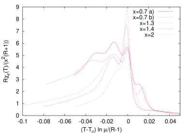
Figure 2: Scaled susceptibility for a given sample-sequence of length $N=10000$ and different $x$ values. $\chi_{\epsilon}R/[x^{2}(R+1)]$ data are plotted as function of $[T-T_{c}(\epsilon,x,N)]\log\mu/(R-1)$, with $T_{c}(\epsilon,x,N)$ the temperature associated with the absolute maximum of susceptibility. In the case $a$ with the value $x=0.7$, specific choice was needed for defining the pseudo-$T_{c}$, and we looked in this case to correspondence of positions of the peaks with the other curves, by taking it as the temperature of the second maximum.

The results here are in agreement with the overall picture given in Section 2.4, with indications for an $x$-dependent finite size behavior. The extreme case considered there, with pure AT and GC regions, is clearly a very rough approximation of a typical sequence. It is nevertheless clear that the parameter $x$ appears to capture some essential ingredients of the model.

For more quantitative analysis, we note that for $N\rightarrow\infty$ one expects a transition temperature close to $T_{c}^{\infty}\sim(T_{c,{AT}}+T_{c,{GC}})/2\sim(R+1)/(2\log\mu)$. For a given finite sequence, a pseudo-critical temperature $T_{c}(\epsilon,x,N)$ must be adopted, as the critical temperature is not well defined. Here we take as $T_{c}(\epsilon,x,N)$ the temperature associated with the highest maximum value for susceptibility [52]. In particular, with such a choice, we find that the behavior of $\chi_{\epsilon}(T,x,N)$ displays some scaling when plotted as function of $[T-T_{c}(\epsilon,x,N)]T_{c}(\epsilon,x,N)/(R-1)$, for different $R$ and $x$ values. We present in [Fig. 2] correspondingly scaled $\chi_{\epsilon}$ data (also multiplied by the factor $R/[x^{2}(R+1)]$, for obtaining close behaviors in the high temperature phase).

This figure further makes evident the dependence on $x$ for finite size systems. The results suggest that, at fixed length scale $N$, for large $x$, and in particular here already for the value $x=2$, the system exhibits typically only one very sharp peak. This observation should be related to the fact that the probability of large enough rare regions is negligible (though one could still encounter such a case when considering a large number of sequences), and the system behaves essentially as a pure model with $\epsilon=(\epsilon_{AT}+\epsilon_{GC})/2=(R+1)/2$. For smaller $x$ values, we observe on the contrary an increasing number of peaks, with decreased sharpness. This finding is coherent with the qualitative picture following which, with increasingly smaller $x$ values, rare regions with increasingly smaller lengths $L$ are sufficient in order to observe multistep behaviors, since the relevant quantity should be the ratio $L/x$. Nevertheless, for the smallest considered value $x=0.7$, obtained with two different parameters choices, we observe the same number (four) of peaks, but the position with respect to the other peaks for the absolute maximum of the curve is shifted for $x=0.7\>a$ as compared to the corresponding one for $x=0.7\>b$ and the larger $x$ values. This confirms that the introduced $x$ describes the finite size behavior only approximately.

The changes in the behavior of a typical sample, as described above, are also expected at larger sequence sizes for a given $x$-value, since this parameter appears to behave as (the logarithm of) an intrinsic length scale of the system. Some numerical evidence in this direction was already given in [31] for the on-lattice DSAW-DNA, where the qualitative analysis of the specific heat suggested the appearance of multi-peaked curves only for large enough $N$-values, and an increasing number of peaks in typical sequences as function of $N$. Here we obtain the same qualitative results for the value $x=1.3$ studied in detail. Nevertheless, detailed quantitative bases for such conclusions are left for future work, with an extensive study of the finite size effects for different $x$ values.

It is to be emphasized that in the suggested picture it is the behavior of the typical finite size sample which is expected to change when varying $x$, and therefore one would not expect different typical and average correlation lengths in the thermodynamic limit, though the sizes necessary for confirming this hypothesis could be out of reach for large $x$ values. An analysis in terms of pseudo-critical temperatures is clearly necessary to distinguish between this situation and the alternative one proposed in [29, 30, 38, 39], which is left to a forthcoming work [40].

4.2 Behavior of average quantities

In what follows, we investigate the behavior of average quantities for $x=1.3$ (obtained by setting $R=2$ and $\log\mu=1.54$). The average energy density $\overline{e_{\epsilon}(T,N)}$ and the average closed base pair density $\overline{\theta_{\epsilon}(T,N)}$, for different chain lengths, are represented in [Fig. 3]. It is clear that the system undergoes a phase transition in the thermodynamic limit, with the energy density and the order parameter going from zero at high temperature to finite values below $T_{c}$. We can moreover observe from [Fig. 3] very similar behaviors for the two quantities (apart from the sign difference) and we expect to find, as a consequence, $\beta_{r}=\nu_{r}-1$ and $\gamma_{r}=\alpha_{r}=2-\nu_{r}$. We have also checked that the average densities of closed AT $\overline{\theta_{AT,\epsilon}(T,N)}$ and GC $\overline{\theta_{GC,\epsilon}(T,N)}$ base pairs exhibit qualitatively similar behaviors.

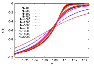
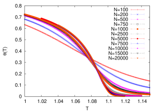
Figure 3: Averaged energy density $\overline{e_{\epsilon}(T,N)}$ and averaged total density of closed base pairs $\overline{\theta_{\epsilon}(T,N)}$, for various chain lengths, plotted as functions of temperature.

Nevertheless, the data do not agree with the corresponding expected scaling laws (see (31) and (33)), making clear the presence of strong corrections to the asymptotic behavior. Even though it is therefore difficult to evaluate the critical exponents, the fact that the curves do not cross at the same point (as particularly evident for the largest sizes) suggests a transition with (an average) $\nu_{r}>1\>(=\nu_{p})$. More in detail, the energy density and the order parameter appear to converge both towards functions which are continuously vanishing at the critical point and possibly also differentiable, which would imply a transition at least of second order.

Still better evidence for a smooth transition comes from the average specific heat $\overline{c_{\epsilon}(T,N)}$ data, plotted in [Fig. 4]. One can notice from this figure that the maximum appears to diverge with the chain length for the smallest sizes, but saturates for larger $N$-values, as expected for a critical point characterized by $\alpha_{r}\leq 0$, i.e. $\nu_{r}\geq 2/d\>(=2)$. Interestingly, the qualitative behavior for chain lengths smaller than $\sim 1000$ appears to be similar to the one found in [31]. This observation suggests that the on-lattice DSAW-DNA and the off-lattice disordered PS model considered could exhibit the same kind of finite size effects, also supporting the hypothesis that the value $\nu_{r}\sim 1.2$ obtained from the Monte Carlo like numerical simulations represents a lower bound for the average correlation length critical exponent.

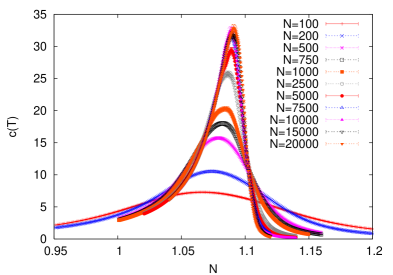
Figure 4: Average specific heats $\overline{c_{\epsilon}(T,N)}$, for the chain lengths considered, plotted as functions of temperature.

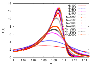
Figure 5: Averaged susceptibilities $\overline{\chi_{\epsilon}(T,N)}$, for the chain lengths considered, plotted as functions of temperature.

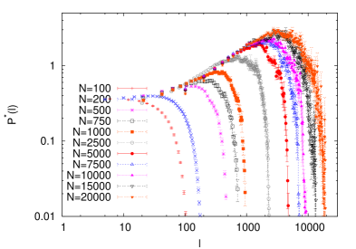
Figure 6: Average $\overline{P^{*}_{\epsilon}(l,T_{c}(N),N)}=(2l)^{c_{p}}\overline{P_{\epsilon}(l,T_{c}(N),N)}$, for the chain lengths considered, plotted as functions of the loop lengths $l$ at temperatures $T_{c}(N)$, corresponding to maxima of average specific heat. Normalization factors are arbitrarily chosen in order to make values comparable at small $l$.

We find a very similar behavior for the susceptibility $\overline{\chi_{\epsilon}(T,N)}$, represented in [Fig. 5], as well as for the derivative with respect to the temperature of the total density of closed base pairs $\overline{c_{\theta,\epsilon}(T,N)}$ (not shown). These findings further suggest that these quantities, as well as the energy and the order parameter, are described also in the disordered case by the same critical exponents. Again, it is difficult to evaluate the exponents by applying standard finite size scaling analysis to the data, because of the obvious presence of strong corrections to the expected laws (here (32) and (34)).

Finally, [Fig. 6] displays data for $\overline{P^{*}_{\epsilon}(l,T_{c}(N),N)}$ (see (30)) at the size-dependent critical temperatures $T_{c}(N)$, identified here with the temperatures associated with the maximum of the average specific heat. We note also in this case a strongly $N$-dependent behavior. In particular, the considered quantity is nearly constant in the range $1\ll l\ll N$ for the smallest sizes, whereas for the largest ones, expected to be the most meaningful, it is increasing with $l$ rather linearly (on logarithmic scale) on a wide ranged interval, which should mean that the expected power law representation (35) is valid, but with $c_{r}\ll c_{p}$.

We notice that the observed strong $N$-dependence of averaged quantities and the fact that data do not obey usual scaling laws on the whole $N$-range studied is in agreement with the qualitative picture given in Section 2.3, clearly suggesting that, at fixed $x$, the effect of disorder becomes evident, and the system reaches the asymptotic behavior, only for large enough size values. From this point of view, in particular the saturation of the specific heat and susceptibility maxima can be related to the appearance of a larger number of less sharp peaks (apparently in the typical sequences) for increasing $N$, in analogy with the behavior discussed in the previous Section when decreasing $x$ at fixed chain length.

4.3 Critical exponents and corrections to scaling

We consider in terms of quantitative analysis data for the maximum of the average specific heat [Fig. 7a] and the maximum of the average susceptibility [Fig. 7b], as functions of chain lengths $N$. Using the law $\overline{c_{\epsilon}(T,N)}^{max}\propto N^{\alpha_{r}/\nu_{r}}$, which is a particular case of (32), we obtain from the analysis of these data $\alpha_{r}>0$ and correspondingly $\nu_{r}<2$ when considering only the smallest chain lengths. In detail, the exponent would be still compatible with the value $\nu_{r}=\nu_{p}=1$ characterizing a first order transition, for $N\leq 1000$. For both $\overline{c_{\epsilon}(T,N)}^{max}$ and $\overline{\chi_{\epsilon}(T,N)}^{max}$ the asymptotic saturation becomes obvious only for sizes larger than $N\sim 5000$. Following [52], we consider a fit of the data to the form $g_{1}-g_{2}N^{e}$, with $g_{1},g_{2}>0$ and where the exponent is $e_{c}=\alpha_{r}/\nu_{r}$ for the specific heat and $e_{\chi}=\gamma_{r}/\nu_{r}$ for the susceptibility. Using the whole data sets in the fits, negative exponents, compatible with zero within the errors, are obtained in both cases. On the other hand, with corrections to scaling, strictly negative exponents are obtained. Letting aside the two smallest sizes ($N=100$ and $N=200$), the best fit in the case of $\overline{c_{\epsilon}(T,N)}^{max}$ corresponds to $e_{c}=\alpha_{r}/\nu_{r}=-0.3\pm 0.1$, and we get a compatible value for $e_{\chi}=\gamma_{r}/\nu_{r}$ from $\overline{\chi(T,N)}^{max}$. This result confirms that $\alpha_{r}=\gamma_{r}$ and, from the hyperscaling relation, it implies $\nu_{r}\sim 3$. Intriguingly, the correlation length exponent value is close to the one obtained for the disordered PS model with $c_{p}=1.75$ considered in [30]. We notice that limiting the analysis to $N>500$ we obtain a still larger $\nu_{r}$, but the statistics in our study do not allow more accurate evaluations. Nevertheless, the important point is that, when looking at average quantities, it clearly appears that the transition is at least of second order and, at the same time, the crossover between a pure system like behavior for small sizes and the (apparent) asymptotic one is quantitatively confirmed.

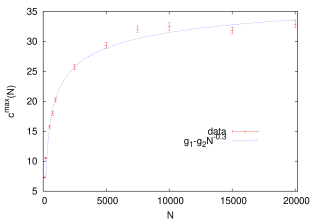
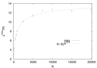
Figure 7: Data on the maximum of the average specific heat $\overline{c(T,N)}^{max}$ and on the maximum of the average susceptibility $\overline{\chi(T,N)}^{max}$, plotted as functions of chain lengths, together with the best fits to the law $g_{1}-g_{2}N^{e}$ with $g_{1},g_{2}>0$.

Figure 8: Evaluations of the finite size critical exponent $c_{r}(N)$, plotted as function of $1/N$. The results are from the fits of the probability distribution of the loop length to the expected law (36) $\overline{P^{*}_{\epsilon}(l,T_{c}(N),N)}\propto l^{c_{p}-c_{r}}$ (with $c_{p}=2.15$ and $T_{c}(N)$ taken as the temperature for which the average specific heat is maximum). For each chain length, data are fitted in the $l$-range (with $l>2$) in which $\overline{P^{*}(l,T_{c}(N),N)}$ is increasing with $l$. Here the errors are only indicative, as they depend strongly on the number of points in the range of the fit.

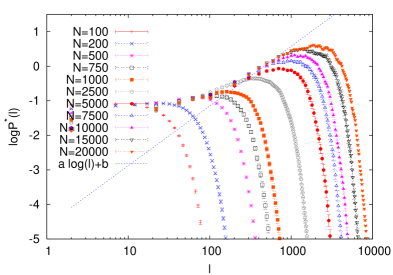
Figure 9: For the different chain lengths considered, data for $\overline{\log P^{*}_{\epsilon}(l,T_{c}(N),N)}$, at temperatures $T_{c}(N)$ for which average specific heats reach their maxima. The expected asymptotic behavior $(2.15-c_{r})\log l+b$ with $c_{r}=1.4$ (i.e. $c_{r}\sim 1+1/\nu_{r}$ with $\nu_{r}$ obtained from the fit of the maximum of the specific heat) is also plotted.

For further validation of this result, and for a better understanding of finite size corrections to scaling, we consider the fits of $\overline{P^{*}_{\epsilon}(l,T_{c}(N),N)}$ to the expected behavior $\propto l^{c_{p}-c_{r}}$ (36). We get correspondingly the size-dependent estimations of the critical exponent $c_{r}(N)$, which are presented in [Fig. 8]. Here the (finite size) critical temperatures $T_{c}(N)$ are taken as the temperatures for which the average specific heat reaches its maximum and we disregard the possible presence of a finite correlation length. We fit data by considering only the $l$-range (with $l>2$) in which $\overline{P^{*}_{\epsilon}(l,T_{c}(N),N)}$ is an increasing function of $l$ (see [Fig. 6]). The obtained values of $c_{r}(N)$, and therefore of $1/\nu_{r}(N)=\min\{1,c_{r}(N)-1\}$, for different chain lengths are definitely not compatible within the (though indicative) errors and one observes a clear trend towards decreasing $c_{r}(N)$ values for larger chain lengths. It is in particular interesting to notice that, for $N=200$, we still have $c_{r}(N)\simeq 2.1$ and correspondingly $\nu_{r}(N)=1$, whereas for $N\sim 1000$, we obtain $c_{r}(N)\sim 1.8\div 1.9$, again in perfect agreement with the results of [31] concerning the $3d$ DSAW-DNA on-lattice model. On the other hand, with the study of larger chain lengths it becomes clear that the transition is at least of second order with $\nu_{r}\geq 2$. In fact, for the largest size considered $N=20000$, the exponent obtained is $c_{r}(N)\simeq 1.5$. This implies that the correct evaluation of the (asymptotic) critical exponents, apart from finite size corrections, as $c_{r}=\lim_{N\rightarrow\infty}c_{r}(N)$ leads to $c_{r}\leq 1.5$. This value can be compatible with $c_{r}=1+1/\nu_{r}\sim 1.35$ obtained from the maximum of the specific heat.

It is nevertheless important to stress that the above results concern average quantities. The thermodynamic limit behavior of the typical sample could be therefore blurred by the fluctuations of the sequence-dependent pseudo-critical temperature, if they are governed by an exponent $\nu_{r,2}>\nu_{r,1}$ as suggested in [29, 30, 38, 39]. It is possible that we are only looking at the average correlation length $\xi_{2}(T,N)$, and in particular the value $c_{r}=1.5$ would be in agreement with the result $\nu_{r,2}=2$ in [30].

Accordingly, we consider also data on $\overline{\log P^{*}_{\epsilon}(l,T_{c}(N),N)}$, evaluated by averaging over disorder after taking the logarithm. To be precise, following [30], the quantity expected to be described by the typical correlation length $\xi_{1}$ is $\sum_{i}\log\{[Z^{f}_{\epsilon}(i,N)Z^{b}_{\epsilon}(i+l,N)]/Z^{*}_{\epsilon,N}\}$. Here we are instead considering a kind of mixed average, but the behavior of $\overline{\log P^{*}_{\epsilon}(l,T_{c}(N),N)}$ should anyway display differences with that of $\log\overline{P^{*}(l,T,N)}$ in the presence of two distinguishable correlation lengths. On the contrary, the comparison between [Fig. 9] and [Fig. 6] shows that, at least for $T=T_{c}(N)$, $\log{\overline{P_{\epsilon}}}$ and $\overline{\log{P_{\epsilon}}}$ behave similarly. In particular, $\overline{\log{P^{*}_{\epsilon}}}$ is also an increasing function of $l$ for the largest considered sizes, and on quantitative grounds the evaluated $c_{r}(N)$ values are essentially compatible within errors. In order to emphasize this point, the expected asymptotic behavior $\overline{\log{P^{*}_{\epsilon}}}\sim(2.15-c_{r})\log l+b$ with $c_{r}=1+1/\nu_{r}\sim 1.35$ (obtained from the average specific heat) is also plotted in [Fig. 9]. More quantitative analysis of these results are left for a forthcoming work [40].

5 Conclusions

We studied numerically a disordered PS model for DNA denaturation with $c_{p}=2.15$, which displays a first order transition in the homogeneous case, by solving recursively the equations for the canonical partition function with the SIMEX scheme. The model is made as similar as possible to the $3d$ DSAW-DNA previously studied by Monte Carlo like simulations [31] and it is expected that the results of the study could also be relevant to different disordered PS models with $c_{p}>2$.

We introduced the parameter $x=R/[\log\mu(R-1)]$, where $R=\epsilon_{GC}/\epsilon_{AT}$ is the ratio of the Guanine-Cytosine to the Adenine-Thymine coupling energies and $\mu$ is the connectivity constant of the corresponding on-lattice model. We showed that this parameter, at fixed $c_{p}$ value and GC composition (taken to be 1/2), appears to play the role of (the logarithm of) an intrinsic length scale, and to describe, in a first approximation, the finite size behavior. In particular, for a given $N$-value, the manifestation of the effect of disorder appears to be the most evident for the smallest $x$ values, in agreement with a qualitative explanation based on the possible occurrence of large enough rare regions. It is interesting to notice that, within this picture, the system size necessary for observing the asymptotic behavior and making evident the effect of disorder diverges exponentially with $x$.

We studied in detail the value $x=1.3$, obtained with $R=2$ and $\log\mu=1.54$ (as in [31]), for sequence sizes up to $N=20000$ (larger than the sizes accessible to Monte Carlo like simulations by a factor 20). We found that the model exhibits strong corrections to scaling, displaying a crossing between a still nearly pure system like behavior for small chain lengths $N\lesssim 1000$ and the observed (apparently asymptotic) large one for $N\gtrsim 5000$. In particular, the maximum of the average specific heat, which behaves as the susceptibility, increases with $N$ for small chain lengths. Considering the whole size range, it appears instead to be clearly saturating. This result shows that, at least from the point of view of average quantities, the thermodynamic limit is described by a random fixed point with $\alpha_{r}\leq 0$ and correspondingly $\nu_{r}\geq 2/d=2$. By fitting data with a scaling law of the form $g_{1}-g_{2}N^{\alpha_{r}/\nu_{r}}$, and by taking into account corrections to scaling, we find in particular $\alpha_{r}/\nu_{r}=-0.3\pm 0.1$, which by using the hyperscaling relation gives $\nu_{r}\sim 3$.

The average loop length probability distribution at the critical temperature appears still described by a power law at least on an interval $1\ll l\ll N$ of the range. Upon fitting data according to $\overline{P_{\epsilon}(l,T_{c}(N),N)}\propto 1/l^{c_{r}}$ one finds $N$-dependent values for the exponent which is compatible with $c_{p}$ for the smallest sizes whereas when looking at the whole $N$ range it appear to converge towards an asymptotic limit $c_{r}\leq 1.5$ (possibly compatible with $c_{r}=1+1/\nu_{r}\sim 1.35$). Moreover, $\overline{\log P(l,T_{c}(N),N)}$ exhibits also a similar behavior, suggesting that there is no difference between typical and average correlation lengths.

Our best-fit estimation, $\nu_{r}\sim 3$, is close to the estimation in [30] for the case $c_{p}=1.75$. This observation would support the hypothesis that disorder is relevant as soon as $c_{p}>3/2$ and that the various disordered PS models considered could be described by the same random fixed point corresponding to a transition which is at least of second order (and probably smoother), in agreement with recent analytical findings [32, 33, 34]. Our statistics do not allow nevertheless to completely rule out the possibility that $\nu_{r}=2$, particularly from $\overline{P_{\epsilon}}$ data, and in any event an analysis in terms of pseudo-critical temperatures [52, 29, 30, 54, 38, 39] is in order for clarifying the situation. We leave this development to a forthcoming work [40].

It is also interesting to notice that there are very recent theoretical studies [58, 59, 60] on the loop dynamics in PS models, which in particular relates the equilibrium loop length distribution probability to the correlation function, therefore suggesting a new intriguing method for measuring experimentally the $c$ value. From this point of view, the expected behavior of $P(l)$ in presence of disorder and the possibility of observing differences between the average and the typical sequence cases seems to us important questions to be clarified.

In conclusion, our results provide numerical evidence for strong finite size corrections to the asymptotic behavior of the disordered PS model considered. The data show moreover that disorder is relevant, at least from the analysis of average quantities. The findings here appear also to confirm that the evaluation $\nu_{r}\simeq 1.2$ in previous numerical study concerning on-lattice $3d$ DSAW-DNA model [31] is to be considered as lower bound for the correct (average) correlation length exponent. The observed behavior is in agreement with a proposed qualitative picture for finite size effects, which could also explain the difference with the results of previous studies on a different disordered PS model with the same $c_{p}$ [29, 30]. A preliminary presentation for part of the findings and hypotheses here can be found in [61].

Appendix

We use in the numerical computations the SIMEX implementation of the FF scheme [4, 5, 23], which relies on the numerical approximation of the powers $1/l^{c_{p}}$ by sums of exponentials:

$$\frac{1}{(2l)^{c_{p}}}\simeq\sum_{k=1}^{N_{S}}a_{k}\exp(-2lb_{k}).$$ (37)

In the present study we consider $c_{p}=2.15$ and the values for the coefficients $a_{k}$ and $b_{k}$, with $N_{S}=15$, provided in [29]. The computation of the recursive equations for the forward and backward partition functions were implemented with the introduction of free energy like quantities, in order to handle logarithms of $Z^{f}_{\epsilon}$ and $Z^{b}_{\epsilon}$ (following [24]).

In detail, the equation (18) for the forward partition function becomes:

$$Z^{f}_{\epsilon}(\rho+1)=\exp({\beta\epsilon_{\rho+1}-\log\mu})\left\{Z^{f}_{\epsilon}(\rho)+\sum_{k=1}^{N_{FF}}a_{k}\sum_{\rho^{\prime}=1}^{\rho-1}{Z^{f}_{\epsilon}(\rho^{\prime})}\exp[-2(\rho-\rho^{\prime}+1)b_{k}]\right\}.$$ (38)

By defining

$$Q_{k}(\rho)=\sum_{\rho^{\prime}=1}^{\rho}Z^{f}_{\epsilon}(\rho^{\prime})\exp(2\rho^{\prime}b_{k})=\exp[2\rho b_{k}+\mu_{k}(\rho)],$$ (39)

one obtains

$$Z^{f}_{\epsilon}(\rho)=\exp[\mu_{k}(\rho)]-\exp[\mu_{k}(\rho-1)-2b_{k}]$$ (40)

and a recursion relation for $\mu_{k}(\rho)$:

$$\mu_{k}(\rho+1) = \mu_{k}(\rho)+\log(A_{f}+B_{f}+C_{f})$$ (41)

$$A_{f} = \exp(-2b_{k})$$

$$B_{f} = \exp(\beta\epsilon_{\rho+1}-\log\mu)\left\{1-\exp[-2b_{k}+\mu_{k}(\rho-1)-\mu_{k}(\rho)]\right\}$$

$$C_{f} = \exp(\beta\epsilon_{\rho+1}-\log\mu)\left\{\sum_{j=1}^{N_{FF}}a_{j}\exp[-4b_{j}+\mu_{j}(\rho-1)-\mu_{k}(\rho)]\right\}$$

Analogously, one writes the equation for the backward partition function:

$$Z^{b}_{\epsilon}(\rho-1)=\exp({\beta\epsilon_{\rho-1}-\log\mu})\left\{Z^{b}_{\epsilon}(\rho)+\sum_{k=1}^{N_{FF}}a_{k}\sum_{\rho^{\prime}=\rho+1}^{N}{Z^{b}_{\epsilon}(\rho^{\prime})}\exp[-2(\rho^{\prime}-\rho+1)b_{k}]+1\right\},$$ (42)

and defines

$$R_{k}(\rho)=\sum_{\rho^{\prime}=\rho}^{N}Z^{b}_{\epsilon}(\rho^{\prime})\exp(-2\rho^{\prime}b_{k})=\exp[-2\rho b_{k}+\nu_{k}(\rho)],$$ (43)

obtaining

$$\nu_{k}(\rho-1) = \nu_{k}(\rho)+\log(A_{b}+B_{b}+C_{b}+D_{b})$$ (44)

$$A_{b} = \exp(-2b_{k})$$

$$B_{b} = \exp(\beta\epsilon_{\rho-1}-\log\mu)\left\{1-\exp[-2b_{k}+\nu_{k}(\rho+1)-\nu_{k}(\rho)]\right\}$$

$$C_{b} = \exp(\beta\epsilon_{\rho-1}-\log\mu)\left\{\sum_{j=1}^{N_{FF}}a_{j}\exp[-4b_{j}+\nu_{j}(\rho+1)-\nu_{k}(\rho)]\right\}$$

$$D_{b} = \exp(\beta\epsilon_{\rho-1}-\log\mu)\exp[-\nu_{k}(\rho)].$$

We used the boundary conditions (with the implicit assumption $Z^{f}_{\epsilon}(0)=Z^{b}_{\epsilon}(N+1)=0$):

$$Z^{f}_{\epsilon}(1) = \exp(\beta\epsilon_{1}-\log\mu)$$

$$Z^{f}_{\epsilon}(2) = \exp(\beta\epsilon_{1}-\log\mu)\exp(\beta\epsilon_{2}-\log\mu)$$

$$Z^{b}_{\epsilon}(N-1) = \exp(\beta\epsilon_{N-1}-\log\mu)[\exp(\beta\epsilon_{N}-\log\mu)+1]$$

$$Z^{b}_{\epsilon}(N) = \exp(\beta\epsilon_{N}-\log\mu),$$ (45)

and correspondingly:

$$\mu_{k}(1) = \beta\epsilon_{1}-\log\mu$$

$$\mu_{k}(2) = \beta\epsilon_{1}-\log\mu+\log[\exp(-2b_{k})+\exp(\beta\epsilon_{2}-\log\mu)]$$

$$\nu_{k}(N-1) = \beta\epsilon_{N}-\log\mu+\log\left\{\exp(-2b_{k})+\exp(\beta\epsilon_{N-1}-\log\mu)[1+\exp(-\beta\epsilon_{N}+\log\mu)]\right\}$$

$$\nu_{k}(N) = \beta\epsilon_{N}-\log\mu.$$ (46)

References

- [1] R. M. Wartell and A. S. Benight, Phys. Rep. 126, 67 (1985).
- [2] D. Poland and H.A. Scheraga (eds.), Theory of Helix-Coil Transitions in Biopolymers, (Academic, New York, 1970).
- [3] For a recent review in which the effects of self-avoidance in Poland-Scheraga models are critically discussed see C. Richard and A. J. Guttman, J. Stat. Phys. 115, 943 (2004).
- [4] M. Fixman and J.J. Freire, Biopolymers 16, 2693 (1977).
- [5] E. Yeramian, F. Schaeffer, B. Caudron, P. Claverie and H. Buc, Biopolymers 30, 481 (1990).
- [6] D. Poland and H.A. Scheraga, J. Chem. Phys. 45, 1456, 1464 (1966).
- [7] M.E. Fisher, J. Chem Phys. 45, 1469 (1966).
- [8] S. Cocco and R. Monasson, Phys. Rev. Lett. 83,5178 (1999).
- [9] N. Theodarakopoulos, T. Dauxois and M. Peyrard, Phys. Rev. Lett. 85, 6 (2000) and references therein.
- [10] Y. Kafri, D. Mukamel and L. Peliti, Phys. Rev. Lett. 85, 4988 (2000).
- [11] A. Hanke and R. Metzler Phys. Rev. Lett. 90, 159801 (2003); Y. Kafri, D. Mukamel and L. Peliti, Phys. Rev. Lett. 90 159802 (2003).
- [12] Y. Kafri, D. Mukamel and L. Peliti, Eur. Phys. J. B 27, 135 (2002).
- [13] M.S. Causo, B. Coluzzi and P. Grassberger, Phys. Rev. E 62, 3958 (2000).
- [14] E. Carlon, E. Orlandini and A.L. Stella Phys. Rev. Lett. 88, 198101 (2002).
- [15] M. Baiesi, E. Carlon, Y. Kafri, D. Mukamel, E. Orlandini and A.L. Stella, Phys. Rev. E 67, 021911 (2003).
- [16] T. Garel, C. Monthus and H. Orland, Europhys. Lett. 55, 132 (2001); S. M. Bhattacharjee, Europhys. Lett. 57, 772 (2002); T. Garel, C. Monthus and H. Orland, Europhys. Lett. 57,774 (2002).
- [17] S. Buyukdagli and M. Joyeux, Phys. Rev. E 73, 051910 (2006).
- [18] M.E. Fisher, J. Stat. Phys. 34, 667 (1984).
- [19] P. Belohorec and B. Nickel, Accurate Universal and Two-parameter Model Results from a Monte-Carlo Renormalization Group Study, Preprint - University of Guelph (1997).
- [20] D. Poland, Biopolymers 13, 1859 (1974).
- [21] G. Steger, Nucleic Acids Res. 22, 2760 (1994).
- [22] R.D. Blake et al, Bioinformatics, 15, 370 (1999).
- [23] E. Yeramian, Europhys. Lett. 25, 49 (1994).
- [24] T. Garel and H. Orland, Biopolymers 75, 453 (2004).
- [25] E. Yeramian, Gene 255, 139 (2000); Gene 255, 151 (2000).
- [26] E. Yeramian, S. Bonnefoy and G. Langsley, Bioinfomatics 18, 190 (2002).
- [27] E. Yeramian and L. Jones, Nucl. Acid Res. 31, 3843 (2003).
- [28] E. Carlon, M.L. Malki and R. Blossey, Phys. Rev. Lett. 94, 178101 (2005).
- [29] T. Garel and C. Monthus, J. Stat. Mech., P06004 (2005).
- [30] C. Monthus and T. Garel, Eur. Phys. J. B 48, 393 (2005).
- [31] B. Coluzzi, Phys. Rev. E 73, 011911 (2006).
- [32] G. Giacomin and F.L. Toninelli, Commun. Math. Phys 266, 1 (2006).
- [33] G. Giacomin and F.L. Toninelli, Phys. Rev. Lett. 96, 060702 (2006).
- [34] F.L. Toninelli, Critical properties and finite-size estimates for the depinning transition of directed random polymers, cond-mat/0604453, J. Stat. Phys. (in press, published on-line).
- [35] A.B. Harris, J. Phys. C 7, 1671 (1974).
- [36] M. Aizenman and J. Wehr, Phys. Rev. Lett. 62, 2503 (1989); Phys. Rev. Lett. 64, 1311(E) (1990).
- [37] A.N. Berker, Physica A194, 72 (1993).
- [38] C. Monthus, Random walks and polymers in the presence of quenched disorder, cond-mat/0601332. Proceedings of the conference Mathematics and Physics, I.H.E.S., Paris (France), November 2005.
- [39] C. Monthus and T. Garel, Random polymers and delocalization transition, cond-mat/0605448. Proceedings of the conference Inhomogeneous Random Systems, I.H.P., Paris (France), January 2006.
- [40] B. Coluzzi and E. Yeramian, Numerical evidence for the relevance of disorder in a Poland-Scheraga model for DNA denaturation with self-avoidance: An analysis in terms of pseudo-critical temperatures, work in progress.
- [41] B. Duplantier, Phys. Rev. Lett. 57, 941 (1986); J. Stat. Phys. 54, 581 (1989).
- [42] L. Schäfer, Can Finite Size Effects in the Poland-Scheraga Model Explain Simulations of a Simple Model for DNA Denaturation?, cond-mat/0502668.
- [43] D. Cule and T. Hwa, Phys. Rev. Lett. 79, 2375 (1997).
- [44] D.K. Lubensky and D.R. Nelson, Phys. Rev. Lett. 85, 1575 (2000); Phys. Rev. E 65, 031917 (2002).
- [45] S. Ares and A. Sánchez, Disorder Universality: the case of DNA denaturation cond-mat/0511532.
- [46] L.-H. Tang and H. Chaté, Phys. Rev. Lett. 86, 830 (2001).
- [47] Y. Kafri and D. Mukamel, Phys. Rev. Lett. 91, 055502 (2003).
- [48] V. Ivanov, Y. Zeng and G. Zocchi, Phys. Rev. E 70, 051907 (2004); V. Ivanov, D. Piontkovski and G. Zocchi, Phys. Rev. E 71 041909 (2005).
- [49] J.T. Chayes, L. Chayes, D.S. Fisher and T. Spencer, Phys. Rev. Lett. 57, 2999 (1986).
- [50] A. Aharony, A.B. Harris and S. Wiseman, Phys. Rev. Lett 81, 252 (1998).
- [51] F. Pázmándi, R.T. Scalettar and G.T. Zimányi, Phys. Rev. Lett. 79, 5130 (1997).
- [52] S. Wiseman and E. Domany, Phys. Rev. E 52, 3469 (1995); Phys. Rev. Lett. 81, 22 (1998); Phys. Rev. E 58, 2938 (1998).
- [53] T. Garel and C. Monthus, Eur. Phys. J. B 46, 117 (2005).
- [54] C. Monthus and T. Garel, J. Stat. Mech., P12011 (2005).
- [55] R. Blossey and E. Carlon, Phys. Rev. E 68, 061911 (2003).
- [56] E. Yeramian and P. Claverie, Nature 326, 169 (1987).
- [57] Z. Bay, Phys. Rev. 77, 419 (1950); P. Wahl and H. Lami, Biochem. Biophys. Acta 133, 233 (1967); I. Isenberg and R.D. Dyson, Biophys. J. 9, 1337 (1969).
- [58] A. Bar, Y. Kafri and D. Mukamel, Loop dynamics in DNA denaturation, cond-mat/0608663.
- [59] T. Ambjörnsson, S.K. Banik, M.A. Lomholt and R. Metzler, Master equation approach to DNA-brathing in heteropolymer DNA, cond-mat/0610547.
- [60] T. Novotný, J.N. Pedersen, T. Ambjörnsson, M.S. Hansen and R. Metzler, Bubble coalescence in breathing DNA: Two vicious walkers in opposite potentials, cond-mat/0610752.
- [61] B. Coluzzi and E. Yeramian, On the disordered SAW model for DNA denaturation, proceedings of the X International Workshop on Disordered Systems, Andalo (Italy), 18-21 March 2006. Philosophical Magazine (in press, published on-line).