Fluid-fluid demixing transitions
in colloid–polyelectrolyte star mixtures

Abstract

We derive effective interaction potentials between hard, spherical colloidal particles and star-branched polyelectrolytes of various functionalities $f$ and smaller size than the colloids. The effective interactions are based on a Derjaguin-like approximation, which is based on previously derived potentials acting between polyelectrolyte stars and planar walls. On the basis of these interactions we subsequently calculate the demixing binodals of the binary colloid–polyelectrolyte star mixture, employing standard tools from liquid-state theory. We find that the mixture is indeed unstable at moderately high overall concentrations. The system becomes more unstable with respect to demixing as the star functionality and the size ratio grow.

1 Introduction

Polyelectrolyte stars (PE’s) are complex macromolecules that have attracted a lot of interest in the recent past. They consist of $f$ polymer chains, all attached on a common centre, and carrying ionizable groups along their backbones. Solution of these molecules in a polar solvent results into dissociation of the groups, so that the chains turn into polyelectrolytes and stretch considerably with respect to their neutral conformations. Already in the early 1990s, the importance of the stretched PE-chains in stabilizing colloidal suspensions has been pointed out and analysed theoretically by Pincus [1] employing scaling theory as well as, more recently, by Wang and Denton [2] using linear-response theory. A distinguishing feature of PE-stars is their ability to adsorb the vast majority of the released counterions into their interior, creating thereby an inhomogeneous cloud of entropically trapped particles that provides a strong entropic barrier against coagulation [1, 2, 3, 4, 5, 6, 7, 8, 9]. The development of accurate effective interactions between the PE-stars [6, 7, 8, 9] has led to predictions regarding their overall phase behaviour with emphasis on crystallization [10, 11], which has recently received experimental corroboration [12].

Though a great deal has thus been learned regarding the behaviour of one-component solutions of PE-stars, the question of the influence of these ultrasoft colloids on solutions of hard colloids has not been investigated thus far. At the same time, the behaviour of PE-stars in the vicinity of planar or curved hard surfaces (such as a larger colloidal particle) is an issue of considerable interest, due to the possibility of manipulating the conformation of the PE-star by suitably changing the surface’s geometry or physical characteristics [13, 14, 15]. Recently, the properties of PE-stars close to hard, planar walls were investigated in detail by means of computer simulations and theory [16]. It has been found that the geometrical constraint of the planar wall does not affect the ability of the PE-stars to absorb the vast majority of their counterions. In addition, a new mechanism giving rise to a wall-star repulsion has been discovered, which rests on compression of stiff star chains against the neighboring wall. In this work, we proceed to the full, many body problem of a collection of PE-stars and neutral colloids, which can be seen as curved walls. Basing on the results of Ref. [16], we investigate the structure of the mixture and find that it is unstable against demixing as the concentration becomes sufficiently high. This work serves, thereby, as the reference point for future investigations on the effects of adding charge to the colloidal particles. It is specular to recently published work on mixtures of charged colloids with uncharged polymers [17], since in our case the colloids are neutral and the (star-branched) polymers are charged.

The rest of this paper is organised as follows: in sec. 2 we introduce the colloid–colloid and PE-star–PE-star effective interactions and we derive the cross interaction, based on previous results on the PE-star interaction potential with a planar wall. In sec. 3 we present our method for calculating structure and thermodynamics by employing the aforementioned interactions in combination with two-component liquid integral equation theories. In sec. 4 we present our results for various regimes of the parameter space as well as the overall phase diagrams of the mixture. Finally, in sec. 5 we summarize and draw our conclusions.

2 Effective pair potentials

The system under investigation is a binary colloid–PE-star mixture. The colloids are coded with the subscript ‘c’ and the PE-stars with ‘s’. The mixture contains, thus, $N_{\rm c}$ spherical, neutral colloids with diameter $\sigma_{\rm c}$ (radius $R_{\rm c})$ and $N_{\rm s}$ PE-stars in aqueous solution. The stars can be characterised by their degree of polymerization $N_{\rm p}$, functionality $f$, and charging fraction $\alpha$. Thereby, the $f$ chains of each star are charged in a periodical manner in such a way that every ($1/\alpha$)-th monomer carries a charge $e$. As a result, every star carries a total bare charge $Q=e\alpha fN_{\rm p}$, leaving behind $M=\alpha fN_{\rm p}$ monovalent, oppositely charged counterions in the mixture due to the requirement that the system must remain electro-neutral as a whole. With $\sigma_{\rm s}$ referring to the stars’ diameter, i.e., twice the average centre-to-end distance $R_{\rm s}$ of the arms, we define the size ratio $q$ between the two species as

$$q=\sigma_{\rm s}/\sigma_{\rm c}.$$ (1)

Within this work, we will only consider PE-stars that are smaller than the colloids, hence $q<1$. The degree of polymerization of every arm, $N_{\rm p}$, and the charging ratio $\alpha$ play a crucial role because they determine the number of released counterions $M$ mentioned above. The latter are, in turn, mainly responsible for the emergence of the star-star [1, 7, 8] and the star-colloid effective repulsions [16], due to the loss of entropy they experience when two such objects approach close to each other, see also eq. (3) in what follows. In this work, we fix $N_{\rm p}=50$ and $\alpha=1/3$ throughout. Generalizations to other values of $\alpha$ and $N_{\rm p}$ can follow by appropriately taking into account the dependence of $M$ on these parameters. Thereby, the two remaining single-molecule parameters that we vary are the stars’ functionality $f$ and the size ratio $q$.

The thermodynamic parameters are the partial number densities $\rho_{i}=N_{i}/V$ ($i={\rm c},{\rm s}$) of the respective species and the absolute temperature $T$. Alternatively, we can work with the concentrations $x_{i}=N_{i}/N$ and the total number density $\rho=N/V$, with the total particle number $N=N_{\rm c}+N_{\rm s}$ in the overall volume $V$ of our model system. We will consider constant, room temperature ($T=300\,{\rm K}$) throughout this work. This is the temperature for which the star-star effective interactions [7, 8] and the PE-star–planar wall potentials [16] have been derived, based on the value $\lambda_{\rm B}=7.1\,{\rm\AA}$ for the Bjerrum length in aqueous solvents. As usual, we define the inverse thermal energy $\beta=1/(k_{\rm B}T)$, with $k_{\rm B}$ denoting Boltzmann’s constant.

The starting point for all considerations to follow are the effective pair potentials between the constituent mesoscopic particles, having integrated out all the monomer, solvent and counterions degrees of freedom. When introducing this set of interactions as an input quantity into the full two-component integral equation theory described in more detail in Sec. 3, we can in principle completely access the structure and thermodynamics of the system at hand.

2.1 The colloid–colloid and PE-star–PE-star interactions

The effective colloid–colloid interaction at centre-to-centre distance $r$ is simply taken to be a pure hard sphere (HS) potential, namely:

$$\beta V_{\rm cc}(r)=\left\{\begin{array}[]{ll}\infty&r\leq\sigma_{\rm c};\\ 0&{\rm else}.\end{array}\right.$$ (2)

A lot of work concerning effective PE-star–PE-star interactions was done in the recent past by Jusufi and co-workers [7, 8]. They employed monomer-resolved Molecular Dynamics (MD) simulations and analytical theories and found an ultra-soft, bounded, density-dependent effective interaction governed by the entropic repulsions of counterions trapped in the interior of the stars. The good agreement between simulations and theory even allowed them to put forward analytic expressions for the full pair potential at arbitrary star separations. The effective potential has a weak density-dependence, which however disappears when the star density exceeds its overlap value $\rho_{\rm s}^{*}$. In this case, all counterions are absorbed within the stars, whose bare charges are therefore completely compensated. Thus, the effective potential vanishes identically for centre-to-centre distances $r>\sigma_{\rm s}$. For overlapping distances $r\leq\sigma_{\rm s}$, there is no dependence on the concentration anymore and only the trapped counterions’ entropy contributes to the star–star interaction, for this reason reading for $r\leq\sigma_{\rm s}\equiv q\sigma_{\rm c}$ as [7, 8, 10, 11]:

$$\frac{\beta V_{\rm ss}(r)}{2N_{2}}=\ln\left\{\frac{N_{2}}{2\pi\left[1+\frac{r}{q\sigma_{\rm c}}\left(1-\ln\left(\frac{r}{q\sigma_{\rm c}}\right)\right)\right]}\right\}+\frac{\frac{r}{q\sigma_{\rm c}}\ln^{2}\left(\frac{r}{q\sigma_{\rm c}}\right)}{1+\frac{r}{q\sigma_{\rm c}}\left(1-\ln\left(\frac{r}{q\sigma_{\rm c}}\right)\right)}-\ln\left(\frac{N_{2}}{4\pi}\right).$$ (3)

In eq. (3) above, $N_{2}$ is the number of spherically trapped counterions of a single star. It does not coincide with the number of released counterions, $M$, because the number $N_{1}$ of Manning-condensed counterions [19] does not contribute to the effective interaction and must be excluded: thus $N_{2}=M-N_{1}$. Extensive simulations [7, 8, 16, 21] have shown that the relative population of counterions in the two possible states is essentially independent of $r$. Thus, we fix $N_{1}$ to the value measured in MD simulations made during the investigation of PE-stars in planar confinement [16]. The fraction $N_{1}/M$ typically grows with increasing $\alpha$ and covers ranges between $30\%$ and $50\%$.

Clearly, the interaction $V_{\rm ss}(r)$ of eq. (3) vanishes, along with its first derivative with respect to $r$, at $r=q\sigma_{\rm c}$, guaranteeing the smooth transition to the region $r>q\sigma_{\rm c}$, in which $V_{\rm ss}(r)=0$. The latter feature is, strictly speaking, valid only for star densities exceeding the overlap value $\rho_{\rm s}^{*}$ [11]. For $\rho_{\rm s}<\rho_{\rm s}^{*}$, a Yukawa tail exists, emerging from the Coulomb interaction between the non-neutralised PE-stars and screened by the free counterions. For the purposes of simplicity, we ignore this small contribution, because the number of released counterions from multiarm PE-stars constitutes, at all densities, a tiny fraction of the total number of counterions $M$ [8], as confirmed by the very small values of experimentally measured osmotic coefficients of PE-star solutions [18].

2.2 The cross interaction

In order to complete the set of effective pair potentials needed to describe the binary mixture within the framework of a full two-component picture, we have to specify the colloid–PE-star cross interaction. Thereby, we proceed along the lines of Ref. [22] to derive the desired potential for small $q$-values based on results for the effective repulsion in the case where a PE-star is brought within a distance $z$ from a hard, flat wall [16, 21].

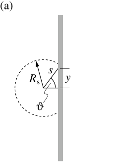
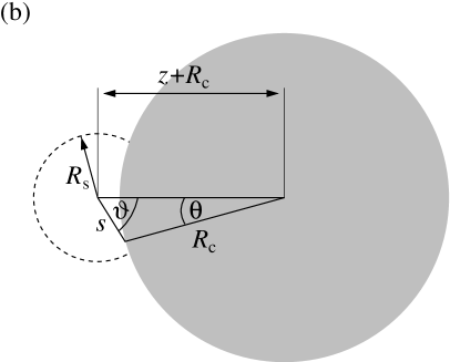
Figure 1: PE-star (smaller, dashed sphere) interacting with (a) a planar wall or (b) a hard colloidal particle (bigger, solid-gray sphere).

To begin with, let $V_{\rm sw}(z)$ be the star–wall interaction and $F_{\rm sw}(z)=-\partial V_{\rm sw}(z)/\partial z$ the corresponding force for a PE-star with all its counterions absorbed, i.e., for densities $\rho_{\rm s}$ beyond the overlap density (see also previous Sec. 2.1). Then, for the geometry shown in fig. 1(a), the force is related to the osmotic pressure $\Pi(s)$ exerted by the star on the surface of the wall via integration of the normal component of the latter along the area of contact [1]:

$$F_{\rm sw}(z)=2\pi\int_{0}^{\infty}{\rm d}y\,y\,\Pi(s)\cos\vartheta=2\pi z\int_{z}^{\infty}{\rm d}s\,\Pi(s).$$ (4)

Using the above eq. 4, we can directly obtain the functional form for the osmotic pressure $\Pi(z)$, provided that the functional form for the star–wall force $F_{\rm sw}(z)$ is known:

$$\Pi(z)=-\frac{1}{2\pi}\frac{\rm d}{{\rm d}z}\left(\frac{F_{\rm sw}(z)}{z}\right).$$ (5)

The same ideas can in principle be applied for a PE-star in the vicinity of a spherical, hard colloid, i.e., a hard sphere. Again, integrating the osmotic pressure along the area of contact between both objects yields the force acting on the centres of the mesoscopic particles. Pursuant to the geometry of the problem, see fig. 1(b), and paying regard to the underlying symmetry, we get as result for the colloid–PE-star cross force $F_{\rm cs}^{*}(z)$:

$$F_{\rm cs}^{*}(z)=\frac{\pi\sigma_{\rm c}^{2}}{2}\int_{0}^{\theta_{\rm max}}{\rm d}\theta\,\sin\theta\,\Pi(s)\cos\vartheta.$$ (6)

Here, the upper integration boundary $\theta_{\rm max}$ can be acquired by the condition that $\Pi(s)$ must vanish identically for all $\theta>\theta_{\rm max}$. It is possible to eliminate the polar angles $\vartheta$ and $\theta$ emanating from the centres of the PE-star and the colloid, respectively, in favor of the distance $s$ between the star centre and the point on the colloid’s surface that is determined by the aforementioned angles. In doing so, we use geometrical relations evident from the sketch in fig. 1(b), and finally obtain:

$$F_{\rm cs}^{*}(z)=\frac{\pi\sigma_{\rm c}}{2\left(\sigma_{\rm c}+2z\right)^{2}}\int_{z}^{s_{\rm max}}{{\rm d}s\,\left[\left(\sigma_{\rm c}+2z\right)^{2}-\sigma_{\rm c}^{2}+4s^{2}\right]\Pi(s)}.$$ (7)

Again, we may obtain the maximum integration distance $s_{\rm max}$ (without any need to calculate $\theta_{\rm max}$ before) simply by demanding that $\Pi(s)$ must be equal to zero for all $s>s_{\rm max}$. For such values of $s$, the integrand as a whole obviously vanishes and there are no contributions to the result of the integration anymore. Presumed the functional form for the osmotic pressure is known, such identification of $s_{\rm max}$ is rather easily feasible.

Since we want to consider small values $q\leq 0.3$ of the size ratio only, the stars discern the colloidal surface to be rather weakly bent compared to a flat wall, i.e., the radius of curvature is large in terms of the star diameter $\sigma_{\rm s}$. Therefore, it is a reasonable approximation to assume that the osmotic pressure remains almost unchanged with respect to the situation where a PE-star is brought in contact with a planar wall. Consequently, we may combine eqs. (5) and (7) to obtain a sound estimate for the effective force $F_{\rm cs}^{*}(z)$ as a function of distance of the star centre and the colloid’s surface. Note that in our special case $s_{\rm max}$ is of the order of the star radius $R_{\rm s}$. This fact becomes evident from eq. (5) if one takes into account that the typical range for the star–wall force $F_{\rm sw}(z)$ is also approximately $R_{\rm s}$ or at the utmost slightly bigger due to effects of a chain compression at the hard wall (see below) [16]. Clearly, the corresponding potential is received by a simple, one-dimensional integration:

$$V_{\rm cs}^{*}(z)=\int_{\infty}^{z}{\rm d}z^{\prime}\,F_{\rm cs}^{*}(z^{\prime}).$$ (8)

In fig. 2 we show the shape of $V_{\rm cs}^{*}(z)$ for $q=0.2$ and different values of the stars’ functionality $f$. In order to demonstrate the importance of the so-called compression term adding to the star–wall force $F_{\rm sw}$ besides electrostatic-entropic contributions [16], we additionally included colloid–star potentials calculated on the basis of the electrostatic and entropic star–wall forces alone. Since there are striking deviations, we can clearly expect such devolved compression effects to influence the phase behaviour of the mixture.

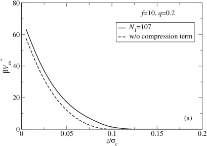
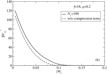
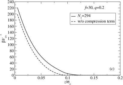
Figure 2: Effective colloid–PE-star potentials with and without provision for compression effects as a function of the centre-to-surface distance $z$. Here, we have chosen the parameters $q=0.2$ and (a) $f=10$, (b) $f=18$, and (c) $f=30$. In the legend boxes, the numbers of condensed counterions $N_{1}$ used as fit parameters in Ref. [16] are specified for sake of completeness.

Finally, we need to express the effective potential as a function of the particles’ centre-to-centre separation $r$ instead of the centre-to-surface distance $z$. Thereby, we have to take into account that the star centre is strictly forbidden to penetrate the volume of the colloid. Thus, the total cross interaction features a hard core plus the soft, purely repulsive tail as obtained from the above eq. (8) and finally writes as:

$$V_{\rm cs}(r)=\left\{\begin{array}[]{ll}\infty&r\leq\sigma_{\rm c}/2\\ V_{\rm cs}^{*}(r-\sigma_{\rm c}/2)&{\rm else}.\end{array}\right.$$ (9)

3 Determination of the structure and thermodynamics of the mixture

In this section, we describe the basic principles of liquid integral equation theory for binary mixtures and how to subsequently access the thermodynamics of the system. In general, the pair structure of the system at hand (and analogously any other two-component system) is fully described by three independent total correlation functions $h_{ij}(r)$ with $i,j={\rm c,s}$. Hereby, we already allowed for the symmetry with respect to exchange of the indices, i.e., $h_{ij}(r)=h_{ji}(r)$. Closely related to the total correlation functions are the so-called direct correlation functions (dcf’s) $c_{ij}(r)$. Following the same symmetry argument again, there exist only three independent dcf’s. In what follows, we will denote the Fourier transforms of $h_{ij}(r)$ and $c_{ij}(r)$ as $\tilde{h}_{ij}(r)$ and $\tilde{c}_{ij}(r)$, respectively.

The above-mentioned connection between the total and direct correlation functions is quantitatively incorporated via the multicomponent generalization of the well-known and commonly used Ornstein-Zernike (OZ) relation, which in its Fourier space representation reads as [23, 24, 25]:

$${\bf\tilde{H}}(k)={\bf\tilde{C}}(k)+{\bf\tilde{C}}(k)\cdot{\bf D}\cdot{\bf\tilde{H}}(k).$$ (10)

Here, ${\bf\tilde{H}}(k)$ and ${\bf\tilde{C}}(k)$ are symmetric $(2\times 2)$ matrices whose elements are constituted by the total and direct correlation functions, respectively, and ${\bf D}$ is a diagonal $(2\times 2)$ matrix containing the partial densities characterising the composition of the system under investigation, i.e.,

$$\left[{\bf\tilde{H}}(k)\right]_{ij}=\tilde{h}_{ij}(k),\;$$ (11)

$$\left[{\bf\tilde{C}}(k)\right]_{ij}=\tilde{c}_{ij}(k),$$ (12)

$$\left[{\bf D}\right]_{ij}=\rho_{i}\delta_{ij}.$$ (13)

Evidently, eq. (10) can be rewritten yielding the equivalent matrix relation

$${\bf\tilde{H}}(k)=\left[{\bf 1}-{\bf\tilde{C}}(k)\cdot{\bf D}\right]^{-1}\cdot{\bf\tilde{C}}(k),$$ (14)

with the identity matrix ${\bf 1}$ and the matrix inverse $\left[{\bf 1}-{\bf\tilde{C}}(k)\cdot{\bf D}\right]^{-1}$. Defining $\Delta(k)\equiv\rho_{\rm s}\rho_{\rm c}[\tilde{c}_{\rm ss}(k)\tilde{c}_{\rm cc}(k)-\tilde{c}_{\rm cs}^{2}(k)]$ and $E(k)\equiv\rho_{\rm s}\tilde{c}_{\rm ss}(k)+\rho_{\rm c}\tilde{c}_{\rm cc}(k)$ and returning to a component-by-component notation, the latter can consistently be expressed in the following fashion:

$$\tilde{h}_{ij}(k)=\frac{\tilde{c}_{ij}(k)-\rho_{i}^{-1}\cdot\Delta(k)\cdot\delta_{ij}}{1+\Delta(k)-E(k)}.$$ (15)

The linear algebraic system of eq. (15), provides three independent equations coupling six yet unknown functions $\tilde{h}_{ij}(k)$ and $\tilde{c}_{ij}(k)$. In order to completely determine that set of functions, we therefore need to supply three additional relations to close and subsequently solve the system of equations. There are several popular choices for these so-called closures, e.g., the Percus-Yevick (PY) or hypernetted-chain (HNC) approximations in their respective two-component generalizations. While the former is known to generate reliable results for short-range interactions, the latter furnishes very accurate estimates for the pair structure in case of long-ranged, soft potentials. Neither the PY nor the HNC closure are thermodynamically consistent, however, and in our case this is a crucial factor, since we are interested in the calculation of phase boundaries, which should not depend on the route chosen to calculate the free energies. Thus, we resort to the Rogers-Young (RY) closure [26], in which thermodynamic consistency can be enforced. In its multicomponent version the RY-closure reads as:

$$g_{ij}(r)=\exp\left[-\beta V_{ij}\right]\cdot\left\{1+\frac{\exp\left[\chi_{ij}(r)f_{ij}(r)\right]-1}{f_{ij}(r)}\right\},$$ (16)

where $g_{ij}(r)=h_{ij}(r)+1$ are the so-called radial distribution functions and we introduced new auxiliary functions $\chi_{ij}(r)=h_{ij}(r)-c_{ij}(r)$. $V_{ij}(r)$ refers to the pair interactions between species $i$ and $j$ as presented in sec. 2. It may be again emphasised that the main benefit we gain from using the modified relation (16) is closely related to the hybrid character of the latter. Due to the fact that any closure constitutes an approximation, we in general obtain different results for the partial and total isothermal compressibilities as calculated via either the virial or the fluctuation route (see below), as already mentioned above. But the three mixing functions emerging in eq. (16) above and given by

$$f_{ij}(r)=1-\exp\left[-\zeta_{ij}r\right],$$ (17)

with $\zeta_{ij}$ being the so-called self-consistency parameters, now allow us to address this problem and to appropriately match the isothermal compressibilities. Since it is sufficient to apply a single consistency condition only, namely the requirement of equality of the system’s total virial and fluctuation isothermal compressibilities, the usual approach is to employ just one individual parameter $\zeta_{ij}=\zeta$ for all components. Hence, only a single mixing function $f_{ij}(r)=f(r)$ remains. However, multi-parameter versions of the RY closure have nevertheless also been proposed some years ago [27], accordingly demanding the equality of all the partial compressibilities. It is easy to check that for $\zeta=0$ and $\zeta=\infty$ the multicomponent PY and HNC closures, respectively, are recovered from eq. (16).

Now, we have to address in more detail the issue of calculating the total isothermal compressibility following the different routes. At first, we concern ourselves with the virial compressibility $\kappa_{T}^{\rm v}$. The total pressure $P$ of the system at hand, including both ideal and excess contributions, takes the form [25]:

$$\beta P=\rho-\frac{2\pi\rho^{2}}{3}\sum_{i}\sum_{j}x_{i}x_{j}\int_{0}^{\infty}{\rm d}r\,r^{3}\,V_{ij}^{\prime}(r)\,g_{ij}(r),$$ (18)

with $V_{ij}^{\prime}(r)=-\partial V_{ij}(r)/\partial r$ being the different pair potentials’ derivatives with respect to the inter-particle distance $r$. Provided the pressure pursuant to eq. (18) is known, $\kappa_{T}^{\rm v}$ can be obtained by differentiating with respect to the total density $\rho$ while the partial concentrations $x_{i}$ are kept fixed:

$$\rho k_{\rm B}T\kappa_{T}^{\rm v}=\left[\left.\frac{\partial(\beta P)}{\partial\rho}\right|_{\{x_{i}\}}\right]^{-1}.$$ (19)

In order to evaluate the fluctuation compressibility $\kappa_{T}^{\rm fl}$, we initially introduce the three partial structure factors $S_{ij}(k)$. As the correlation functions and the radial distribution functions, respectively, they also describe the structure of the system:

$$S_{ij}(k)=\delta_{ij}+\sqrt{\rho_{i}\rho_{j}}\tilde{h}_{ij}(k).$$ (20)

While for the one-component case the compressibility can simply be obtained as the $(k=0)$-value of the static structure factor, i.e., $S(k=0)=\rho k_{\rm B}T\kappa_{T}^{\rm fl}$, things are a bit more complicated for binary (or multicomponent, $\nu>2$) mixtures. Here, in generalization of the one-component situation, the compressibility can finally be written using the following expression [28, 29, 30]:

$$\rho k_{\rm B}T\kappa_{T}^{\rm fl}=\frac{S_{\rm ss}(0)S_{\rm cc}(0)-S_{\rm cs}^{2}(0)}{x_{\rm c}S_{\rm ss}(0)+x_{\rm s}S_{\rm cc}(0)-2\sqrt{x_{\rm s}x_{\rm c}}S_{\rm cs}^{2}(0)}.$$ (21)

Based on the knowledge of the partial correlation functions $h_{ij}(r)$ and structure factors $S_{ij}(k)$ as obtained by (numerically) solving the OZ relation, eq. (10), and using the RY closure, eq. (16), we can in principle completely access the thermodynamics of the system at hand. In order to calculate the binodal lines, a very convenient quantity to consider is the concentration structure factor $S_{\rm con}(k)$. It is a linear combination of all the partial structure factors, whereby the corresponding pre-factors are determined by the different species’ concentrations $x_{i}$, namely:

$$S_{\rm con}(k)=x_{\rm c}x_{\rm s}^{2}S_{\rm cc}(k)+x_{\rm s}x_{\rm c}^{2}S_{\rm ss}(k)-2(x_{\rm c}x_{\rm s})^{3/2}S_{\rm cs}(k).$$ (22)

Now, let $P$ be the total pressure according to the above eq. (18) and $g(x_{\rm s},P,T)=G(x_{\rm s},N,P,T)/N$ the Gibbs free energy $G(x_{\rm s},N,P,T)$ per particle. Then, the second derivative of the former is connected to the concentration structure factor $S_{\rm con}(k)$ by means of the sum rule [31, 32, 33]:

$$\beta g^{\prime\prime}(x_{\rm s},P,T)\equiv\beta\frac{\partial^{2}g(x_{\rm s},P,T)}{\partial x_{\rm s}^{2}}=\frac{1}{S_{\rm con}(0;x_{\rm s})},$$ (23)

where we have added the concentration $x_{\rm s}$ as a second argument to $S_{\rm con}(k)$ to emphasise this dependence. This differential equation has to be integrated along an isobar for any prescribed value of the pressure $P^{*}\equiv\beta P\sigma_{\rm c}^{3}={\rm const}$, to obtain the Gibbs free energy from the structural data, $S_{\rm con}(k=0;x_{\rm s})$. A detailed analysis of the limiting behaviour of $g^{\prime\prime}(x_{\rm s})$ shows a divergence as $1/x_{\rm s}$ for $x_{\rm s}\rightarrow 0$ and as $1/(1-x_{\rm s})$ for $x_{\rm s}\rightarrow 1$ [33]. In order to avoid any technical difficulties when numerically integrating, we a priori split the Gibbs free energy $g(x_{\rm s})$ into a term that arises from its ideal part and a remainder, which we call excess part, $g_{\rm ex}(x_{\rm s})$:

$$\beta g(x_{\rm s}) = (1-x_{\rm s})\ln(1-x_{\rm s})+x_{\rm s}\ln(x_{\rm s})$$ (24)

$$+ 3(1-x_{\rm s})\ln(\Lambda_{\rm c}/\sigma_{\rm c})+3x_{\rm s}\ln(\Lambda_{\rm s}/\sigma_{\rm c})+\beta g_{\rm ex}(x_{\rm s}),$$

with the thermal de Broglie wavelengths $\Lambda_{\rm c,s}$ of the colloids and the stars, respectively. Taking the second derivative in the above eq. (24) again, we obtain:

$$\beta g^{\prime\prime}(x_{\rm s})=\frac{1}{x_{\rm s}}+\frac{1}{1-x_{\rm s}}+g_{\rm ex}^{\prime\prime}(x_{\rm s}).$$ (25)

Thus, the ideal part of the Gibbs free energy is exclusively responsible for the appearance of the aforementioned divergences at the integration boundaries and the modified second-order differential equation

$$\beta g_{\rm ex}^{\prime\prime}(x_{\rm s})=\frac{1}{S_{\rm con}(0;x_{\rm s})}-\left(\frac{1}{x_{\rm s}}+\frac{1}{1-x_{\rm s}}\right)$$ (26)

for the excess Gibbs free energy alone is obviously free of any diverging terms. We can therefore easily solve it numerically. Subsequent addition of the analytically known ideal term $g_{\rm id}(x_{\rm s})=(1-x_{\rm s})\ln(1-x_{\rm s})+x_{\rm s}\ln(x_{\rm s})$ directly yields the total Gibbs free energy per particle that we are interested in. The two terms involving the thermal de Broglie wavelength are linear in $x_{\rm s}$; they only provide a shifting of the chemical potentials and can be dropped.

Thermodynamic stability requires that $g(x_{\rm s})$ is convex [34]. In case we encounter some $x_{\rm s}$-region where $g^{\prime\prime}(x_{\rm s})<0$ the binary mixture features a fluid-fluid demixing transition. In that sense, eqs. (23) and (26), respectively, allow us to investigate the thermodynamics and the phase behaviour of the system at hand by providing a tool to compute the Gibbs free energy (per particle). The corresponding phase boundaries can be calculated using Maxwell’s common tangent construction, which guarantees that the chemical potentials, $\mu_{i}$, are the same between both coexisting phases. Since we are in a situation where we moreover fixed the pressure $P^{*}$ of the mixture and its absolute temperature $T$, all conditions for phase coexistence are clearly fulfilled. Concretely, the common tangent construction amounts to solving the coupled equations

$$g^{\prime}(x_{\rm s}^{\rm I})=g^{\prime}(x_{\rm s}^{\rm II})$$ (27)

and

$$g(x_{\rm s}^{\rm I})-x_{\rm s}^{\rm I}g^{\prime}(x_{\rm s}^{\rm I})=g(x_{\rm s}^{\rm{II}})-x_{\rm s}^{\rm{II}}g^{\prime}(x_{\rm s}^{\rm{II}})$$ (28)

for the concentrations $x_{\rm s}^{\rm{I,II}}$ of the coexisting phases I and II.

In integrating eq. (25) above and adding the ideal terms, one obtains the Gibbs free energy per particle, $g(x_{\rm s})$ modulo an undetermined linear function $C_{1}x_{\rm s}+C_{0}$ with the constants $C_{1}$ and $C_{0}$ to be fixed by appropriate boundary conditions. As is clear from eqs. (27) and (28) above, such a linear term is anyway immaterial from the determination of phase boundaries and, in practice, it can be ignored on the same grounds that the terms involving the thermal de Broglie wavelengths in eq. (24) have been dropped. Nevertheless, the constants $C_{1}$ and $C_{0}$ can be determined as follows. Taking into account that the Gibbs free energy $G(N,P,x_{\rm s},T)$ is an extensive function but in its natural argument list there is only one extensive variable, namely the number of particles $N$, Euler’s theorem [35] asserts the function $g$ to have the form:

$$g(x_{\rm s})=x_{\rm s}\mu_{\rm s}(x_{\rm s})+(1-x_{\rm s})\mu_{\rm c}(x_{\rm s}).$$ (29)

For both limiting one-component cases, i.e., if no stars ($x_{\rm s}=0$) or no colloids ($x_{\rm s}=1$) are present in the system, the following relation holds true:

$$\beta g=\hat{f}+\rho\hat{f}^{\prime}=\ln(\rho)+\hat{f}_{\rm ex}+\rho\hat{f}^{\prime}_{\rm ex},$$ (30)

where $\hat{f}=\beta F/N$ denotes the Helmholtz free energy per particle and $\hat{f}^{\prime}$ its derivative with respect to the density $\rho$; the subscript ‘ex’ refers to the excess part of $\hat{f}$. On the other hand, $\hat{f}_{\rm ex}^{\prime}$ is connected to the excess pressure $P_{\rm ex}$ [as known from eq. (18) above] via the equation

$$\hat{f}^{\prime}_{\rm ex}=\beta P_{\rm ex}/\rho^{2}.$$ (31)

Following eq. (31), $\hat{f}^{\prime}_{\rm ex}$ can be obtained by integrating the ratio $P_{\rm ex}/\rho^{2}$ with respect to $\rho$ and applying the additional boundary condition $\hat{f}_{\rm ex}(\rho\rightarrow 0)=0$. Once the Helmholtz free energies for the pure colloid and PE-star systems are known this way, the corresponding chemical potentials $\mu_{\rm c}(0)$ and $\mu_{\rm s}(1)$ can be calculated and the conditions $g(0)=\mu_{\rm c}(0)$ and $g(1)=\mu_{\rm s}(1)$ for any arbitrary pressure $P$ [cf. eqs. (29) and (30) above], yield $C_{0}$ and $C_{1}$. Note that for the pure colloidal system, $x_{\rm s}=0$, we can avoid the integration route to compute the pressure, by using the accurate Carnahan-Starling expressions for hard-spheres [36], which also turn out to be consistent with the one calculated from the Rogers-Young route, based on eq. (18) and our results for the radial distribution function $g(r)$.

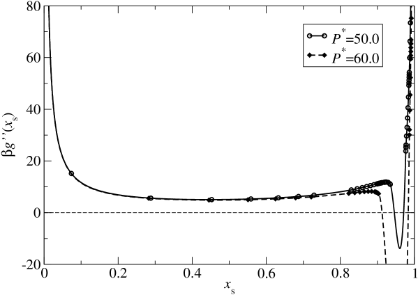
Figure 3: Examples of the second derivative of the Gibbs free energy per particle, $g^{\prime\prime}(x_{\rm s})$, plotted against the star concentration $x_{\rm s}$ for stars with functionality $f=30$, PE-star–colloid size ratio $q=0.2$, and two different pressures $P^{*}=\beta P\sigma^{3}_{\rm c}$. Symbols are calculated from the OZ relation, lines were obtained by cubic spline interpolation. Note that the $x_{\rm s}$-interval where we are not able to numerically solve the integral equations grows distinctly upon increasing the pressure, i.e., as we move away from the critical point. Moreover, the plot illustrates the limiting behaviour of $g^{\prime\prime}(x_{\rm s})$ as $1/x_{\rm s}$ for $x_{\rm s}\rightarrow 0$ and as $1/(1-x_{\rm s})$ for the opposite case $x_{\rm s}\rightarrow 1$, respectively.

Note that, when crossing the spinodal line in the density plane, the long wavelength limits of the partial structure factors, $S_{ij}(k\rightarrow 0)$, take non-physical values. This behaviour expresses the system’s physical instability against a possible fluid-fluid phase separation. Thereto, it is not feasible to (numerically) solve the integral equations anymore once we reached the spinodal; in fact, integral equation theories themselves break down before the spinodal is reached, yet after the binodal [37]. Consequently, depending on the total pressure and above a certain threshold value of the same, $P>P_{\rm thr}$, the concentration structure factor $S_{\rm con}(0;x_{\rm s})$ is unknown over some interval $\Delta x_{\rm s}(P)$. Hence, we need to appropriately interpolate $S_{\rm con}(0;x_{\rm s})$ in order to obtain the second derivative of the Gibbs free energy per particle for all $0\leq x_{\rm s}\leq 1$ and, in this way, to allow for the integration of the differential equations (23) or (26), respectively. Along the lines of Ref. [33], we perform this necessary interpolation using cubic splines. In order to illustrate the whole procedure, fig. 3 shows the function $g^{\prime\prime}(x_{\rm s})$ as computed from the OZ equation together with its cubic spline interpolation for a representative parameter combination and two different pressures. Moreover, in fig. 4, we plotted the corresponding Gibbs free energy $g(x_{\rm s})$ for the lower one of these pressures. In addition, the inset depicts Maxwell’s common tangent construction used to compute the star concentrations for the coexisting phases.

It may be emphasised that the results for the binodal do not depend on the concrete interpolation scheme, at least as long as the numerical methods used to solve the OZ relation are able to precisely reach the spinodal, i.e., the points where the structure factors diverge for $k\rightarrow 0$. Admittedly, this is not always strictly the case since the numerical schemes we employed to calculate correlation functions and corresponding structure factors, respectively, may break down slightly before the spinodal is reached. Accordingly, small inaccuracies induced by the interpolation procedure arise which grow with increasing width of the gap region $\Delta x_{\rm s}(P)$, or to put it in other words, with increasing pressure $P$, i.e., if we move away from the critical point. As long as the aforementioned interval where no solution of the integral equations can be found is rather small, we expect the interpolation to be reliable, while for higher pressures the received binodals are of more approximate character. Nevertheless, they still show a very reasonable behaviour. We are going to discuss the results for the phase diagrams in detail in sec. 4.3.

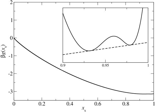
Figure 4: Gibbs free energy per particle $g(x_{\rm s})$ vs. the star concentration $x_{\rm s}$, plotted for $f=30$, $q=0.2$, and $P^{*}=50.0$. The curve was obtained via integrating the interpolated function $g^{\prime\prime}(x_{\rm s})$ twice according to the procedure delineated in the main text, whereby we subtracted an arbitrary linear function afterwards. The inset shows $g(x_{\rm s})$ with an differently scaled $x_{\rm s}$-axis in order to highlight the concave parts of the function and to show Maxwell’s common tangent construction.

4 Results

4.1 Low colloid-density limit

Based on the radial distribution functions $g(r)$ as obtained by the OZ relation closed with the RY closure, eqs. (10) and (16), we may map our two-component mixture onto an effective one-component system of the colloids alone. In doing so, the PE-stars are completely traced out, resulting into an effective colloid–colloid interaction where the pure hard-sphere potential is masked by additional depletion contributions originating in the presence of the stars and the forces they exert on the colloids. To put it in other words, the colloid–PE-star interactions cause spatial correlations of the PE-star distribution in the vicinity of the colloids, and it is exactly these correlations that determine the resulting shape of the depletion potential. Note that the latter in general parametrically depends rather on the PE-stars’ chemical potential $\mu_{\rm s}$ or, equivalently, the density $\rho_{\rm s}^{\rm r}$ of a reservoir of stars at the same chemical potential $\mu_{\rm s}^{\rm r}=\mu_{\rm s}$, than on their density $\rho_{\rm s}$ in the real system. Hence, it is in principle more convenient to switch to a reservoir representation $(\rho_{\rm c},\rho_{\rm s}^{\rm r})$ of the partial densities instead of the original system representation $(\rho_{\rm c},\rho_{\rm s})$ when considering such effective interactions. Clearly, if the colloid density $\rho_{\rm c}$ takes finite values, it must hold $\rho_{\rm s}\neq\rho_{\rm s}^{\rm r}$. But since we will consider the limiting case of low colloid densities $\rho_{\rm c}\rightarrow 0$ only in what follows, we have $\rho_{\rm s}^{\rm r}=\rho_{\rm s}$ again, i.e., reservoir and system representation of the partial densities coincide.

Concretely, the desired mapping can be achieved by a so-called inversion of the full, two-component results of the integral equations in the low colloid-density limit $\rho_{\rm c}\rightarrow 0$ [33, 38, 39, 40, 41]. It can be shown from diagrammatic expansions in the framework of the theory of liquids [23] that in this limit the pair correlation function for any fluid reduces to the Boltzmann factor $g(r)=\exp[-\beta v(r)]$. Here, $v(r)$ denotes the pair potential the fluid’s constituent particles interact by. According to this relation, the effective colloid–colloid potential $V_{\rm eff}(r)$, depending parametrically on both the partial colloid and star densities $\rho_{\rm c}$ and $\rho_{\rm s}^{\rm r}=\rho_{\rm s}$, is obtained as follows:

$$\beta V_{\rm eff}(r)=\lim_{\rho_{\rm c}\rightarrow 0}\ln\left[g_{\rm cc}(r;\rho_{\rm c},\rho_{\rm s}^{\rm r})\right].$$ (32)

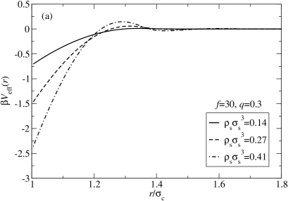
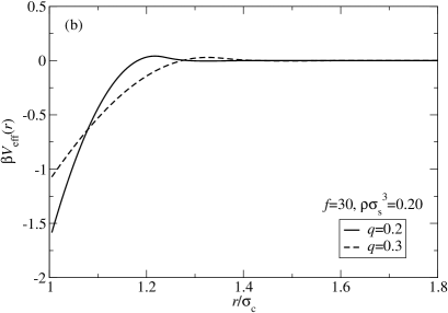
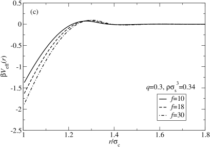
Figure 5: Effective colloid–colloid depletion potentials $V_{\rm eff}(r)$ as obtained by an inversion of the OZ relation. For details concerning the procedure, see main text. We have investigated the influence of (a) the partial star density $\rho_{\rm s}^{\rm r}=\rho_{\rm s}$, (b) the PE-star–colloid size ratio $q$, and (c) the stars’ functionality $f$ on the functional form of the interaction potential. It is evident from the plots that the presence of the stars induces an attraction between the colloids in addition to their bare hard-sphere repulsion which takes over for distances $r\leq\sigma_{\rm c}$.

Fig. 5 shows examples for the effective colloid–colloid interaction $V_{\rm eff}(r)$ for different functionalities $f$ of the stars, partial star densities $\rho_{\rm s}^{\rm r}=\rho_{\rm s}$, and PE-star–colloid size ratios $q$. As one can see from the plots, for distances $r>\sigma_{\rm c}$ the resulting depletion interaction mediated by the stars is attractive and features a slightly oscillating behaviour, while for inter-particle separations $r\leq\sigma_{\rm c}$ the bare hard-sphere repulsion remains. In particular, fig. 5(a) illustrates that the addition of PE-stars to the mixture results in both a significant increase of the depth of the attractive potential well and a further enhancement of the aforementioned oscillations but does in no way affect the range of the attraction. As can be read off from fig. 5(b), the latter is determined by the size ratio $q$ alone and grows linearly with the diameter of the stars. Furthermore, there is a measurable, indeed weak, dependence of the interaction strength on the functionality of the PE-stars: The higher the arm number $f$ gets the stronger becomes the effective attraction between two colloids, cf. fig. 5(c). All these trends are in perfect agreement with the common understanding of the physical mechanisms leading to the appearance of such an effective attraction: Due to a depletion of the PE-stars in the spatial region between a pair of colloids and dependent on the colloids’ mutual distance, they are hit asymmetrically by the stars from the inside and the outside. Consequently, the unbalanced osmotic pressure pushes the colloids together. Clearly, the absolute value of this force must grow when increasing the star density $\rho_{\rm s}$, simply because there are more collisions between PE-stars and colloids. For higher functionalities $f$, the colloid–PE-star cross interaction becomes more repulsive (see sec. 2.2), i.e., the stars push the colloids harder, thus also leading to a strengthened effective colloid–colloid attraction. And finally, the PE-stars’ diameter determines whether or not they fit into the spatial region between a pair of colloids for a given distance of the two. Hence, the size ratio $q$ controls if the stars are expelled from the said region of space, or to put it in other words, for what scope of inter-colloidal separations depletion actually takes place. Accordingly, the range of the effective force can be altered by changing $q$.

The occurrence of oscillations of the effective potential $V_{\rm eff}$ obviously means that the attractive minimum is followed by a repulsive barrier whose height is set by the concentration of PE-stars in the mixture, see above. In particular, it grows upon addition of stars to the system and such behaviour could in case of distinctly high and broad maxima in principle lead to micro-phase separation, i.e., cluster formation [47, 48, 49, 50, 51]. But for the physical system we examine and the range of parameters we investigate, the barrier remains anyway rather low and narrow. Micro-phase separation is therefore not likely to happen. Instead, the type of effective colloid–colloid attractions at hand, i.e., an attractive potential valley together with a nearly vanishing or at least less-pronounced repulsive barrier, forces the system to develop long-range fluctuations upon an increase of the PE-star concentration, consequently favoring the possibility of a fluid–fluid demixing transition of the two-component mixture. Such behaviour is frequently observed in, e.g., colloid–polymer mixtures [52, 53, 54]. Thus, when considering the phase behaviour of our system by calculating its binodals, we expect to find evidence for macro-phase separation. This supposition will be endorsed by the results of the following section, too.

4.2 Structure of the mixture

Before switching over to a presentation of the demixing binodals as obtained via the procedure described in detail in Sec. 3 of this paper, i.e., initially calculating the Gibbs free energy $g(x_{\rm s})$ with both the temperature $T$ and the pressure $P$ kept fixed and subsequently identifying the sought-for coexisting fluid phases using Maxwell’s common tangent construction for the concave parts of that function (see, in particular, figs. 3 and 4), it is useful to study partial pair correlation functions $g_{ij}(r)$ and corresponding structure factors $S_{ij}(k)$ ($i,j={\rm c,s}$) first. Since these quantities completely describe the pair structure of the system, we are able to gain detailed insight into the physics and phase behaviour of the mixture and to discover, in addition to the findings of the previous Sec. 4.1, more evidence that it is reasonable to expect an mixing–demixing transition.

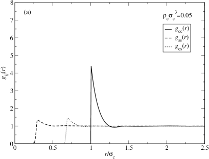
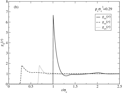
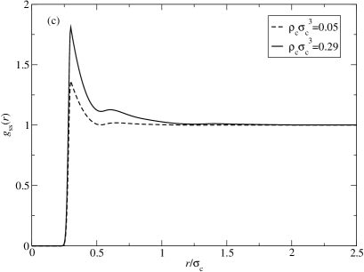
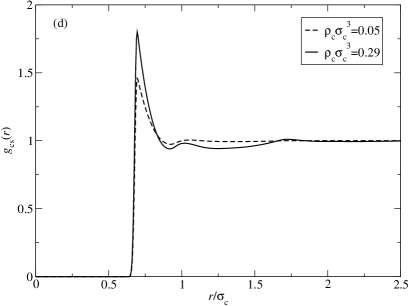
Figure 6: Partial radial distribution functions $g_{ij}(r)$ ($i={\rm c,s}$) for PE-stars with $f=30$ arms, star–colloid size ratio $q=0.3$, fixed PE-star density $\rho_{\rm s}\sigma_{\rm s}^{3}=0.27$, and colloidal densities of (a) $\rho_{\rm c}\sigma_{\rm c}^{3}=0.05$ or (b) $\rho_{\rm c}\sigma_{\rm c}^{3}=0.29$. For the same value of the stars’ partial density, the remaining two parts of the figure illustrate the detailed shape and the $\rho_{\rm c}$-dependence of (c) the star–star correlation function $g_{\rm ss}(r)$ and (d) the cross-correlation function $g_{\rm cs}(r)$. For an in-depth discussion and interpretation of the results, we refer the reader to the main text.

Fig. 6 shows the partial radial distribution functions $g_{ij}(r)$ for typical parameters, namely a colloid–PE-star mixture with a size ratio of $q=0.3$ and the PE-stars having $f=30$ arms each. We show results for different mixture compositions, i.e., varying partial densities for both species as indicated in the plots. Figs. 6(a) and (b), on the one hand, depict the decisive length scales of the problem or, equivalently, the typical ranges of the underlying pair potentials as set by the the sizes of colloids and PE-stars, respectively. The distinct height of the colloid–colloid contact value $g_{\rm cc}(\sigma_{\rm c})$ and its further rise upon increasing the PE-star density (not shown in our figures) is an obvious manifestation of the mainly attractive character of the effective colloid–colloid interactions. In this respect, we again refer the reader to Sec. 4.1 and, in particular, eq. (32) mathematically describing the inversion procedure for the OZ relation. On the other hand, when taking a closer look to the whole set of pair correlation functions, we find various signs pointing towards the supposable occurrence of a demixing transition. The main peaks of both $g_{\rm ss}(r)$ and $g_{\rm cc}(r)$ gain in height when adding colloids to the system, while the peak height of the cross-correlation function $g_{\rm cs}(r)$ remains essentially the same, see figs. 6(a), (b) and (d). In addition, figs. 6(c) and (d) show an enhancement in the star–star pair correlations and an concurrent depletion in the colloid–star correlations for raising colloid densities. The intervals of distances affected are remarkably broad, both the range of the enhancement and the depletion are of the order of the colloid size, not the much smaller star size. Altogether, these features show the tendency of colloids as well as stars to seek spatial proximity of their own species while sort of avoiding the other one and we may expect macroscopic regions rich in the one and poor in the other species to be formed provided the partial densities, in particular of the colloids, are sufficiently high.

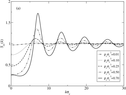
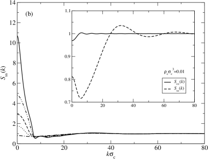
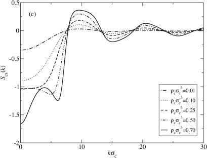
Figure 7: Examples of the partial structure factors (a) $S_{\rm cc}(k)$, (b) $S_{\rm ss}(k)$, and (c) $S_{\rm cs}(k)$ for PE-star functionality $f=18$, size ratio $q=0.2$, fixed density of the stars $\rho_{\rm s}\sigma_{\rm s}^{3}=0.12$, and several values of the colloidal density $\rho_{\rm c}\sigma_{\rm c}^{3}$, i.e., different mixture compositions. Please note that the line styles in the main plot of part (b) refer to the same parameters as explained in the legends of parts (a) and (c), respectively. The inset in (b) addresses a comparison between the colloid–colloid and the star–star structure factors for the aforementioned star density and a typical value of the colloid density (indicated in the plot) and thereby illustrates the huge difference in the structural length scales of the two species.

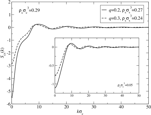
Figure 8: Comparison of the cross structure factors $S_{\rm cs}(k)$ for $f=30$ and the two different size ratios investigated, $q=0.2$ and $q=0.3$. The PE-star partial densities were chosen to be almost the same in both cases, i.e., $\rho_{\rm s}\sigma_{\rm s}^{3}=0.27$ and $\rho_{\rm s}\sigma_{\rm s}^{3}=0.24$, respectively. The corresponding colloid densities are $\rho_{\rm c}\sigma_{\rm c}^{3}=0.29$ (main plot) and $\rho_{\rm c}\sigma_{\rm c}^{3}=0.05$ (inset). Upon varying the size ratio, the peak positions shift and the $(k=0)$-values of the partial structure factors shown change significantly while there is no remarkable effect on the different peaks’ height.

Fig. 7 illustrates the typical shape of the partial structure factors $S_{ij}(k)$. Here, we chose the parameters as follows: the PE-star functionality is $f=18$, we set the size ratio to $q=0.2$, fixed the density of the stars as $\rho_{\rm s}\sigma_{\rm s}^{3}=0.12$, and considered several values of the colloidal density $\rho_{\rm c}\sigma_{\rm c}^{3}$. When comparing the three main plots of the figure, the first finding is that the locations of the different Lifshitz lines in density space strongly vary. These lines mark the respective structure factors’ cross-over between a regime where they display a local minimum in the long wavelength limit $k\rightarrow 0$ and a region where the behaviour changes to developing a local maximum for the same $k$-values. While for the given amount of stars in the system the star–star Lifshitz line is obviously immediately crossed for practically arbitrary low colloid concentrations [fig. 7(b)], we need an noticeably increased partial colloid density lying in the range of about $\rho_{\rm c}\sigma_{\rm c}^{3}\approx 0.25\ldots 0.5$ for the colloid–star structure factor to experience such cross-over [fig. 7(c)]. In case of the colloid–colloid structure factor, the corresponding values of the colloid density are even higher, about $\rho_{\rm c}\sigma_{\rm c}^{3}\approx 0.7$ for the parameters used here [fig. 7(a)]. Another indication of the demixing transition we are searching for within the scope of this paper and that is expected to occur upon adding more and more colloids and stars to the binary mixture is the tendency of all partial structure factors to diverge in the aforementioned long wavelength limit, i.e., $S_{\rm cc}(k\rightarrow 0)\rightarrow+\infty$, $S_{\rm ss}(k\rightarrow 0)\rightarrow+\infty$ and $S_{\rm cs}(k\rightarrow 0)\rightarrow-\infty$, thus demonstrating that we approach the spinodal line. The inset in fig. 7(b) was included in order to again demonstrate the huge difference in the structural length scales of the two species present in the mixture. The pre-peak in the cross structure factor $S_{\rm cs}(k)$ is without any direct physical interpretation, while pre-peaks in the intra-species structure factors would evince micro-phase separation [47, 48, 49, 50, 51]. Since the latter peaks are completely absent in our case, we may once more conclude that the system is expected to macro-phase separate instead of forming clusters.

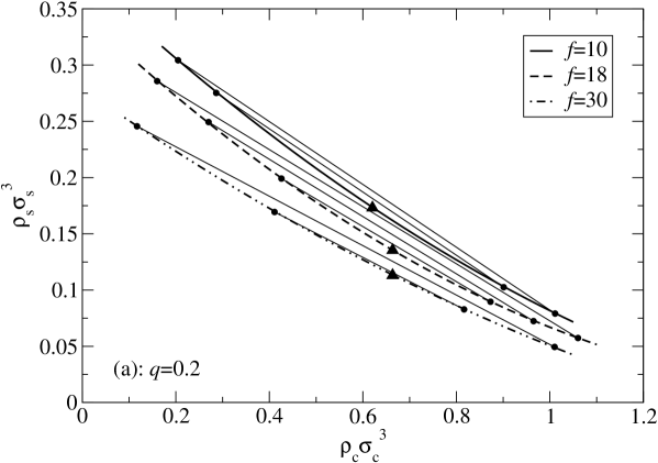
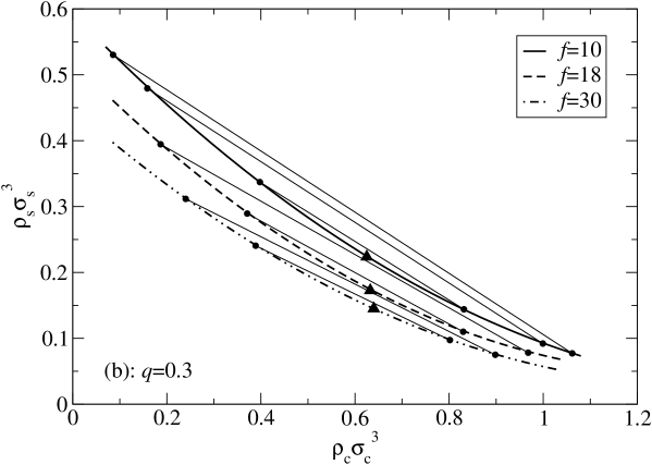
Figure 9: Demixing binodals calculated according to the procedures introduced in the main text for (a) $q=0.2$ and (b) $q=0.3$, and different values of the PE-stars’ functionality $f$. In order to illustrate the coexisting colloid-poor and colloid-rich phases, we additionally show several tie lines. In this connection, please note that we in fact used much more such point pairs in order to obtain the binodal lines and not only the shown ones. Based on the full sets of coexisting fluid phases we computed, we made rough estimates for the positions of the respective critical points in the $\rho_{\rm c}$-$\rho_{\rm c}$ plane, represented by the filled triangles.

Finally, fig. 8 depicts the $q$-dependence of the cross structure factors for $f=30$ and two different values of the colloid density $\rho_{\rm c}\sigma_{\rm c}^{3}$ (main plot and inset). For both size ratios investigated, the star densities $\rho_{\rm s}\sigma_{\rm s}^{3}$ are chosen to be almost the same. As obvious from the plots, a change in $q$ only affects the peak positions and the depth of the local minimum for $k\rightarrow 0$, but there is no significant influence on the peak heights of the functions. This is in agreement with the findings for the $q$-dependence of the effective colloid–colloid interactions, see fig. 5, and essentially means that the size ratio $q$ is crucial for determining the typical structural length scales, but hardly for how pronounced this structure is.

4.3 Fluid-fluid phase equilibria

After having found plenty of evidence in our hitherto analysis for a mixing–demixing transition taking place for certain ranges of partial densities $\rho_{i}\sigma_{i}^{3}$, we finally come to a more quantitative description based on the corresponding binodals obtained as explained above. In fig. 9 we show the obtained demixing binodals for size ratios $q=0.2$ [fig. 9(a)] and $q=0.3$ [fig. 9(b)] and for different PE-star functionalities $f$, as denoted in the legend boxes. In addition, we connected some of the point pairs used to compute the binodals and representing coexisting colloid-rich and colloid-poor phases by tie lines. Concerning the mutual positions of the binodals in the density plane, it can be seen that they shift towards higher PE-star concentrations upon increasing the size ratio $q$ and/or decreasing the PE-stars’ functionality $f$. This characteristic behaviour is in agreement with previous studies of binary mixtures of colloids and neutral polymer stars [33]. The filled triangles in fig. 9 denote rough estimates for the respective critical points’ positions determined graphically by taking the tie lines into account. The critical points move towards slightly lower colloid densities when lowering the PE-stars’ arm number, whereas there is no significant effect of altering the size ratio.

The star densities $\rho_{\rm s}\sigma_{\rm s}^{3}$ that bring about a demixing instability are typically higher for the case $q=0.3$ than for the case $q=0.2$. This looks counterintuitive at first sight, since one expects that larger PE-stars will destabilise the mixture earlier. In order to put the numbers in their appropriate context, it is useful to employ the picture of the effective colloid-colloid potential, which includes a star-induced attraction. Here, the range and depth of this attraction steer the occurrence of the demixing binodal, which is equivalent to a separation between a colloidal fluid and a colloidal gas. The natural length scale in this picture is the colloid diameter $\sigma_{\rm c}$; concomitantly, the physically relevant density in making comparisons between the $q=0.2$ and the $q=0.3$ cases should be scaled with the colloid size: $\rho_{\rm s}\sigma_{\rm c}^{3}=q^{-3}\rho_{\rm s}\sigma_{\rm s}^{3}$. It can be easily seen that the additional prefactor $q^{-3}$ renders the rescaled star densities for $q=0.3$ indeed lower than the ones for $q=0.2$, in agreement with the intuitive expectations.

The volume terms for the integrated out counterions [55, 56, 57] do not affect the phase boundaries, since, under the assumption of full absorbing in the stars’ interiors, they are simply proportional to the number $N_{\rm s}$ of the latter [11] and thus they cause a trivial shift of the stars’ chemical potential, without affecting the solution’s osmotic pressure [58]. Finally, we mention that we did not consider the competition between the demixing binodals and the crystallization of the colloids. The investigation of the system’s solid states lies beyond the scope of this work. The trends found for the $f$- and $q$-dependences are comparable to the colloid–star polymer case mentioned above. Although the underlying pair potentials are different to a certain degree, a closer inspection to the full phase diagrams in Ref. [33] can give hints regarding the stability of the binodals against preemption by the freezing lines. Provided the positions of the freezing lines are not too different here, it seems to be reasonable to assume based on such a comparison that our demixing lines will survive at least for the larger size ratio between stars and colloids. Nevertheless, the existence of a demixing binodal, even in the case that the latter is preempted by crystallization, has important consequences for the time scales involved in the dynamics of crystallization [59, 60].

5 Summary and conclusions

We have put forward a coarse-grained description of mixtures between neutral, spherical, hard colloids and multiarm polyelectrolyte stars of size smaller than the colloidal particles. Effective interactions between the constituent particles have been employed throughout, allowing for a mesoscopic description that leads to valuable information on the structure and thermodynamics of the two-component mixture. The cross interaction, which has been derived in this work, is sufficiently repulsive to bring about regions of instability in the phase diagram and leading thereby to macroscopic, demixing phase behaviour. This, in turn, can be rationalised by means of the depletion potentials between the colloids, which are induced by the stars, and feature attractive tails akin to those encountered in usual colloid-polymer mixtures.

The form of the cross interaction plays a crucial role in determining stability and can, by suitable tuning, completely change the behaviour of the mixture from macroscopic phase separation to microphase structuring with a finite wavelength. In this respect, a very promising direction of investigation is to allow for the colloids to carry a charge opposite to that of the arms of the polyelectrolyte stars. Preliminary results already indicate a rich variety of resulting complexation morphologies between the two constituents [61]. A detailed investigation of the complexation characteristics and the morphologies of the ensuing macroscopic phases is the subject of ongoing work.

References

References

- [1] Pincus P 1991 Macromolecules 24 2912
- [2] Wang H and Denton A R 2004 Phys. Rev. E 70 041404
- [3] Borisov O V and Zhulina E B 1997 J. Phys. II (Paris) 7 499
- [4] Borisov O V and Zhulina E B 1998 Eur. Phys. J. B 4 205
- [5] Klein Wolterink J, Leermakers F A M, Fleer G J, Koopal L K, Zhulina E B and Borisov O V 1999 Macromolecules 32 2365
- [6] Klein Wolterink J, van Male J, Cohen Stuart M A, Koopal L K, Zhulina E B and Borisov O V 2002 Macromolecules 35 9176
- [7] Jusufi A, Likos C N and Löwen H 2002 Phys. Rev. Lett. 88 018301
- [8] Jusufi A, Likos C N and Löwen H 2002 J. Chem. Phys. 116 11011
- [9] Denton A R 2003 Phys. Rev. E 67 011804
- [10] Likos C N, Hoffmann N, Jusufi A and Löwen H 2003, J. Phys.: Condens. Matter 15 S233
- [11] Hoffmann N, Likos C N and Löwen H 2004 J. Chem. Phys. 121 7009
- [12] Furukawa T and Ishizu K 2005 Macromolecules 38 2911
- [13] Gorodyska G, Kiriy A, Minko S, Tsitsilianis C and Stamm M 2003 Nano Letters 3 365
- [14] Serpe M J, Kim J and Lyon L A 2004 Adv. Mater. 16 184
- [15] Kim J, Serpe M J and Lyon L A 2005 Angew. Chem. Int. Ed. 44 1333
- [16] Konieczny M and Likos C N 2006 J. Chem. Phys. 124 214904
- [17] Fortini A, Dijkstra M and Tuinier R 2005 J. Phys.: Condens. Matter 17 7783
- [18] Jusufi A, Likos C N and Ballauff M 2004 Colloid Polym. Sci. 282 910
- [19] Manning G S 1969 J. Chem. Phys. 51 924
- [20] Konieczny M, Likos C N and Löwen H 2004 J. Chem. Phys. 121 4913
- [21] Konieczny M and Likos C N 2006 Macromolecular Symposia in press
- [22] Jusufi A, Dzubiella J, Likos C N, von Ferber C and Löwen H 2001 J. Phys.: Condens. Matter 13 6177
- [23] Hansen J-P and McDonald I R Theory of Simple Liquids, 2nd ed. (London: Academic Press 1986)
- [24] Hansen J-P and Löwen H 2000 Annu. Rev. Phys. Chem. 51 209
- [25] Lebowitz J L and Rowlinson J S 1964 J. Chem. Phys. 41 133
- [26] Rogers F J and Young D A 1984 Phys. Rev. A 30 999
- [27] Biben T and Hansen J P 1991 J. Phys.: Condens. Matter 3 65
- [28] Kirkwood J G and Buff F P 1951 J. Chem. Phys. 19 774
- [29] Ashcroft N W and Stroud D 1978 Solid State Phys. 33 2 (Academic: New York)
- [30] Likos C N and Ashcroft N W 1992 J. Chem. Phys. 97 9303
- [31] Biben T and Hansen J-P 1991 Phys. Rev. Lett. 66 2215
- [32] Bathia A B and Thornton D E 1970 Phys. Rev. B 2 3004
- [33] Dzubiella J, Likos C N and Löwen H 2002 J. Chem. Phys. 116 9518
- [34] Rowlinson J S and Swinton F L Liquids and Liquid Mixtures (London: Butterworth 1982)
- [35] Landau L D and Lifshitz E M Course of Theoretical Physics: Statistical Physics, 3rd ed. (Oxford: Pergamon Press 1980)
- [36] Carnahan N F and Starling K E 1969 J. Chem. Phys. 51 635
- [37] Archer A J, Likos C N and Evans R 2002 J. Phys.: Condens. Matter 14 12031
- [38] Mayer C, Likos C N and Löwen H 2004 Phys. Rev. E 67 0414025
- [39] Dzubiella J, Likos C N and Löwen H 2002 Europhys. Lett. 58 133
- [40] Méndez-Alcaraz J M and Klein R 2000 Phys. Rev. E 61 4095
- [41] König A and Ashcroft N W 2001 Phys. Rev. E 63 041203
- [42] D’Amico I and Löwen H 1997 Physica A 237 25
- [43] Allahyarov E, D’Amico I and Löwen H 1998 Phys. Rev. Lett. 81 81 1334
- [44] Allahyarov E and Löwen H 2001 J. Phys.: Condens. Matter 13 L277
- [45] Attard P 1989 J. Chem. Phys. 91 3083
- [46] Moreno A J and Colmenero J 2006 Phys. Rev. E 74 021409
- [47] Mossa S, Sciortino F, Tartaglia P and Zaccarelli E 2004 Langmuir 20 10756
- [48] Sciortino F, Mossa S, Zaccarelli E and Tartaglia P 2004 Phys. Rev. Lett. 93 055701
- [49] Sear R P and Gelbart W M 1999 J. Chem. Phys 110 4582
- [50] Imperio A and Reatto L 2006 J. Chem. Phys. 124 164712
- [51] Imperio A and Reatto L 2004 J. Phys.: Condens. Matter 16 3769
- [52] Vink R L C, Jusufi A, Dzubiella J, and Likos C N 2005 Phys. Rev. E 72 030401(R)
- [53] Lo Verso F, Pini D and Reatto L 2005 J. Phys.: Condens. Matter 17 771
- [54] Lo Verso F, Vink R L C, Pini D and Reatto L 2006 Phys. Rev. E 73 061407
- [55] van Roji R and Hansen J-P 1997 Phys. Rev. Lett. 79 3082
- [56] van Roji R, Dijkstra M and Hansen J-P 1999 Phys. Rev. E 59 2010
- [57] Denton A R 2000 Phys. Rev. E 62 3855
- [58] Likos C N 2001 Phys. Rep. 348 267
- [59] ten Wolde P R and Frenkel D 1997 Science 277 1975
- [60] Frenkel D 1999 Physica A 263 26
- [61] Konieczny M, Jusufi A and Likos C N unpublished