Longest increasing subsequence as expectation of a simple nonlinear stochastic PDE with a low noise intensity

Abstract

We report some new observation concerning the statistics of Longest Increasing Subsequences (LIS). We show that the expectation of LIS, its variance, and apparently the full distribution function appears in statistical analysis of some simple nonlinear stochastic partial differential equation (SPDE) in the limit of very low noise intensity.

I Introduction

Last decade is marked by a breakthrough in the solution of a classical probabilistic problem, known as ”Ulam problem” discussed in the mathematical literature over the years Ulam . The general setting of the Ulam problem is as follows. Take the unit interval $[0,1]$ and pick up from it one after another $N$ random numbers ($N\gg 1$) with uniform probability distribution. Having the sequence of $N$ random numbers, one can extract from it the longest increasing subsequence (LIS) of $k$ elements. The entries of this subsequence are not obliged to be the nearest neighbors. There are two basic questions of interest: i) what is the expectation $\left<k(N)\right>$ of LIS; and ii) what are the fluctuations of the mean length of LIS. The first question has been answered in 1975 by Vershik and Kerov VK who have shown that $\left<k(N)\right>=2\sqrt{N}$ for $N\gg 1$. They derived this result by mapping the expectation of the LIS to the expectation of the first row of ensemble of Young tableaux over the Plancherel measure. If the initial random sequence contains repeated numbers, then the first line of the Young tableau corresponds to the longest nondecreasing subsequence.

The progress in treatment of fluctuations of LIS was the subject of recent investigations tracy ; deift ; johannson ; okunkov ; aldous ; spohn . In these works an exact asymptotic form of a properly normalized full limiting distribution has been established (the so-called Tracy–Widom distribution) of the first row of the Young tableau over the Plancherel measure by mapping to the distribution of the largest eigenvalues of some classes of random matrices tracy . In particular it has been shown that the properly normalized variance of LIS has for $N\gg 1$ the asymptotic scaling form ${\rm Var}[k(N)]\equiv\left<k^{2}(N)\right>-\left<k(N)\right>^{2}=cN^{1/3}$, where $c=\left<[\chi-\left<\chi\right>]^{2}\right>=0.8132...$ and $\chi$ has the Tracy–Widom distribution for the Gaussian Unitary Ensemble.

We would like also to point out a deep connection between the distributions of edge states of random matrices and of statistical characteristics of some random growth models. In one of the most stimulating work johannson , it has been shown that a (1+1)–dimensional model of directed polymers in random environment, which is in the KPZ universality class, has the Tracy–Widom distribution for the scaled height (energy). Around the same time the authors of spohn have found an exact mapping between a specific polynuclear growth (PNG) model and the LIS problem. The same Tracy–Widom distribution was reported in another class of (1+1)–dimensional growth models called ”oriented digital boiling” model GTW .

In our work we report some new observation concerning the statistics of longest increasing subsequences. Namely, we show that the expectation of LIS, its variance, and apparently the full distribution function appears in a statistical analysis of some properly scaled simple nonlinear stochastic partial differential equation (SPDE) in a limit of very low noise intensity.

The paper is organized as follows. In Section II we introduce all the necessary definitions. In particular, we describe LIS as the hight profile of some uniform discrete growth problem with nonlocal long–ranged interactions. In Section III we consider the discrete short–ranged asymmetric uniform growth process and derive the corresponding continuous space–time SPDE for the height profile. In Section IV we show that the properly scaled limit of an infinitely small noise in the derived SPDE adequately describes the growth with long–ranged interactions, i.e. the statistics of LIS. The discussion and conclusions are collected in Section V.

II LIS as a height profile in a uniform asymmetric non-local growth process

The standard construction of a Young tableau for the set of real numbers is realized via the well known Robinson–Schensted–Knuth algorithm (RSK) which can be found in many textbook on representation theory, and for example, in rsk . The RSK algorithm ensures that the first row of the corresponding Young tableau would be the Longest Increasing Subsequence (LIS) for a given set of numbers. To be specific, consider the example of $N=8$ numbers: $4,4,3,6,7,3,4,2$ taken at random with uniform probability distribution from the support $\{1,...,9\}$. Following the RSK algorithm of the Young tableau construction, we get the Young tableau shown in Fig.1a. Let us describe now more geometrically obvious construction of LIS which refers to the discrete uniform asymmetric ballistic deposition of elementary cells with long–ranged interactions. This construction has appeared for the first time in maj_nech1 .

Consider the (1+1)D model of ballistic deposition in which the columnar growth occurs sequentially on a linear substrate consisting of $L$ columns with free boundary conditions. The time $t$ is discrete and increases by $1$ with every deposition event. We start with the flat initial condition, i.e., an empty substrate at $t=0$. At any stage of the growth, a column (say the column $m$) is chosen at random with probability $p=\frac{1}{L}$ and a ”cell” is deposited there which increases the height of this column by one unit: $h_{m}\to h_{m}+1$. Once this ”cell” is deposited, it screens all the sites at the same level in all the columns to its right from future deposition, i.e. the heights at all the columns to the right of the column $m$ must be strictly greater than or equal to $h_{m}+1$ at all subsequent times. Formally such a growth is implemented by the following update rule. If the site $m$ is chosen at time $t$ for deposition, then

$$h_{m}(t+1)={\rm max}\{h_{m}(t),h_{m-1}(t),\dots,h_{1}(t)\}+1$$ (1)

The model is anisotropic and long–ranged and evidently even the average height profile $\left<h_{m}(t)\right>$ depends nontrivially on both the column number $k$ and time $t$. Let us demonstrate now the a bijection between the longest nondecreasing subsequence in the sequence of $N$ random numbers uniformly taken from the support $\{1,2,3,...L\}$ and the height in the uniformly growing heap with anisotropic infinite–ranged interactions in a bounding box containing $L$ columns.

This bijection is defined by assigning the first line in the Young tableau to the ”most top” (or ”visible” from the left–hand side) blocks—see the Fig.1b. For the configuration shown in Fig.1 we have the sequence of $N=8$ numbers: $4,4,3,6,7,3,4,2$ taken at random from the set $\{1,...,9\}$ (there are $L=9$ columns in the box). The ”visible” blocks define the longest nondecreasing subsequence (LNS): $2,3,4,7$. To be exact, if there are few LNSs, our construction extracts one of them – exactly as in the RSK scheme.

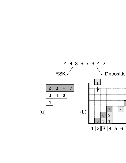
Figure 1: (a) Young tableau; (b) Asymmetric Ballistic Deposition.

As one can see in Fig.1, the first line in the Young tableau (1) exactly matches the ”most top” subsequence defined in our model and the distribution of the maximal height of a heap coincides with the distribution of the longest nondecreasing subsequence.

III Short–ranged asymmetric ballistic growth and its continuous limit

Consider a one–dimensional discrete model of ballistic deposition with asymmetric (one–sided) next–nearest–neighboring (NNN) interactions

$$h_{j}(t+1)=\max\{h_{j}(t),h_{j-1}(t)\}+\eta_{j}(t)$$ (2a)

where $$h_{j}(t) j t \eta_{j}(t)$$ is the height of a surface at the lattice position and time (the time is discrete as well) and is a telegraph–like uncorrelated noise:

$$\eta_{j}(t)=\left\{\begin{array}[]{ll}1&\mbox{with probability $p$}\vskip 6.0pt plus 2.0pt minus 2.0pt\\ 0&\mbox{with probability $1-p$}\end{array}\right.$$ (2b)

where

$$\begin{cases}\overline{\eta_{j}(t)}=p\vskip 6.0pt plus 2.0pt minus 2.0pt\\ \overline{\Big{(}\eta_{j}(t_{1})-\overline{\eta_{j}(t_{1})}\Big{)}\,\Big{(}\eta_{m}(t_{2})-\overline{\eta_{m}(t_{2})}\Big{)}}=p(1-p)\,\delta_{j,m}\,\delta_{t_{1},t_{2}}\end{cases}$$ (2c)

The bar denotes averaging over the distribution (2b). Equations (2a)–(2c) completely describe the updating rules for the NNN discrete ballistic deposition with the asymmetric interactions shown in Fig.2.

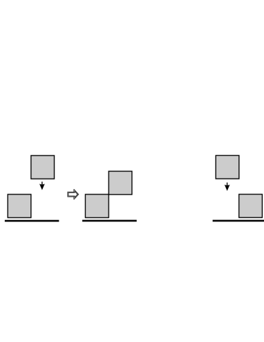
Figure 2: Updating rules for the asymmetric NNN ballistic deposition defined in Eq.(2a).

In order to derive a continuous model corresponding to (2a), We represent the $\max\{...\}$ operator in (2a) at time $t$ by a sign–function ${\rm sign}[z]$:

$$\begin{array}[]{rl}\max\{h_{j-1},h_{j}\}=&\frac{1}{2}h_{j-1}\left(1+\mbox{sign}\left[h_{j-1}-h_{j}\right]\right)\vskip 6.0pt plus 2.0pt minus 2.0pt\\ +&\frac{1}{2}h_{j}\left(1+\mbox{sign}\left[h_{j}-h_{j-1}\right]\right)\end{array}$$ (3)

where

$$\mbox{sign}[z]=\begin{cases}+1&\mbox{for $z>0$}\\ -1&\mbox{for $z<0$}\end{cases}$$

Substituting (3) into (2a) we get after some simple algebra

$$\begin{array}[]{l}h_{j}(t+1)-h_{j}(t)=-\frac{1}{2}(h_{j}(t)-h_{j-1}(t))\vskip 6.0pt plus 2.0pt minus 2.0pt\\ \hskip 14.22636pt+\frac{1}{2}(h_{j}(t)-h_{j-1}(t))\mbox{sign}[h_{j}(t)-h_{j-1}(t)]+\eta_{j}(t)\end{array}$$ (4)

In the last expression one can easily identify the finite–difference derivatives. Denoting the spatial and temporal increments by $\Delta x$ and $\Delta t$ and taking into account that $\mbox{sign}[az]=\mbox{sign}[z]$ (for $a>0$), we arrive at the following expression

$$\begin{array}[]{rl}\partial_{t}h(x,t)=&-\frac{1}{2}\frac{\Delta x}{\Delta t}\partial_{x}h(x,t)\left(1-\mbox{sign}\left[\partial_{x}h(x,t)\right]\right)\vskip 6.0pt plus 2.0pt minus 2.0pt\\ &+\frac{1}{\Delta t}\eta(x,t)\end{array}$$ (5)

where $\partial_{t}h(x,t)$ and $\partial_{x}h(x,t)$ denote the partial derivatives of $h(x,t)$ with respect to $t$ and $x$ correspondingly. Setting in (5) $\Delta t=\Delta x=1$ we arrive at the nonlinear stochastic partial differential equation (SPDE) which is a continuous analog of the discrete Asymmetric Ballistic Deposition described by (2a). The noise in (5) is still defied by (2b)–(2c).

It is known katzav that symmetric Ballistic Deposition model with NNN interactions in the continuous limit has some relevance to KPZ equation kpz . For better comparison of the KPZ equation with our SPDE one, rewrite (5) as follows:

$$\partial_{t}h(x,t)=\frac{1}{2}\left|\partial_{x}h(x,t)\right|-\frac{1}{2}\partial_{x}h(x,t)+\eta(x,t)$$ (6a)

or, equivalently,

$$\partial_{t}h(x,t)=\left\{\begin{array}[]{ll}\displaystyle\eta(x,t)-\partial_{x}h(x,t)&\mbox{if $\quad\displaystyle\partial_{x}h(x,t)<0$}\vskip 6.0pt plus 2.0pt minus 2.0pt\\ \displaystyle\eta(x,t)&\mbox{if $\quad\displaystyle\partial_{x}h(x,t)>0$}\end{array}\right.$$ (6b)

with $\eta(x,t)$ given by (2b)–(2c). One sees that the stochastic equation (6a) does not contain a diffusion term and is very different from the KPZ one. However, as will be shown below, the expectation $\left<h(x,t)\right>$ of Eq.(6a) converges for $t\gg 1$ and $x\gg 1$ to the expectation of LIS for a noise $\eta(x,t)$ with very small intensity $p$ ($p<L^{-2}$). The same is valid for the variance, $\mbox{Var}[h(x,t)]$, which demonstrates the KPZ scaling behavior. All that allows us to conjecture that the full distribution of $h(x,t)$ for small $p$ converges to a Tracy–Widom distribution of LIS. Let us note that the structure of Eq.(6b) ”ideologically” resembles the structure of the one–dimensional Barenblatt model for the field $u(x,t)$ with different diffusion constants for $\partial_{t}u(x,t)>0$ and $\partial_{t}u(x,t)<0$ barenblatt .

IV SPDE in the infinitely rare noise regime and LIS

In this Section we show that the limit of a telegraph–like noise with small intensity in the stochastic partial differential equation (6a) for the ”height” function $h(x,t)$ has LIS statistics. To do that, it is convenient to describe LIS in terms of (1+1)D Ballistic Deposition (BD) set by Eq.(1).

Let us begin with the limiting case of absence of any noise in (6a). The noiseless equation (6a) is invariant under the scaling transformation $h(x,t)\to h(ax,at)$ for any $a$. Rewriting (6a) in a finite–difference form on the lattice, we have:

$$\begin{array}[]{rl}h(x,t+\Delta t)=h(x,t)&+\frac{1}{2}\Delta t\left|\frac{h(x,t)-h(x-\Delta x,t)}{\Delta x}\right|\vskip 6.0pt plus 2.0pt minus 2.0pt\\ &-\frac{1}{2}\Delta t\left(\frac{h(x,t)-h(x-\Delta x,t)}{\Delta x}\right)\end{array}$$ (7)

We can set $\Delta t=\Delta x=1$ and $x=j$ on the interval $0\leq j\leq L$ without any loss of generality. The noiseless system defined by Eq.(7) has a characteristic time scale $\tau\sim L$ of reaching the equilibrium. Hence, after $t$ time steps, where $t>\tau$, the system described by Eq.(7) reaches its stationary state generating a nondecreasing staircase–like profile from any initial state. This can be seen recursively:

$$\left\{\begin{array}[]{ll}h(j,t+1)=h(j-1,t)&\mbox{if $h(j-1,t)>h(j,t)$}\vskip 6.0pt plus 2.0pt minus 2.0pt\\ h(j,t+1)=h(j,t)&\mbox{if $h(j-1,t)<h(j,t)$}\end{array}\right.$$ (8)

Since (8) is valid for any $0\leq j\leq L$, after $t\sim L$ time steps, if in the initial state $h(j=L,t=0)<h(j=1,t=0)$ then the heights at $x=L$ and $x=1$ equalize: $h(j=L,t)=h(j=1,t)$. This signals the appearance of effective long–ranged spatial correlations in the system on characteristic time scales of $\tau\sim L$.

To show the equivalence of SPDE and LIS in a noisy regime with small intensity, it is convenient to introduce the enveloping functions $r_{m}(t)$ and $r(x,t)$ for long–ranged (LR) BD and SPDE correspondingly:

$$\left\{\begin{array}[]{rcll}r_{m}(t)&=&\max\{h_{m}(t),\dots,h_{1}(t)\}&\mbox{LR BD (Eq.(\ref{eq:1})})\vskip 6.0pt plus 2.0pt minus 2.0pt\\ r(x,t)&=&\displaystyle\max_{0\leq y\leq x}\{h(y,t)\}&\mbox{SPDE}\end{array}\right.$$ (9)

If the intensity, $p$, of the noise $\eta(x,t)$ is small, after each noise event the function $h(x,t)$ has time to reach its relaxed form $r(x,t)$ before the subsequent noise contribution is added. The corresponding intensity, $p$, can be easily estimated. Namely, the mean time interval, $\tau$, between positive noise events ($\eta(x,t)=1$) for a system of size $L$ and noise intensity $p$ is $\tau\sim\frac{1}{Lp}$. In more details this question is discussed in the Appendix. Since the function $h(x,t)$ reaches the relaxed state $r(x,t)$ at $\tau>L$, we can estimate $p$ as $p<L^{-2}$. Now Eqs.(1) and (6a) can be rewritten in the unified form:

$$\left\{\begin{array}[]{rcll}h_{m}(t+1)&=&r_{m}(t)+1&\mbox{long--ranged BD Eq.(\ref{eq:1})}\vskip 6.0pt plus 2.0pt minus 2.0pt\\ h(x,t+\Delta t)&=&r(x,t)+\eta(x,t)&\mbox{SPDE with $p<L^{-2}$}\end{array}\right.$$ (10)

In this form the equivalence between long–ranged BD and SPDE in a low–intensity noise regime is clearly seen.

Thus, relying on the equivalence between statistics of LIS and low–intensity solutions of SPDE (6a), and knowing explicitly all the moments of the distribution of LIS (see, for example, johannson ), we get the following asymptotic expressions for the expectation, $\left<h(x,t)\right>$, and for the variance, ${\rm Var}[h(x,t)]\equiv\left<h(x,t)^{2}\right>-\left<h(x,t)\right>^{2}$:

$$\left<h(x,t)\right>=tp+2\sqrt{xtp}\vskip 6.0pt plus 2.0pt minus 2.0pt$$ (11)

$${\rm Var}[h(x,t)]=c(xtp)^{1/3}$$ (12)

where $h(x,t)$ is the asymptotic solution of the equation (6a) with the noise distribution (2c). In (12) $c=\left<[\chi-\left<\chi\right>]^{2}\right>=0.8132...$ and $\chi$ has the Tracy–Widom distribution for Gaussian Unitary Ensemble. Note that for $p=\frac{1}{L}$ and $x=t=L$ ($L\gg 1$) we arrive in (11) at the Vershik–Kerov result for the expectation of LIS, $\left<h(L)\right>=2\sqrt{L}$. To be rigorous, this expression is beyond our approximation since we are limited by the noise intensity $p_{\rm cr}=\frac{1}{L^{2}}$. So, it is more convenient to work with the general expressions (11)–(12).

We confirm our analytic predictions (11)–(12) by numerical computations, simulating directly the ballistic deposition process (1) and the stochastic partial differential equation (6a) with noise intensity $p=\frac{0.1}{L}$ and initial condition $h(x,t=0)=0$. Note that the intensity of the noise in our numerical simulations is $\frac{L}{10}$ times larger than the upper estimate $p\sim\frac{1}{L^{2}}$, however the agreement with theoretical results (11)–(12) is still very good. In particular, we plot in Fig.3a the average profiles $\left<h(x,t)\right>$ for long–ranged BD and SPDE as a function of $x$ ($0\leq x\leq L$) for $L=10^{3}$ at time points $t=2\times 10^{4},6\times 10^{4},10^{5}$. In the same figure we plot the analytic expression (11). In Fig.3b we plot the variance ${\rm Var}(h(x,n))=\left<h(x,t)^{2}\right>-\left<h(x,t)\right>^{2}$ as a function of $x$ for the same time points $t$. It should be noted that due to the numerical procedure of the definition of the height, the numerical computation of the variance leads to the following interpolating expression for ${\rm Var}[h(x,t)]=a(t)+c(xpt)^{1/3}$. However for $x\gg 1$ and $t={\rm const}$ we arrive asymptotically at the expression (12). That is why we compare the expression (12) with the numerical data for large $x$ only where the term $a(t)$ is negligible. Moreover, the agreement between long–ranged BD and SPDE is very good for the expectation and the variance — see Fig.2a,b.

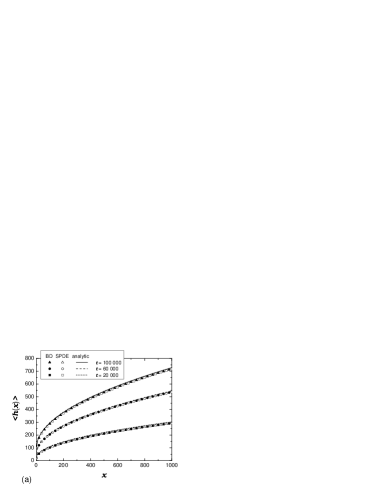
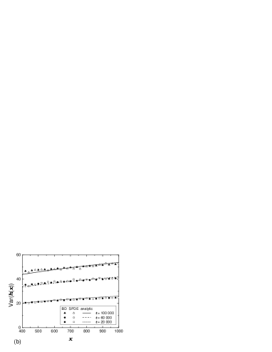
Figure 3: (a) The mean profile $\left<h(x,t)\right>$ as a function of $x$ for time points $t=2\times 10^{4},6\times 10^{4},10^{5}$ for BD and SPDE in comparison with the analytical results (11); (b) The variance ${\rm Var}(h(x,t))$ as a function of $x$ at time points $t=2\times 10^{4},6\times 10^{4},10^{5}$ for BD and SPDE in comparison with the analytic result (12). The length of the system here is $L=1000$.

V Conclusion

We have shown by the sequence of mappings that the expectation and the variance of the random profile $h(x,t)$, described by the stochastic nonlinear partial differential equation (6a) in the limit of a noise with very low intensity, coincides with the expectation (11) and the variance (12) of the longest nondecreasing subsequence of the sequence of random integers. This statement is also confirmed numerically. On the basis of the obtained results we conjecture that not only the first moments, but the full probability distribution function of the random variable $h(x,t)$ coincides with the Tracy–Widom distribution appearing in largest eigenvalue statistics of ensembles of random matrices.

Let us note that our analysis of Eq.(6a) is a bit indirect. It would be very desirable to get expectation and variance (11)–(12) of the random variable $h(x,t)$ directly from the solution of the Fokker–Planck equation which corresponds to the Langevin equation (6a). However on this way we have met some difficulties. Namely, rewrite Eq.(6a) as follows

$$\partial_{t}h(x,t)=\frac{1}{2}\left|\partial_{x}h(x,t)\right|-\frac{1}{2}\partial_{x}h(x,t)+\xi(x,t)+p$$ (13)

where $\xi(x,t)=\eta(x,t)-p$; $\overline{\xi(x,t)}=0$; $\overline{\xi(x,t)\xi(x^{\prime},t^{\prime})}=2D\delta_{x,x^{\prime}}\delta_{t,t^{\prime}}$ and $D=\frac{1}{2}p(1-p)$. Now we can write the formal expression for the Fokker–Planck variational equation for the function $W(h,t)$ (see, for example, hh ):

$$\begin{array}[]{rl}\frac{\partial W(h,t)}{\partial t}=&-\int dx\frac{\delta}{\delta h}\left\{\left(\frac{1}{2}\left|\partial_{x}h\right|-\frac{1}{2}\partial_{x}h+p\right)W(h,t)\right\}\vskip 6.0pt plus 2.0pt minus 2.0pt\\ &+D\int dx\frac{\delta^{2}}{\delta h^{2}}W(h,t)\end{array}$$ (14)

which in turn can be rearranged in a form of two coupled equations:

$$\begin{array}[]{ll}\frac{\partial W(h,t)}{\partial t}&=\int dx\left(-p\frac{\delta W(h,t)}{\delta h}+D\frac{\delta^{2}W(h,t)}{\delta h^{2}}\right)\vskip 6.0pt plus 2.0pt minus 2.0pt\\ &-\left\{\begin{array}[]{ll}\int dx\,\partial_{x}h\;\frac{\delta W(h,t)}{\delta h}&\mbox{if $\partial_{x}h<0$}\vskip 6.0pt plus 2.0pt minus 2.0pt\\ 0&\mbox{if $\partial_{x}h>0$}\end{array}\right.\end{array}$$ (15)

where we have taken into account that $\frac{\delta}{\delta h}[\partial_{x}h(x,t)]=0$.

The Fokker–Planck equation (15) corresponds to the stochastic process (6b) which can be visualized alternatively as a (2+1)–dimensional correlated growth. Using the finite–difference form (7) of (6b) on the lattice, where we set $\Delta x=\Delta t=1$ and $x=j$, we arrive at the following stochastic recursion relation

$$\begin{array}[]{l}h(x,t+1)=h(x,t)+\eta(x,t)\vskip 6.0pt plus 2.0pt minus 2.0pt\\ \hskip 28.45274pt-\left\{\begin{array}[]{ll}h(x,t)-h(x-1,t)&\mbox{if $h(x,t)<h(x-1,t)$}\vskip 6.0pt plus 2.0pt minus 2.0pt\\ 0&\mbox{if $h(x,t)>h(x-1,t)$}\end{array}\right.\end{array}$$ (16)

with the initial and boundary conditions $h(x,t=0)=h(x=0,t)=0$. Create now the initial configuration distributing the random variable $\eta(x,t)$ in the plane $x\geq 1,t\geq 1$. Since $\eta(x,t)$ takes the values 0 or 1, we can show $\eta=1$ by black unit segments as it is shown in Fig.4. The initial configuration at $t=1$ is depicted in Fig.4a. Now applying the equation (16) we can constrict recursively the configuration of the field $h(x,t)$ at subsequent time moments. Few configurations of the field $h(x,t)$ for given initial distribution of $\eta(x,t)$ is shown in Fig.4b-d for time moments $t=2,3,4$ and $x=1,...5$.

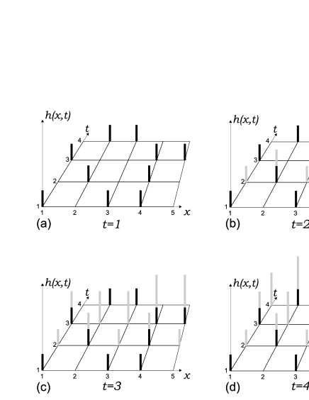
Figure 4: Visualization of the stochastic growth determined by the recursion relation (16) for $x=1,...,5$ and for several time slices $t=1$ (a), $t=2$ (b), $t=3$ (c), $t=4$ (d).

The (2+1)–dimensional stochastic growth shown in Fig.4 bijectively corresponds to the short–ranged ballistic growth considered in Section III and, hence, in the limit of small intensity $p$ should correspond to the statistics of LIS. It would be very desirable to simulate numerically directly the growth model shown in Fig.4 to check the validity of the conjectured bijection.

Appendix A Equilibration time for SPDE

In the limit of small $p$ ($p\ll 1$) the actual mean profile $\left<h(x,t)\right>$ tends to the curve $y(x,t)=tp+2\sqrt{xtp}$. However for larger values of $p$ ($p\sim 1$) the resulting profile does not have enough time to relax and hence is displaced below the curve $y(x,t)$. The question which we address here concerns the estimation of the time interval, $\tau$, between the subsequent deposition events sufficient to approach the stable solution $y(x,t)$.

We can estimate the equilibration time, $\tau$, from the following arguments. The slope of the mean profile in the stationary state is

$$\frac{\partial y(x,t)}{\partial x}=\sqrt{\frac{pt}{x}}$$ (17)

Hence, the average length of the horizonal ”plateau” is about

$$l(x)\simeq\frac{1}{\frac{\partial y(x,t)}{\partial x}}\simeq\sqrt{\frac{x}{pt}}$$ (18)

We define the equilibration time, $\tau$, as a time $t$ in (18) during which the length $l(x)$, of the plateau becomes that of the order of the system size, $L$. Substituting for $x$ in (18) the maximal value $x=L$, we arrive at the following estimate

$$L\simeq\sqrt{\frac{L}{p\tau}}$$

what gives us

$$\tau\simeq\frac{1}{Lp}$$ (19)

Comparing the equilibration time (19) with the characteristic time of the system relaxation, $\tau\sim L$, we arrive at the estimate for the critical noise intensity, $p_{\rm cr}$,

$$p_{\rm cr}\simeq\frac{1}{L^{2}}$$

below which the stochastic partial differential equation (6a) has long–ranged behavior typical for the LIS problem.

References

- (1) S.M. Ulam, Modern Mathematics for the Engineers, ed. by E.F. Beckenbach (McGraw-Hill: New York, 1961), p. 261
- (2) A.M. Vershik and S.V. Kerov, Sov. Math. Dokl. 18, 527 (1977)
- (3) C.A. Tracy and H. Widom, Comm. Math. Phys. 159, 151 (1994); 177, 727 (1996); For a review see Proceedings of the International Congress of Mathematicians, Beijing 2002, Vol. I, ed. Li Tatsien, Higher Education Press, Beijing 2002, p. 587
- (4) J. Baik, P. Deift, and K. Johansson, J. Amer. Math. Soc. 12, 1119 (1999)
- (5) K. Johansson, Comm. Math. Phys. 209, 437 (2000)
- (6) A. Okounkov, N. Reshetikhin, J. of Am. Math. Soc., 16, 581 (2003)
- (7) For a review, see D. Aldous and P. Diaconis, Bull. Amer. Math. Soc. 36, 413 (1999)
- (8) M. Prähofer and H. Spohn, Phys. Rev. Lett. 84, 4882 (2000); Physica A, 279, 342 (2000)
- (9) J. Gravner, C.A. Tracy, and H. Widom, J. Stat. Phys. 102, 1085 (2001)
- (10) C. Schensted, Canad. J. Math. 13 179 (1961); D.E. Knuth, Pacific J. Math. 34 709 (1970)
- (11) S.N.Majumdar, S.Nechaev, Phys.Rev.E, 69 011103 (2004)
- (12) G. Costanza, Phys. Rev. E 55, 6501 (1997); F.D.A. Aarao Reis, Phys. Rev. E 63, 056116 (2001); E. Katzav and M. Schwartz, Phys. Rev. E 70, 061608 (2004)
- (13) M. Kardar, G. Parisi, and Y.-C. Zhang, Phys. Rev. Lett. 56, 889 (1986)
- (14) G.I. Barenblatt, Scaling phenomena in fluid mechanics, (Cambridge Univ. Press: Cambridge, 1994)
- (15) T. Halpin-Healy, Y.-C. Zhang, Phys. Rep. 254, 215 (1995)