Domain wall type defects as anyons in phase space

Abstract

We discuss how the braiding properties of Laughlin quasi-particles in quantum Hall states can be understood within a one-dimensional formalism we proposed earlier. In this formalism the two-dimensional space of the Hall liquid is identified with the phase space of a one-dimensional lattice system, and localized Laughlin quasi-holes can be understood as coherent states of lattice solitons. The formalism makes comparatively little use of the detailed structure of Laughlin wavefunctions, and may offer ways to be generalized to non-abelian states.

I Introduction

Fractional quantum Hall liquids are some of the most fascinating states of matter, displaying topological order, charge fractionalization, anyon statistics, and non-commutative geometry all in a real-life laboratory system. Despite these exotic characteristics, recent research efforts have shown that many of the fundamental properties of quantum Hall states are adiabatically rooted in simple one-dimensional charge–density–wave (CDW) states. This is true for both abelian seidel1 ; karl1 and non-abelian seidel2 ; karl2 Hall states. These CDW states appear naturally when the quantum Hall liquid is studied on a cylinder or torus, and one circumference of the system is made very small. Although the CDW states resulting in this limit are trivial and have no dynamics, they have the same quantum numbers as the corresponding fractional quantum Hall states and are adiabatically connected to them as the circumference of the cylinder is increased. This curious aspect of quantum Hall systems is attractive and useful in a number of ways. On a fundamental level, it shows that the principle of charge fractionalization in two-dimensional quantum Hall liquids can be unified with that in one-dimensional (1d) charge density wave systems.ssh On a more practical level, the correspondence between quantum Hall states and CDW states offers yet another view of quantum Hall system aside from the Chern-Simons theories. In addition, it reveals a structure of the Hilbert space of quasi-particle excitations that is not apparent in the traditional wavefunction approachlaughlin . It was recently argued by Haldanehalmarch that this structure can serve to reduce the task of obtaining counting rules for hole states considerably. This has been explicitly demonstrated by Readread for the case of clustered nonabelian Hall states.

Recently there is a rising interest in gaining deeper understanding of the nonabelian Hall states, fueled by their potential use in topological quantum computation.kitaev The 1d approach discussed in Refs. seidel2, ; karl2, is promising in the sense that it offers a fresh and simple new way to look at this interesting state of matter. However, as it is presented so far, this approach has an important limitation – it does not offer an obvious way to understand the braiding statistics of the quasi-particles. The purpose of this paper is to overcome this limitation for the abelian quantum Hall liquids. We first resolve the obvious paradox of how the notion of “braiding” can arise in a 1d formalism. The key is to realize that the braiding takes place in phase-space, which is two-dimensional. We will then proceed to show how the domain-wall type defects of the 1d formalism acquire the abelian statistics of the anyons in the quantum Hall effect. We will establish this connection in two consecutive steps. The first approach is physically more intuitive but less rigorous. The second, more rigorous approach relies heavily on the notion of duality, which is an important feature of our 1d formalism for quantum Hall states.seidel1 ; seidel2 We believe that this route provides a pathway that can be used in the case of non-abelian Hall states as well.

II One-particle quantum mechanics in the lowest Landau level

We begin by reviewing one-particle quantum mechanics in the lowest Landau level (LLL) of a torus. We view a torus as a rectangular strip with dimensions $L_{x}$ and $L_{y}$ glued together at opposite edges. In units where the magnetic length $(Be)^{-1/2}\equiv 1$ (we shall adopt these units for the rest of the paper), $L=L_{x}L_{y}/2\pi$ is equal to the number of flux quanta passing through the surface of the torus. In Landau gauge the vector potential is given by

$${\bf A}=(-y,0).$$ (1)

In this gauge the vector potential is single valued as one traverses the torus in the x-direction. However, it is not single valued in the y-direction. This non-single-valuedness can be absorbed by a gauge transformation on the wavefunction so long as the number of flux quanta is integral. As a result of this gauge transformation, the wavefunction satisfies periodic boundary conditions in the x-direction, and the twisted boundary condition $\phi(x,y+L_{y})=\exp(-iL_{y}x)\phi(x,y)$ in the y-direction.brown Under the above gauge and boundary conditions, a complete basis set for the LLL is given by

$$\psi_{n}(x,y)={\cal N}_{\psi}\sum_{\ell}\xi^{n+\ell L}e^{-\frac{1}{2}y^{2}-\frac{1}{2}\kappa^{2}(n+\ell L)^{2}}.$$ (2)

Here $\kappa=2\pi/L_{x}$, $\xi=\exp(-i\kappa z)$, $z=x+iy$, and ${\cal N}_{\psi}$ is a n-independent normalization constant. The index $n$ is restricted to range from $0$ to $L-1$, since $\psi_{n+L}(x,y)=\psi_{n}(x,y)$.

III The 2D$\leftrightarrow$1D mapping

The shape of $\psi_{n}(x,y)$ is that of a ring wrapping around the $x$-direction of the torus, which is localized to within one magnetic length around $y=\kappa n$ in the y-direction. By viewing each of the ring-shaped orbitals as a lattice site, one establishes a mapping from the Hilbert space of the LLL onto that of a 1d ring of lattice sites. In this basis, the pseudo-potential Hamiltonians (for which the Laughlin wavefunctions are exact ground states) become lattice Hamiltonians describing center-of-mass (CM) conserving pair hoppingll ; seidel1 ; karl1 with the hopping range equal to $1/\kappa$. In the same basis the Laughlin $\nu=1/m$ wavefunctionslaughlin become lattice wavefunctions of many particles. In general these lattice wavefunctions are rather complicated. Great simplification occurs when the limit $L_{x}\ll 1$ is taken while keeping $L_{y}$ large or infinite. In this limit the Laughlin $\nu=1/m$ wavefunctions describe CDW states where every $m$-th site is occupied.hr In the following, we will represent such a CDW state by a string of $0$’s and $1$’s, depicting the lattice occupancy. For example, $1001001001\dotsc$ is a $\nu=1/3$ CDW state. Clearly there is a 3-fold degeneracy arising from translating this CDW by one and two lattice constants. What makes the above CDW states useful is the fact that they are adiabatically connected to the quantum Hall liquid states as $L_{x}$ is increased.seidel1 ; karl1 ; seidel2 ; karl2 This adiabatic evolution allows one to write the $\nu=1/3$ Laughlin state at finite $L_{x}$ as

$$|\psi_{1/3}(L_{x})\rangle=\,\hat{S}(L_{x},0)\,|\dotsc 1001001001001\dotsc\rangle.$$ (3)

Here $\hat{S}(L_{x},L_{x}^{\prime})$ is a unitary operator which transforms a low-energy state at $L_{x}^{\prime}$ into a corresponding state at $L_{x}$ while keeping $L_{x}L_{y}=2\pi L$ fixed. It is given by

$$\,\hat{S}(L_{x},0)\,={\cal P}_{z}e^{\int_{0}^{L_{x}}dz\hat{D}(z)},$$ (4)

where

$$\hat{D}(z)=\sum_{m\neq n}|m(z)\rangle{\langle m(z)|\partial_{z}H(z)|n(z)\rangle\over E_{n}(z)-E_{m}(z)}\langle n(z)|$$ (5)

with $E_{n}(z)$ and $|n(z)\rangle$ being the eigen energy and eigenstate of $H(z)$, the Hamiltonian at $L_{x}=z$. The operator ${\cal P}_{z}$ is analogous to the time ordering operator and performs the “$z$ ordering”. For definiteness, we shall assume the Hamiltonian in Eq. (5) to be the pseudo-potential Hamiltonian used in Refs. seidel1, ; karl1, ; seidel2, ; karl2, .

Analogous to Eq. (3), the quasi-particle and quasi-hole excitations are the adiabatically evolved domain wall and anti-domain wall states. For example

$$\hat{S}(L_{x},0)|..10010010\underline{0}01001001..\!\rangle$$ (6)

is a quasihole state. In this way one can establish a one–to–one correspondence between the low-energy excitations at finite $L_{x}$ with those at $L_{x}\rightarrow 0$ analogous to that between the quasiparticle excitations of a Fermi liquid and the free-electron excitations of a Fermi gas.

The particular gauge choice in Eq. (1) breaks the symmetry between the $x$ and $y$ coordinates of the electron. Had we chosen the gauge

$${\bf A}=(0,x)$$ (7)

instead, the LLL orbitals would become

$$\psi^{\prime}_{n}(x,y)=\psi_{n}(-y,x)|_{L_{x}\leftrightarrow L_{y}}.$$ (8)

The $\psi^{\prime}_{n}$ are ring-shaped orbitals wrapping around the $y$-direction and localized around $\bar{\kappa}n$ in the $x$-direction, where $\bar{\kappa}=2\pi/L_{y}$. These orbitals may now be transformed back into the original gauge Eq. (1) by means of the following gauge transformation:

$$\bar{\psi}_{n}(x,y) =\exp(-ixy)\psi^{\prime}_{n}(x,y)$$ (9)

$$={\cal N}_{\bar{\psi}}\sum_{\ell}e^{-\frac{1}{2}(x+iy-\bar{\kappa}(n+L\ell))^{2}}e^{-\frac{1}{2}y^{2}},$$

It turns out that this new basis is just the Fourier transform of the basis Eq. (2). When expressed in the new basis Eq. (9), the pseudo-potential Hamiltonian also describes CM conserving pair hopping, except that the hopping range is now $1/\bar{\kappa}$.seidel1 In Refs .seidel1, ; seidel2, the transformation relating the two lattice Hamiltonians is referred as the duality transformation.

When the limit $L_{y}\rightarrow 0$ is taken, the Laughlin wavefunctions again describe simple CDWs, this time along the $x$-axis of the torus. For constant $L=L_{x}L_{y}/2\pi$ this is equivalent to taking $L_{x}\rightarrow\infty$. The CDW in this limit can now be expressed in terms of the orbitals $\bar{\psi}_{n}$, in a manner that is analogous to use of the orbitals $\psi_{n}$ in the opposite limit discussed above. Again, the quantum Hall liquid at finite $L_{x}$ can be adiabatically evolved from the CDW at $L_{x}\rightarrow\infty$, according to

$${|\overline{\psi_{1/3}(L_{x})}\rangle}=\,\hat{S}(L_{x},\infty)\,{|\overline{\dotsc 1001001001001\dotsc}\rangle}.$$ (10)

The overbar on the right hand side reminds us that the occupation numbers are referring to the basis in Eq. (9). The overbar on the left reminds us that the states in Eqs. (3) and (10) are not identical. This is because the ground state is three-fold degenerate, and ${|\overline{\psi_{1/3}(L_{x})}\rangle}$ in Eq. (10) is a linear combination of the three different ground states obtained from evolving the three different CDW states in Eq. (3). Analogous to Eq. (6) we can obtain a complete set of quasihole states as

$$\,\hat{S}(L_{x},\infty)\,{|\overline{..10010010\underline{0}01001001..\!}\rangle}.$$ (11)

If one defines the generators of (single particle) magnetic translations as

$$t_{x}=\exp(-i\bar{\kappa}p_{x})$$

$$t_{y}=\exp(-i\kappa(p_{y}+x)),$$ (12)

one can easily check that

$$t_{x}\psi_{n}= e^{\frac{2\pi i}{L}n}\psi_{n},\quad\quad t_{y}\psi_{n} =\psi_{n+1},$$

$$t_{x}\bar{\psi}_{n}= \bar{\psi}_{n+1},\quad\quad\quad t_{y}\bar{\psi}_{n} =e^{-\frac{2\pi i}{L}n}\bar{\psi}_{n}.$$ (13)

Thus, if the $\psi_{n}$ are viewed as position eigenstates on a 1d lattice, the $\bar{\psi}_{n}$ are the corresponding momentum eigenstates and vice versa. This position-momentum duality is a manifestation of the well known fact that within the lowest Landau level, $x$ and $y$ satisfy a position-momentum type commutation relation ($[x,y]=i$).

We now seek to understand the braiding statistics of Laughlin quasi-particles in the 1d language established above. For brevity we consider quasi-holes only. Our main obstacle is that the quasi-hole states in Eq. (6) and Eq. (11) are localized only in one direction of the torus, and are completely delocalized around the other (see below in Section IV). However the notion of braiding is only meaningful for point-like quasi-holes that are localized in both $x$ and $y$.

As $L_{x}\rightarrow 0$, we can label the $m$ different CDW ground states by an integer $c=0,1,2,...,m-1$, so that the positions of the occupied lattice site are given by $n=mp+c$. Here $p=0,...,N-1$ with $N$ being the particle number. According to Eq. (13) these CDW states are eigenstates of the many-body translation operator $T_{x}=\prod_{i}t^{i}_{x}$, where $i$ is the particle label. A simple calculation of the eigenvalues gives

$$e^{{2\pi i\over L}\sum_{p=0}^{N-1}(mp+c)}=e^{{i\pi}{(N-1)}}e^{i2\pi{c\over m}}.$$ (14)

In the language of the 1D lattice the above eigenvalue measures the CM position modulo $L$. Thus for fixed $N$ the center-of-mass position of the CDW is entirely determined by $c$. Since the Hamiltonian remains $T_{x}$-invariant throughout the adiabatic evolution (changing $L_{x}$), we conclude

$$[\hat{S}(L_{x},0),T_{x}]=0.$$ (15)

Eq. (15) implies that $c$ continues to be a good quantum number differentiating the $m$ different ground states at finite $L_{x}$.

IV The Laughlin quasihole as a coherent state of the domain walls

IV.1 One quasihole

The single quasihole states are the ground states of the system when $L\rightarrow L+1=Nm+1$. In the small $L_{x}$ limit, such states can be obtained by inserting an extra empty site into the ground state CDWs. For example, after inserting an empty site between the $q$th and $(q+1)$th period of the CM-index-$c$ CDW, the positions of the occupied sites are given by $n=mp+c$ for $p\leq q$, and $n=mp+c+1$ for $p>q$. The new $T_{x}$ eigenvalues are given by

$$e^{{2\pi i\over L}\sum_{p=0}^{q}(mp+c)}e^{{2\pi i\over L}\sum_{p=q+1}^{N-1}(mp+c+1)}$$

$$=e^{{i\pi}{(N-1)}}e^{\frac{2\pi i}{L}(\frac{1}{2}(N-1)+Nc-q)}.$$ (16)

The domain wall states characterized by different $(c,q),~{}q=0,...,N-1$, are orthogonal. Upon adiabatic evolution each of them goes into a quasihole state in which the excess charge is is localized in the $y$ direction, but is completely delocalized around the $x$ circumference of the torus.

To produce a Laughlin quasihole (localized in both $x$ and $y$ direction) we can turn on a repulsive one-particle potential with range $\sim$ magnetic length. Such a one-particle potential is capable of imparting $x$-momentum and hence changing the value of $T_{x}$. In view of Eq. (16) this clearly suggests that the Laughlin quasihole state is made of adiabatically evolved domain wall states with different $q$ but the same $c$, i.e.,

$$|\psi_{c}(h)\rangle=\sum_{q}\,{\varphi^{\ast}_{c,q}}(h)\,\hat{S}(L_{x},0)|c,q\rangle.$$ (17)

In Eq. (17) $h=h_{x}+ih_{y}$ is the complex coordinate of the hole, and $|c,q\rangle$ is the domain wall state discussed above. A physical interpretation for the coefficient $\varphi^{\ast}_{c,q}(h)$ will be given shortly.

To obtain $\varphi_{c,q}(h)$ we can compute the overlap between Eq. (17) and $|c,q\rangle$. We note that

$$\langle c,q|\hat{S}|c,q^{\prime}\rangle=0~{}~{}~{}{\rm if~{}~{}~{}}q\neq q^{\prime},$$ (18)

since for $q\neq q^{\prime}$ this is the overlap between two states of different $T_{x}$ eigenvalue, according to Eqs. (15) and (16). Moreover, by the $T_{y}$-translational symmetry, $\langle c,q|\hat{S}|c,q\rangle$ is independent of $q$. The above arguments imply that

$$\varphi^{\ast}_{c,q}(h)\propto\langle c,q|\psi_{c}(h)\rangle.$$ (19)

To compute the right hand side of Eq. (19) we use the known Laughlin one-quasihole wavefunction $|\psi_{c}(h)\rangle$ on a torus of sufficiently large dimensions. In fact, to calculate this overlap (up to an overall constant), one may work in the simpler limit $L_{y}\rightarrow\infty$ of an infinite cylinder with $L_{x}$ large but finite. This is so because the local properties of the Laughlin wavefunction $|\psi_{c}(h)\rangle$ and of the basis Eq. (2), which defines the domain wall state $|c,q\rangle$, do not depend on $L_{y}$ in the limit where $L_{y}$ is large. In this limit the Laughlin wavefunction for a single quasihole reads

$$\psi_{c}(h,\{z_{i}\}) =F_{c}(\{z_{i}\})\prod_{i}(\eta-\xi_{i})\prod_{i<j}(\xi_{i}-\xi_{j})^{m}e^{-\frac{1}{2}\sum_{i}y_{i}^{2}}$$

where $\xi_{i}=\exp(-i\kappa z_{i})$, $\eta=\exp(-i\kappa h)$, and $F_{c}(\{z_{i}\})=(\prod_{i}\xi_{i})^{c}$. Since $|c,q\rangle$ is a state where the particle coordinates $n_{i}$ take on definite values, to compute $\langle c,q|\psi_{c}(h)\rangle$ one only needs to determine the coefficient of the monomial $\prod_{i}\xi_{i}^{n_{i}}$ in the polynomial part of Eq. (IV.1) and multiply it by $\exp(\frac{1}{2}\kappa^{2}\sum_{i}n_{i}^{2})$ (see Ref. hr, for details). Straightforward calculation gives

$$\varphi_{c,q}(h)={\cal N}^{1}_{\varphi}\,e^{iq(h_{x}\kappa+\pi)-\frac{1}{2m}(h_{y}-\kappa b_{c,q})^{2}}\quad,$$ (21)

where $b_{c,q}=mq+c+{m+1\over 2}.$ We note that $\kappa b_{c,q}$ is just the $y$-position around which the quasi-hole in the state $\hat{S}(L_{x},0)|c,q\rangle$ is localized. The Gaussian form of Eq. (21) could have been anticipated. It is analogous to a coherent state in the study of a 1d harmonic oscillator, which describes a particle that is both localized in real space as well as in momentum space. This is a consequence of the fact that $x$ and $y$ satisfy a position-momentum type of commutation relation within the lowest Landau level. It is thus natural that in our 1d formalism, the $x$ and $y$ coordinates of a Laughlin quasi-hole are identified with the position and momentum degrees of freedom of our 1d domain walls. The position-momentum phase space of these domain walls can thus be identified with the original 2d configuration space of Laughlin quasi-particles and quasi-holes on a torus.

Interestingly, when viewed as a function of $h$, $\varphi_{c,q}(h)$ can also be viewed as the wavefunction of a particle of charge $-e/m$, moving under the influence of the vector potential ${\bf A}=(-y+\kappa c+\kappa{m+1\over 2},0)$. The profile of these orbitals is similar to the ring-shaped electronic orbitals defined in Eq. (2), except that $\varphi_{c,q}(h)$ is centered around the domain-wall position $\kappa b_{c,q}$ in the $y$-direction. These properties appear most natural if Eq. (17) is inverted to express the adiabatically continued domain wall states in terms of localized Laughlin quasi-holes,

$$\hat{S}(L_{x},0)|c,q\rangle\propto\int dh\;\varphi_{c,q}(h)\,|\psi_{c}(h)\rangle,$$ (22)

where $\int dh\,\varphi_{c,q}(h)\varphi^{\ast}_{c,q^{\prime}}(h)\propto\delta_{q,q^{\prime}}$ was used.

IV.2 Two quasiholes

A similar strategy can be employed to obtain the expansion of two localized Laughlin quasiholes in terms of the adiabatically evolved two-domain-wall states, i.e.,

$$|\psi_{c}(h_{1},h_{2})\rangle= \sum_{q_{1}<q_{2}}\,\varphi^{\ast}_{c,q_{1},q_{2}}(h_{1},h_{2})\,\hat{S}(L_{x},0)|c,q_{1},q_{2}\rangle.$$

Here, $|c,q_{1},q_{2}\rangle$ represents the state where two empty sites are inserted into the CM-index-$c$ CDW. When calculating $\varphi_{c,q_{1},q_{2}}(h_{1},h_{2})$ some additional thought is necessary. The sum in Eq. (IV.2) now contains many terms $|c,q_{1},q_{2}\rangle$ that have the same $T_{x}$-eigenvalue, since the latter only depends on $q_{1}+q_{2}$. Hence we cannot use translational symmetry to argue that $\langle c,q_{1},q_{2}|\hat{S}(L_{x},0)|c,q^{\prime}_{1},q^{\prime}_{2}\rangle$ is non-zero only when $q_{1,2}=q^{\prime}_{1,2}$.

However, when $\kappa(q_{2}-q_{1})\gg 1$ (i.e., when the separation between the two domain walls is much greater than the pair hopping range), we expect that the two domain walls behave as two isolated, non-interacting entities. In this case the $q$ value of each domain wall should remain a good quantum number, and the following matrix element will factorize:

$$\langle c,q_{1},q_{2}|\hat{S}(L_{x},0)|c,q^{\prime}_{1},q^{\prime}_{2}\rangle$$

$$\rightarrow\langle c,q_{1}|\hat{S}(L_{x},0)|c,q^{\prime}_{1}\rangle\langle c+1,q_{2}|\hat{S}(L_{x},0)|c+1,q^{\prime}_{2}\rangle$$

$$={\rm constant}\times\delta_{q_{q},q_{1}^{\prime}}\delta_{q_{2},q_{2}^{\prime}}.$$ (24)

The shift of $c$ to $c+1$ in the second factor in the second line takes into account that the second domain wall is inserted into a shifted CDW pattern due to the presence of the first one. Locally, circumstances are thus as if the second domain wall had been inserted into the ground state sector $c+1$. Moreover, for well separated domain walls the matrix element Eq. (IV.2) will still be diagonal in $q_{1}$, $q_{2}$. Given this fact we may proceed as in the one-hole case, and argue that

$$\varphi_{c,q_{1},q_{2}}(h_{1},h_{2})\propto\langle c,q_{1},q_{2}|\psi_{c}(h_{1},h_{2})\rangle.$$ (25)

To compute the overlap on the right hand side of Eq. (25) we use the Laughlin two hole wavefunction

$$\psi_{c}(h_{1},h_{2},\{z_{i}\}) =F_{c}(\{z_{i}\})\prod_{i}(\eta_{1}-\xi_{i})(\eta_{2}-\xi_{i})$$ (26)

$$\times\prod_{i<j}(\xi_{i}-\xi_{j})^{m}e^{-\frac{1}{2}\sum_{i}y_{i}^{2}}$$

A calculation analogous to that for the one hole case leads to

$$\varphi_{c,q_{1},q_{2}}(h_{1},h_{2})\simeq{\cal N}^{2}_{\varphi}\varphi_{c,q_{1}}(h^{-})\varphi_{c+1,q_{2}}(h^{+})$$ (27)

where $\varphi_{c,q}(h)$ is given in Eq. (21), and $(h^{-},h^{+})$ equals $(h_{1},h_{2})$ for $h_{1y}<h_{2y}$, and $(h_{2},h_{1})$ otherwise. Eq. (27) is valid up to exponentially small corrections for $\kappa(q_{2}-q_{1})\gg 1$.

It is interesting to note that in this limit, the wavefunction $\varphi_{c,q_{1},q_{2}}$ describes two well separated, non-interacting particles of charge $-e/m$ in a magnetic field. This is quite analogous to the one-hole case. However, each particle sees a slightly different vector potential, namely

$${\bf A}_{-}(z)=(-y+\kappa c+\kappa{m+1\over 2},0)$$

$${\bf A}_{+}(z)=(-y+\kappa(c+1)+\kappa{m+1\over 2},0).$$ (28)

Thus the second particle feels an additional flux due to the presence of the first one. This is a manifestation of the statistical interaction! This constant shift between the two vector potentials Eq. (28) is of a piece with the shift discussed below Eq. (IV.2). Its origin is again the fact that the two domain walls are immersed into different, mutually shifted local ground state patterns. As argued in Refs. seidel1, ; karl1, ; seidel2, ; karl2, the shift of the CDW phase due to the presence of a domain wall is responsible for the fractional charge of the quasi-particles, by means of the Su-Schrieffer counting argument.ssh We will now show that through Eqs. (28), the same shift is also at the heart of the quasi-particle’s fractional abelian braiding statistics.

V The Berry phase of exchange: The simple picture

In order to compute the braiding statistics of two quasi-holes we must calculate the Berry phase along a path taking one hole around the other while keeping them far separated. A main problem we encounter in doing so is that for $|h_{1y}-h_{2y}|\lesssim 1$, the dominant contributions to the right hand side of Eq. (25) come from terms with $\kappa(q_{2}-q_{1})\lesssim 1$, where Eq. (27) is not valid. Such configurations are unavoidable along closed exchange paths, even though the hole separation may be large at any time.

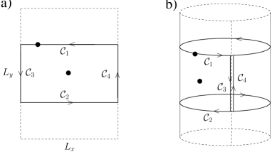
Figure 1: The “special” braiding path. This path makes use only of the asymptotic form of the two hole coherent state Eq. (27). a) The torus is represented as rectangular strip with periodic boundary conditions. b) Same as a) with two opposite ends of the strip in a) glued together. The two quasi-holes are represented as solid black dots.

As it turns out, the above difficulty can be overcome in two different ways. The complete solution to the problem makes use of the duality discussed earlier, and will be treated in the next section. However, this approach may obscure the physical origin of the abelian fractional statistics, which we hinted above is the simple shift of CDW ground state patterns surrounding each domain wall. To demonstrate this, we will first give a simplified treatment that makes the underlying physics quite transparent. To do so, we first restrict ourselves to the special class of braiding paths shown in Fig. (1), where one particle fully encircles the other. These paths contain two pieces ${\cal C}_{1}$ and ${\cal C}_{2}$ where one particle fully traverses one hole of the torus, in a regime where $|h_{1y}-h_{2y}|\gg 1$ holds and Eq. (27) is valid. The remaining parts ${\cal C}_{3}$ and ${\cal C}_{4}$ of the path cancel in the calculation of the Berry phase $\gamma$. After a simple calculation, using Eqs. (IV.2), (27), the latter can then be expressed as:

$$\gamma =-i\int_{{\cal C}_{1}+{\cal C}_{2}}d{\bf l}\cdot\langle\psi_{c}(h_{1},h_{2})|\nabla_{h_{1}}|\psi_{c}(h_{1},h_{2})\rangle$$ (29)

$$=\frac{-1}{m}\int_{{\cal C}_{1}}d{\bf l}{\bf A}_{-}(h_{1})+\frac{-1}{m}\int_{{\cal C}_{2}}d{\bf l}{\bf A}_{+}(h_{1})$$

$$=\frac{-1}{m}\int_{{\cal C}_{1}+{\cal C}_{2}}d{\bf l}{\bf A}_{-}(h_{1})+\frac{-1}{m}\int_{{\cal C}_{2}}d{\bf l}{\bf\,}\kappa\hat{e}_{x}$$

$$=\frac{-1}{m}\times\,\Phi\,+\frac{2\pi}{m}$$

In here, $\Phi$ is the magnetic flux through the area encircled by the closed path in Fig. (1a), and we used ${\bf A}_{+}={\bf A}_{-}+\kappa\hat{e}_{x}$ in the third line. Eq. (29) is the correct resultasw for two quasi-holes in a $\nu=1/m$ liquid. It is now apparent that the abelian statistics described by the term $2\pi/m$ have their root in the relative displacement of a ground state CDW pattern in the presence of a domain wall, since this is the cause for the difference between ${\bf A}_{-}$ and ${\bf A}_{+}$. We can easily generalize this result to the elementary excitations in hierarchy states. As shown in Ref. karl1, , the thin torus limit of a $\nu=p/(mp+1)$ state in the Jain hierarchyJain consists of unit cells of the form $C=(10_{m-1})_{p-1}10_{m}$, where a subscript denotes repetition of the building block it is attached to. In the same notation, the expression for a Laughlin state such as Eq. (3) would be $C=10_{m-1}$. Note that for Jain states, $m$ is even for fermions, as opposed to our convention for Laughlin states. An elementary excitation of charge $-e/{\mathfrak{q}}$, where ${\mathfrak{q}}\equiv mp+1$, corresponds to a domain wall defect in the thin torus limit where one of the shorter blocks $10_{m-1}$ is removed. In this limit, a state with two domain walls separated by a number of unit cells would read:

$$\dotsc\text{CCC}(10_{m-1})_{p-2}10_{m}\text{CCCCC}(10_{m-1})_{p-2}10_{m}\text{CCC}\dotsc$$ (30)

We may now postulate that for a state of two localized charge $-e/{\mathfrak{q}}$ excitations, an expression analogous to Eq. (27) holds. However, two important modifications apply. First, the definition of $b_{c,q}$ in Eq. (21) should be properly adjusted to refer to the position of a domain wall in the Jain state, i.e. $b_{c,q}=q{\mathfrak{q}}+c+\delta$.note Second, it is apparent from Eq. (30) that the shift between the CDW patterns surrounding a domain wall is now $\Delta c=-m$ rather than $\Delta c=+1$, since at each domain wall one $10_{m-1}$ block of length $m$ is removed. Then a calculation analogous to that in Eq. (29) yields

$$2\theta =2\pi\frac{\Delta c}{{\mathfrak{q}}}$$

for the statistical part of the Berry phase, with $\Delta c=-m$ in this case. In fact, the arguments leading to Eq. (V) can be expected to be valid beyond the Jain hierarchy. That is, whenever the domain wall picture for an elementary charge $-e/{\mathfrak{q}}$ excitation is known in an abelian quantum Hall state, we expect that its statistical angle $\theta$ satisfies Eq. (V). Here $\Delta c$ is the shift between CDW patterns caused by the domain wall, and the filling factor is $\nu=p/{\mathfrak{q}}$ with $p$ and ${\mathfrak{q}}$ coprime. This agrees with the general result obtained in Ref. wpsu, . Indeed, for a charge $-e/{\mathfrak{q}}$ excitation, the Schrieffer-Su counting argument implies a relation of the form

$$\Delta c\,p-n{\mathfrak{q}}=1\;,$$ (32)

where $n$ is an integer.note1 With this, the result in Ref. wpsu, then implies

$$2\theta=2\pi\frac{\Delta c^{2}p}{{\mathfrak{q}}}\;\mod\;2\pi\;.$$ (33)

However, using Eq. (32) again, Eqs. (V) and (33) agree modulo $2\pi$. Note that for a charge $+e/{\mathfrak{q}}$ defect, Eq. (V) requires an additional minus sign. This corresponds to the fact that Eq. (21) should be replaced by its complex conjugate in this case. Since $\Delta c$ will also change sign, the statistical phase remains the same.

We should, however, be careful not to apply Eq. (V) to excitations that can be regarded as composites of more elementary excitations, such as charge $p/{\mathfrak{q}}$ Laughlin quasi-particles in hierarchy states with $p>1$.note2 For composite particles, more complicated expressions are generally needed to properly localize these particles in both $x$ and $y$. Once the statistical phases for the most elementary excitations are known, those of composite particles can be calculated from the well known composition rule.yswu1 ; yswu2 We note, however, that we have so far determined $\theta$ only modulo $\pi$. This is so because we have not carried out a single exchange of two particles. We will remedy this fact in the following section. Although we will focus on Laughlin states from now on for simplicity, we believe that it is not difficult to generalize the following discussion to elementary excitations in arbitrary abelian states.

VI The Berry phase of exchange: Duality

While the above discussion offers most straight-forward insights into the nature of abelian statistics from our 1d point of view, it has certain limitations which we now wish to overcome. One limitation is the fact that the approach in the preceding section cannot be generalized to the non-abelian case even in principle. This is because the paths ${\cal C}_{3}$ and ${\cal C}_{4}$ in Fig. (1) are separated by paths ${\cal C}_{1}$ and ${\cal C}_{2}$, hence they need not cancel in the non-abelian case, where all these paths will be represented by non-commuting matrices. Also, since braiding statistics are a topological phenomenon, it is desirable to demonstrate their validity for more general paths, rather than the special ones considered so far. We will now show how this is achieved using duality.

The key idea is that in addition to Eq. (IV.2), one could write down a similar expansion for a two-hole state in terms of adiabatically evolved domain walls from the limit $L_{y}\rightarrow 0$ ($L_{x}\rightarrow\infty$)

$$|\psi_{\bar{c}}(h_{1},h_{2})\rangle=\sum_{q_{1}<q_{2}}\,\bar{\varphi}^{\ast}_{\bar{c},q_{1},q_{2}}(h_{1},h_{2})\,\hat{S}(L_{x},\infty)\bigl{.}\overline{\bigl{|}{\bar{c}},q_{1},q_{2}\bigr{.}}\bigr{>}.$$

Similar as before, $\bar{c}$ is the CM index for the CDW in the $L_{x}\rightarrow\infty$ limit. By going through steps similar to those leading to Eq. (27), we can give an asymptotic form for $\bar{\varphi}_{\bar{c},q_{1},q_{2}}$ which is valid when $\bar{\kappa}(q_{2}-q_{1})\gg 1$

$$\bar{\varphi}_{\bar{c},q_{1},q_{2}}(h_{1},h_{2})\simeq{\cal N}^{2}_{\bar{\varphi}}\,\bar{\varphi}_{\bar{c},q_{1}}(h^{<})\bar{\varphi}_{\bar{c}+1,q_{2}}(h^{>}),$$ (35)

where

$$\bar{\varphi}_{\bar{c},q}(h)=e^{-iq(h_{y}\bar{\kappa}+\pi)-\frac{1}{2m}(h_{x}-\bar{\kappa}b_{\bar{c},q})^{2}},$$ (36)

and $(h^{<},h^{>})$ equals $(h_{1},h_{2})$ for $h_{1x}<h_{2x}$, and $(h_{2},h_{1})$ otherwise. Eq. (35) is valid for $\bar{\kappa}(q_{2}-q_{1})\gg 1$, and hence can be used in Eq. (VI) for $|h_{1x}-h_{2x}|\gg 1$.

In calculating the Berry phase for the exchange of two holes, we can now employ the following strategy. We start with two holes in the state $|\psi_{c}(h_{1},h_{2})\rangle$, having large $|h_{1y}-h_{2y}|$. Initially, $h_{1x}=h_{2x}$ is assumed. Keeping $h_{2}$ fixed, we move $h_{1}$ around $h_{2}$ in a counter-clockwise manner, dividing the contour ${\cal C}$ into three parts (Fig. (2)). Along ${\cal C}_{1}$, a contribution $\gamma_{1}$ to the Berry phase can be calculated using Eqs. (IV.2),(27), since $h_{1y}-h_{2y}\gg 1$ holds. Simple calculation gives

$$\gamma_{1} =-i\int_{{\cal C}_{1}}d{\bf l}\cdot\langle\psi_{c}(h_{1},h_{2})|\nabla_{h_{1}}|\psi_{c}(h_{1},h_{2})\rangle$$ (37)

$$=\frac{-1}{m}\int_{{\cal C}_{1}}d{\bf l}\cdot{\bf A}_{+}(h_{1}),$$

where ${\bf A}_{+}$ is given in Eq. (28). At the point labeled 2, we can then switch to Eqs.(VI) and (35). However before doing so we need to write $|\psi_{c}(h_{1},h_{2})\rangle$ as linear combinations of $|\psi_{\bar{c}}(h_{1},h_{2})\rangle$ as follows

$$|\psi_{c}(h_{1},h_{2})\rangle\,\bigr{|}_{2}=\sum_{\bar{c}}u_{c\bar{c}}~{}~{}|\psi_{\bar{c}}(h_{1},h_{2})\rangle\,\bigr{|}_{2}$$ (38)

Along ${\cal C}_{2}$, the expressions (VI),(35) can be used to yield

$$\gamma_{2}(\bar{c}) =-i\int_{{\cal C}_{2}}d{\bf l}\cdot\langle\psi_{\bar{c}}(h_{1},h_{2})|\nabla_{h_{1}}|\psi_{\bar{c}}(h_{1},h_{2})\rangle$$ (39)

$$=\frac{-1}{m}\int_{{\cal C}_{2}}d{\bf l}\cdot{\bf B}_{-}(h_{1}),$$

where

$${\bf B}_{-}(z)=(0,x-\bar{\kappa}\bar{c}-\bar{\kappa}{m+1\over 2})$$

$${\bf B}_{+}(z)=(0,x-\bar{\kappa}(\bar{c}+1)-\bar{\kappa}{m+1\over 2}).$$ (40)

Since our state was originally in the sector labeled $c$, we expect that this remains true even after the adiabatic evolution along ${\cal C}_{2}$. At point 3 we must then have

$$\sum_{\bar{c}}\bigl{.}u_{c\bar{c}}\,e^{i\gamma_{2}(\bar{c})}\left|\psi_{\bar{c}}(h_{1},h_{2})\right>\,\bigr{|}_{3}=e^{i\gamma_{2}}\bigl{.}\left|\psi_{c}(h_{1},h_{2})\right>\,\bigr{|}_{3}.$$ (41)

We note that the validity of a relation of this form is not trivial, since the constants $u_{c\bar{c}}$ appearing in it are the same as those defined at point 2 in Eq. (38). However, Eq. (38) is necessarily true if the evolution along ${\cal C}_{2}$ does not affect the original sector of the state, which has the label $c$. For abelian statistics this is what one expects, and we will verify the validity of Eq. (41) within our framework below (see Appendix A, Eqs. (71)-(73) ).

Finally, for the contribution ${\cal C}_{3}$ to the Berry phase, we may again use Eqs. (IV.2),(27). Since now $h_{1}=h^{-}$, the Berry connection is given by $\frac{-1}{m}{\bf A}_{-}(h_{1})$, thus

$$\gamma_{3} =-i\int_{{\cal C}_{3}}d{\bf l}\cdot\langle\psi_{c}(h_{1},h_{2})|\nabla_{h_{1}}|\psi_{c}(h_{1},h_{2})\rangle$$ (42)

$$=\frac{-1}{m}\int_{{\cal C}_{1}}d{\bf l}\cdot{\bf A}_{-}(h_{1}).$$

As a last step, we displace both holes vertically until they have exchanged their original positions, yet this does not contribute to the Berry phase. Note that, as opposed to the preceding section, our current path ${\cal C}$ describes a true exchange of two particles, not the full encircling of one particle by the other. The total Berry phase for this path is given by

$$\gamma=\gamma_{1}\!+\!\gamma_{2}\!+\!\gamma_{3}.$$ (43)

By overlapping Eq. (38) with $|\psi_{\bar{c}}(h_{1},h_{2})\rangle|_{2}$ and Eq.(41) with $|\psi_{\bar{c}}(h_{1},h_{2})\rangle|_{3}$ we obtain

$$\gamma_{2}=\gamma_{2}(\bar{c})+\lambda(\bar{c})$$

$$\lambda(\bar{c})\!=\!-i\ln\left({\left<\psi_{\bar{c}}|\psi_{c}\right>_{2}\over\!\left<\psi_{\bar{c}}|\psi_{c}\right>_{3}}\right).$$ (44)

Note that by Eq. (41), the above result for $\gamma_{2}$ must be independent of the choice for $\bar{c}$, so long as the overlaps entering this expression do not vanish. Hence the dependence on $\bar{c}$ will cancel in the expression for $\gamma_{2}$. Writing ${\bf B}_{-}={\bf A}_{+}+\nabla f_{1}$, ${\bf A}_{-}={\bf A}_{+}+\nabla f_{2}$, where $f_{1}(z)=xy\!-\!\kappa(c+{m+1\over 2}\!+\!1)x\!-\!\bar{\kappa}(\bar{c}+{m+1\over 2})y$, $f_{2}(z)=-\kappa x$, the final result for the Berry phase can be expressed as

$$\gamma =\gamma_{1}\!+\!\gamma_{2}\!+\!\gamma_{3}=-\frac{1}{m}\int_{\cal C}\,dh_{1}\,{\bf A}_{+}(h_{1})$$ (45)

$$+[\lambda(\bar{c})+\frac{1}{m}(f_{1}|_{\begin{subarray}{c}\\ 2\end{subarray}}-f_{1}|_{\begin{subarray}{c}\\ 3\end{subarray}}+f_{2}|_{\begin{subarray}{c}\\ 3\end{subarray}}-f_{2}|_{\begin{subarray}{c}\\ 4\end{subarray}})]$$

where $f|_{p}$ denotes the value of $f$ at point $p$.

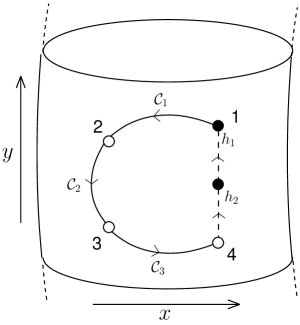
Figure 2: Two quasi-holes (solid black) on a torus are exchanged along a path ${\cal C}$. The position of one particle is kept at $h_{2}$, while the other at $h_{1}$ traces the shown path. The path is divided in to parts ${\cal C}_{1}$, ${\cal C}_{2}$, ${\cal C}_{3}$, separated by points labeled $1$-$4$.

The first term in Eq. (45) is again equal to

$$\frac{-1}{m}\int_{\cal C}\,dh_{1}\,{\bf A}_{+}(h_{1})=\frac{-1}{m}\times\,\Phi$$ (46)

Here $\Phi$ denotes the magnetic flux enclosed by the exchange path consisting of the pieces ${\cal C}_{1}+{\cal C}_{2}+{\cal C}_{3}$ and the final vertical step discussed above. This is the Aharonov-Bohm component of the Berry phase. Our final task is thus to calculate $[\lambda(\bar{c})+\frac{1}{m}(f_{1}|_{\begin{subarray}{c}\\ 2\end{subarray}}-f_{1}|_{\begin{subarray}{c}\\ 3\end{subarray}}+f_{2}|_{\begin{subarray}{c}\\ 3\end{subarray}}-f_{2}|_{\begin{subarray}{c}\\ 4\end{subarray}})]$ using Eq. (VI). This in turn requires us to compute overlaps of the form $\left<\psi_{c}|\psi_{\bar{c}}\right>$ from Eqs. (IV.2),(VI).

To achieve this, we need to compute the overlap between $\hat{S}(L_{x},\infty)\,\bigr{.}\overline{\left|\bar{c},p_{1},p_{2}\right.}\bigr{>}$ and $\hat{S}(L_{x},0)|c,q_{1},q_{2}\rangle$. The details of the calculation are carried out in Appendix A. Two cases need to be distinguished. In the first case, the particles are either bosons ($m$ even) of arbitrary particle number $N$, or are fermions of odd total particle number ($m$, $N$ both odd). The second case is that of fermions with even particle number ($m$ odd, $N$ even). The latter case is different by means of the special role played by the fermion negative sign in translations, and needs to be treated separately. This distinction is at the heart of the “odd denominator rule” for fermion quantized Hall states. How this rule manifests itself in full generality within our 1d framework will be discussed elsewhere.seidel3 For brevity, we will write down here the result for the first case (in which $m(N-1)$ is even):

$$\begin{split}&\left<c,q_{1},q_{2}\left|\hat{S}^{\dagger}(L_{x},0)\hat{S}(L_{x},\infty)\,\right.\overline{\Bigl{|}\bar{c},p_{1},p_{2}\Bigr{.}}\right>=\cfrac{\sqrt{m}}{L}\times\\ &\Big{(}\exp\{\frac{i\pi}{m}((2-\frac{2}{L})b_{\bar{c},p_{1}}b_{c,q_{1}}+mN(b_{\bar{c},p_{1}}+b_{c,q_{1}})+b_{\bar{c}\!+\!1,p_{2}}\\ &+b_{c\!+\!1,q_{2}}-\frac{2}{L}b_{\bar{c}\!+\!1,p_{2}}b_{c\!+\!1,q_{2}})\}+\exp\{\frac{i\pi}{m}((2\!-\!\frac{2}{L})b_{\bar{c},p_{1}}b_{c\!+\!1,q_{2}}\\ &+mN(b_{\bar{c},p_{1}}\!+\!b_{c\!+\!1,q_{2}})+b_{c,q_{1}}\!-\!b_{\bar{c}\!+\!1,p_{2}}\!-\!\frac{2}{L}b_{\bar{c}\!+\!1,p_{2}}b_{c,q_{1}}\!+\!L)\}\Big{)}\,,\end{split}$$ (47)

where $b_{c,q}$ is defined below Eq. (21). Eq. (47) is derived in Appendix A, along with the corresponding result for the case $m(N-1)$ odd. Again, Eq. (47) holds only for $\kappa(b_{c,q_{2}}-b_{c,q_{1}})\gg 1$, $\bar{\kappa}(b_{\bar{c},p_{2}}-b_{\bar{c},p_{1}})\gg 1$. These conditions are satisfied for the values of $q_{1},q_{2},p_{1},p_{2}$ that give rise to the exponentially dominant terms in the overlap $\left<\psi_{c}(h_{1},h_{2})|\psi_{\bar{c}}(h_{1},h_{2})\right>$ at points 2 and 3, because at these points $|h_{1x}-h_{2x}|$ and $|h_{1y}-h_{2y}|$ are both large. This overlap can now be calculated by putting together Eqs. (IV.2), (27), (VI)-(36) and (47). In the dominant region of the resulting sum over $q_{i},p_{i}$ where the Gaussian factors are near their peak, the first (second) exponential in Eq. (47) gives rise to a smoothly varying phase as a function of the $q_{i},p_{i}$ at point 3 (point 2). This term then dominates the sum and can be converted into a Gaussian integral. This way, one finds the quantities $u_{c\bar{c}}$ defined via Eq. (38) at point 2. The explicit expression is given in the Appendix, Eq. (71). It is readily seen that these quantities form a unitary matrix, as is required. At point 3 the same procedure shows that a relation of the form Eq. (41) is indeed satisfied, involving the same matrix $u_{c\bar{c}}$ obtained at point 2, and hence the abelian phase $\gamma_{2}$ is well defined (c.f. Appendix A, Eq. (A)). The final result for the statistical phase is then:

$$[\lambda(\bar{c})+\frac{1}{m}(f_{1}|_{\begin{subarray}{c}\\ 2\end{subarray}}-f_{1}|_{\begin{subarray}{c}\\ 3\end{subarray}}+f_{2}|_{\begin{subarray}{c}\\ 3\end{subarray}}-f_{2}|_{\begin{subarray}{c}\\ 4\end{subarray}})]={\pi\over m}\,(\text{mod}\,2\pi)\,.$$ (48)

This, together with Eqs. (45), (46) is exactly the result expected for an exchange of two Laughlin quasi-holes.

VII Discussion

In the preceding two sections we have shown how the braiding properties of Laughlin quasi-holes emerge in a Hilbert space made up of one-dimensional domain walls. The notion of “braiding” in these systems arises by considering coherent states which describe domain walls having a narrow distribution both in position space as well as in momentum space of the 1d system. From the 1d point of view, quasi-holes are thus objects localized in the phase space of the system. Since the phase space is two dimensional, the notion of braiding is well defined, and this phase space is identified with the original 2d torus of the quantum Hall system. In this manner, even from a 1d viewpoint one can recover the well-known fact that Laughlin quasi-holes behave as fractionally charged anyons in a background magnetic field, as first derived by Arovas, Schrieffer and Wilczek (ASW).asw

The fact that it is possible to rephrase the physics of fractional quantum Hall systems in this 1d language reflects the 1d structure of Landau levels, and the related non-commutative geometry of the physics in a strong magnetic field. However, a brute force expansion of wave-functions in the Landau level “lattice” basis is not very feasible from an analytic point of view. It is only due to the remarkable adiabatic continuity between quantum Hall states and simple 1d CDW patterns in the thin torus limit that a simple 1d language for quantum Hall states can be obtained. In earlier works, we had discussed how the intricate quantum numbers of quantum Hall states may be inferred from these simple CDW patterns, such as the characteristic degeneracies and the fractional charge of excitations. However, the thin torus limit as a starting point seemed to contain no information about a dynamical principle that would allow one to understand properties such as braiding statistics. In this work we showed how the limiting CDW patterns organize the space of quasi-hole like excitation such that, when combined with the duality principle on the torus, the statistics of Laughlin-quasi holes can be derived. While the underlying calculation is less straightforward than the standard ASW procedure, it has a number of attractive features. Unlike in the ASW treatment, it is quite apparent in our method that corrections to the Berry phase Eq. (48) will die off exponentially with the radius of the exchange path. In the traditional approach this fact had been obscured by the finite extent of the quasi holes.asw More importantly, the ASW treatment makes use of the very special product structure of Laughlin-type wavefunctions. Therefore it cannot be carried over to more complicated cases in principle. While we have not yet shown that our method makes the calculation of non-abelian statistic a workable task, we believe that the general structure of our approach does carry over to the non-abelian case. To be specific, we point out that the local Berry connections which arise in the basis of adiabatically continued domain-wall states are locally trivial, describing a charge $-e/m$ particle interacting with a constant magnetic background field (Eqs. (28), (40)). We conjecture that this feature also holds in the non-abelian case. That is, we conjecture that in the basis of adiabatically continued domain wall states, the local Berry connection will be diagonal along each path segment in Fig. (2). The information about non-abelian statistics would then be entirely contained in the transition functions describing the change between the two mutually dual sets of basis wavefunctions at points 2 and 3, which generalize Eqs. (38) and (41) of this paper to the non-abelian case. This may considerably reduce the task of deriving non-abelian statistics directly from wavefunctions. We reserve a detailed study of this conjecture for future work.

VIII Conclusion

To conclude we have, in previous works, established that the fractional charge of the abelian and non-abelian quasiparticles can be understood as the fractional charge carried by the solitons in appropriate one dimensional CDW systems (Refs. seidel1, ; seidel2, , c.f. also Refs. karl1, ; karl2, ). In this paper we show that the fractional statistics of the abelian quasiparticles can also be understood in this language. The bottom line is that the Laughlin quasiparticle state is the coherent state of the one-dimensional solitons. We have explicitly calculated the expansion coefficient of such coherent states in terms of the position eigenstates of the solitons. These expansions were obtained by making contact with Laughlin wavefunctions. However, their simple structure seems to follow naturally from the symmetries of the problem, as well as the non-commutative geometry of the physics in a strong magnetic field. The latter leads to the identification of the two-dimensional surface of a quantum Hall torus with the position-momentum phase space of a one-dimensional (lattice) system. The role of localized Laughlin quasi-particles is then naturally identified with that of coherent states formed by domain-wall type excitations in the 1d picture. Based on this approach we were able to give a new derivation for the statistics of Laughlin quasi-particles. This approach also makes use of the inherent duality of the 1d formalism, and does not appear to be as closely tied to the specific structure of Laughlin wavefunctions when compared to the traditional approach. We are hopeful that the formalism presented here will offer ways to calculate the braiding statistics for non-abelian states, where the traditional many-body wavefunctions are far more complicated.mooreread ; readrezayi

Appendix A Relation between dual representations and other details

In this Appendix we derive the relation between states that are obtained by the adiabatic evolution of two-domain-wall states from opposite thin torus limits, i. e. $L_{x}\rightarrow 0$ and $L_{y}\rightarrow 0$, respectively. This relation is needed to calculate the overlap in Eq. (47). We first solve the analogous problem for single hole domain wall states on a torus with $L=mN+1$ flux quanta. Thus we seek an expression of the form

$$\hat{S}(L_{x},\infty)\overline{|\bar{c},p}\rangle=\sum_{c,q}u(\bar{c},p|c,q)\hat{S}(L_{x},0)\bigl{|}{c,q}\bigr{>}$$ (49)

Note that the sum on the right hand side is not restricted to a single $c$-sector. Hence to ease the notation and the expressions that follow, we will now label states by the domain-wall positions

$$b\equiv b_{c,q}=mq+c+\frac{1}{2}(m+1)$$ (50)

and

$$a\equiv b_{\bar{c},p}=mp+\bar{c}+\frac{1}{2}(m+1)$$ (51)

respectively. Recall that $\bar{\kappa}a$ and $\kappa b$ are just the $x-$ and $y-$positions of a domain-wall in the states

$$\overline{|a}\rangle\equiv\overline{|\bar{c},p}\rangle\;,\;|b\rangle\equiv|c,q\rangle$$ (52)

respectively. We shall also use the abbreviations

$$\hat{S}\equiv\hat{S}(L_{x},0)\;,\;\;\hat{\bar{S}}\equiv\hat{S}(L_{x},\infty)$$ (53)

in the following. With the notation Eqs. (50), (53) we can rewrite Eq. (49) in the more compact form

$$\hat{\bar{S}}\overline{|a}\rangle=\sum_{b}u(a|b)\,\hat{S}\bigl{|}{b}\bigr{>}\;.$$ (54)

Note that from Eq. (50), $a$ and $b$ are both integer for $m$ odd, and half-odd integer for $m$ even. The sum in Eq. (54) thus goes over all integer or half-odd integer values in the interval $[0,L)$, depending on $m$.

We now observe that $\hat{\bar{S}}{\bigl{.}\overline{\bigl{|}a\bigr{.}}\bigr{>}}$ is an eigenstate of $T_{y}$ with eigenvalue $\exp(-ik)$, $k=-\frac{2\pi}{Lm}a+\pi(N+\frac{2}{m}a)$. This implies that $\hat{\bar{S}}{\bigl{.}\overline{\bigl{|}a\bigr{.}}\bigr{>}}$ has the form of a plane wave in terms of the states $\hat{S}\bigl{|}{b}\bigr{>}$,i.e.

$$\hat{\bar{S}}{\bigl{.}\overline{\bigl{|}a\bigr{.}}\bigr{>}}\,\propto\frac{1}{\sqrt{L}}\sum_{b}e^{ikb}\hat{S}\bigl{|}{b}\bigr{>}.$$ (55)

For the time being, we restrict ourselves to the cases where the underlying particles are either bosons ($m$ even, $N$ arbitrary), or fermions with an odd total number of particles ($m$, $N$ both odd). In both these cases the domain wall states transform straightforwardly under translations,

$$T_{y}|{b}\bigr{>}=\left\{\begin{array}[]{ll}|{b+1}\bigr{>}&\text{for $b+1<L$}\\ |{b+1-L}\bigr{>}&\text{otherwise}\end{array}\right.$$ (58)

The situation is slightly more complicated for fermions when the particle number $N$ is even. This is so because then an additional minus sign arises whenever an electron in the state $|b\rangle$ is translated across the boundary between the orbital labeled $L-1$ and the orbital labeled $0$. Said succinctly, we distinguish the following two cases:

$$\begin{split}\text{case~{}~{}i)}&\quad m(N-1)\;\;\text{even}\\ \text{case ii)}&\quad m(N-1)\;\;\text{odd}\end{split}$$ (59)

where we leave it understood that the underlying particles are fermions if $m$ is even, and bosons if $m$ is odd. We first consider case i) where Eq. (58) holds, and deal with case ii) later. From Eq. (58) it is easily verified that the right hand side of Eq. (55) has the correct $T_{y}$ eigenvalue, since $T_{y}$ commutes with the evolution operator $\hat{S}$. The expression Eq. (55) is, however, not complete yet. We must still choose the overall phase of the right hand side in a consistent manner. The correct phase as a function of $a$ can be determined from the requirement that $T_{x}\hat{\bar{S}}{\bigl{.}\overline{\bigl{|}a\bigr{.}}\bigr{>}}=\hat{\bar{S}}{\bigl{.}\overline{\bigl{|}a\!+\!1\bigr{.}}\bigr{>}}$. Alternatively, using duality it can be shown that $u(a|b)$ must be symmetric in $a$ and $b$, i.e. $u(a|b)=u(b|a)$. Both requirements yield that the overall phase factor in Eq. (55) must be $\exp(i\pi Na)$. Altogether, this results in

$${\bigl{<}b\bigr{|}}\hat{S}^{\dagger}\hat{\bar{S}}{\bigl{.}\overline{\bigl{|}a\bigr{.}}\bigr{>}}=u(a|b)$$

$$=\frac{1}{\sqrt{L}}\exp\{\frac{i\pi}{m}((2-\frac{2}{L})ab+mN(a+b))\}$$ (60)

We now turn to the actual two-hole problem on a torus with $L=mN+2$ flux quanta. Let us seek an expansion for $\hat{\bar{S}}{\bigl{.}\overline{\bigl{|}a_{1},a_{2}\bigr{.}}\bigr{>}}\equiv\hat{\bar{S}}{\bigl{.}\overline{\bigl{|}\bar{c},p_{1},p_{2}\bigr{.}}\bigr{>}}$ in terms of the states $\hat{S}{\bigl{.}{\bigl{|}b_{1},b_{2}\bigr{.}}\bigr{>}}\equiv\hat{S}{\bigl{.}{\bigl{|}c,q_{1},q_{2}\bigr{.}}\bigr{>}}$,

$$\hat{\bar{S}}{\bigl{.}\overline{\bigl{|}a_{1},a_{2}\bigr{.}}\bigr{>}}=\sideset{}{{}^{\prime}}{\sum}_{b_{1}<b_{2}}u(a_{1},a_{2}|b_{1},b_{2})\hat{S}{\bigl{.}{\bigl{|}b_{1},b_{2}\bigr{.}}\bigr{>}}.$$ (61)

Again, $m$ determines whether the sum goes over integer or half-odd integer values. In addition, the following constraints apply:

$$0\leq a_{1}<a_{2}<L\,, \;0\leq b_{1}<b_{2}<L$$

$$a_{2}-a_{1}\equiv 1\mod m\,, \;b_{2}-b_{1}\equiv 1\mod m$$ (62)

The second line expresses the fact that the second domain-wall is inserted into a CDW pattern which is shifted by one lattice site relative to the pattern surrounding the first domain wall. The prime on the sum in Eq. (61) denotes that the constraint Eq. (62) is enforced.

As in deriving Eq. (27), we are facing the problem that the matrix elements $u(a_{1},a_{2}|b_{1},b_{2})$ are not entirely determined by translational symmetry alone. To make progress, we first of all assume that the domain wall positions $a_{1}$ and $a_{2}$ are well separated, i.e. $\bar{\kappa}(a_{2}-a_{1})\gg 1$, such that the “dressing” of each domain wall by the operator $\hat{\bar{S}}$ will be unaffected by the presence of the other domain wall. The two defects are then independent. When the separation of the $\kappa(b_{2}-b_{1})$ in the expansion Eq. (61) is also large, we expect that the expression in Eq. (61) should be of a plane-wave form analogous to Eq. (55) in both variables $b_{1}$ and $b_{2}$. We thus write down an ansatz of the form

$$u(a_{1},a_{2}|b_{1},b_{2})\simeq{\cal N}_{u}e^{\beta(a_{1},a_{2})}\!\!\left(e^{ik_{1}b_{1}+ik_{2}b_{2}}\!+\!e^{i\lambda}e^{ik_{1}b_{2}+ik_{2}b_{1}}\right)$$

for $\kappa(b_{2}-b_{1})\gg 1$, $\bar{\kappa}(a_{2}-a_{1})\gg 1$, where we must now determine the parameters $\beta$, $k_{1}$, $k_{2}$, $\lambda$ as a function of $a_{1}$, $a_{2}$, $b_{1}$, $b_{2}$. We first use translational symmetry. One finds that $\hat{\bar{S}}{\bigl{.}\overline{\bigl{|}a_{1},a_{2}\bigr{.}}\bigr{>}}$ is an eigenstate of $T_{y}$ with eigenvalue $\exp(-iK)$, where

$$K=\frac{\pi}{m}(-\frac{2}{L}(a_{1}+a_{2})+Nm+2a_{1}+\eta)\mod 2\pi\,.\,$$ (64)

In the above, the constant $\eta\equiv 1$ comes from the constraint $a_{2}-a_{1}\equiv 1\mod m$ in Eq. (62). It is useful to introduce this dummy variable, since one would naively expect that $a_{1}$ and $a_{2}$ should enter expressions such as Eq. (64) more symmetrically. Due to the form of the constraint however, the expression is truly symmetric only under the exchange $a_{1}\leftrightarrow a_{2}$ and the simultaneous substitution $\eta\rightarrow-\eta$. Although this symmetry is not immediately obvious in equation Eq. (64), it is easily checked that it is satisfied (modulo $2\pi$). Similar statements hold for some of the expressions that will follow, hence $\eta$ is best retained as a variable for easy consistency checks. Furthermore, we also note that $\exp(iKL)=1$ holds as required by periodic boundary conditions. The requirement that the right hand side of Eq. (61) must also be a $T_{y}$ eigenket with eigenvalue $\exp(-iK)$ leads to the following conditions:

$$k_{1}+k_{2}=K\mod 2\pi$$ (65)

$$\lambda=-k_{1}L=k_{2}L\mod 2\pi$$ (66)

where in the last line, it was used that $T_{y}\hat{S}{\bigl{.}{\bigl{|}b_{1},b_{2}\bigr{.}}\bigr{>}}=\hat{S}{\bigl{.}{\bigl{|}b_{2}\!+\!1\!-\!L,b_{1}\!+\!1\bigr{.}}\bigr{>}}$ holds when $b_{2}+1>L$. We now determine how the phase factors $e^{ib_{j}k_{j^{\prime}}}$ in Eq. (A) must change when a domain wall undergoes a local move. For this we first need to make precise what a local move is. We stress again that it is not possible for any domain wall to change its position $b_{i}$ by an amount smaller than $\pm m$ without shifting the entire fluid, i.e. without changing the low energy sector $c$. This is evident from Eqs. (50). Thus it is clear that a change of any domain-wall position by an amount $\Delta b<m$ is not a “local” move, but affects an infinite number of degrees of freedom. In contrast, a domain-wall move by $\Delta b=\pm m$ only requires the hopping of a single electron in the thin torus limit. Even for the “dressed” domain walls at finite circumference, we expect that a local operator (such as the local charge density operator) will be able to generate matrix elements only between states $\hat{S}{\bigl{.}{\bigl{|}b_{1},b_{2}\bigr{.}}\bigr{>}}$ whose domain wall positions $b_{1}$ or $b_{2}$ differ by a few integer multiples of $m$. Hence it is the change of the phase factors $e^{ib_{j}k_{j^{\prime}}}$ in Eq. (A) under a change of $b_{j}$ by $\pm m$ that will determine physical properties like the charge density profile of the state Eq. (61). Let us consider the single hole case, Eq. (55). We note that in a state describing a hole localized at $h_{x}\equiv\bar{\kappa}a$, the phase of $\hat{S}\bigl{|}{b}\bigr{>}$ always changes by the following amount when $b\rightarrow b+m$:

$$e^{ikm} =e^{-2\pi ia/L+i\pi(Nm+2a)}$$ (67)

$$=-e^{-2\pi ia/L}=-e^{-i\kappa h_{x}},$$

where we have used that $Nm+2a$ is always odd in case i) (Eq. (59)) which we are considering here. Incidentally, the same change of phase under $b\rightarrow b+m$ as that shown in Eq. (67) can already be observed in the single hole coherent state Eqs. (17),(21), and more importantly so in the two-hole coherent state Eqs. (26),(27). It is thus quite clear that we must also have

$$e^{ik_{1,2}m}=-e^{-2\pi ia_{1,2}/L}$$ (68)

in Eq. (A), in order for the state Eq. (61) to describe two dressed domain walls at $x$-positions $\bar{\kappa}a_{1,2}$. The conditions Eqs. (64),(68) are satisfied by the following choice of the momenta $k_{1}$, $k_{2}$,

$$\begin{split}k_{1}&=\frac{\pi}{m}(-\frac{2}{L}a_{1}+2a_{1}+Nm)\\ k_{2}&=\frac{\pi}{m}(-\frac{2}{L}a_{2}+\eta)\;.\end{split}$$ (69)

Superficially, it looks like one could have made different choices for $k_{1}$, $k_{2}$ that also satisfy Eqs. (64),(68). However, using the constraint Eq. (62) it can be shown that all these choices give rise to the same state, up to a trivial overall phase. In general, one may let $k_{1}\rightarrow k_{1}\!+\!\Delta$, $k_{2}\rightarrow k_{2}\!-\!\Delta$, where $\Delta$ is an integer multiple of $2\pi/m$, without changing the state Eq. (61). In particular, the state Eq. (61) is invariant (up to a phase) when all indices $1$ and $2$ are exchanged in Eq. (69), and the substitution $\eta\rightarrow-\eta$ is made. Finally, we fix the overall phase of the state by choosing $\beta(a_{1},a_{2})$ in Eq. (A). Again we do this by requiring that the state Eq. (61) transforms properly under $T_{y}$ translations, i.e. $T_{y}\hat{\bar{S}}{\bigl{.}\overline{\bigl{|}a_{1},a_{2}\bigr{.}}\bigr{>}}=\hat{\bar{S}}{\bigl{.}\overline{\bigl{|}a_{1}+1,a_{2}+1\bigr{.}}\bigr{>}}$, and that the matrix element $u(a_{1},a_{2}|b_{1},b_{2})$ is symmetric under the simultaneous exchange $a_{1}\leftrightarrow b_{1}$, $a_{2}\leftrightarrow b_{2}$, as required by duality. This way one obtains

$$\beta(a_{1},a_{2})=\frac{\pi}{m}(Nm\,a_{1}+\eta\,a_{2}).$$ (70)

With this choice, the first term in Eq. (A) is manifestly symmetric under the exchange $a_{j}\leftrightarrow b_{j}$, and the second term can be shown to have this symmetry using again Eq. (62). Plugging Eqs. (70),(69), (66), and $\eta\equiv 1$ into Eq. (A) yields the matrix element $u(a_{1},a_{2}|b_{1},b_{2})$ displayed in Eq. (47). In writing Eq. (47), we also used that due to the asymptotic plane wave form of $u(a_{1},a_{2}|b_{1},b_{2})$, the normalization ${\cal N}_{u}$ must be equal to the square root of the number of terms in Eq. (A), at least to the leading order in $1/L$. This yields ${\cal N}_{u}\simeq\sqrt{m}/L$. Although this result does not enter our determination of the Berry phase, it is interesting to note that corrections to it are actually exponentially small. This can be shown from the requirement that the matrix formed by the quantities $u_{c\bar{c}}$ in Eq. (38) must be unitary, as we will see shortly. We had refrained from giving a detailed expression for these quantities in the main text for brevity. This expression will be given in the following. By carrying out the procedure described in Section VI at point 2 (Fig. (2)), one obtains:

$$u_{c\bar{c}} =\frac{L^{2}}{2m^{2}}{{\cal N}^{1}_{\varphi}{{\cal N}^{2}_{\varphi}}{{\cal N}_{u}}\exp\{-\frac{i}{m}[\pi mN(\bar{c}+c+m+2)}$$ (71)

$$+\pi m(\bar{c}+c+m)+\pi m+2\pi(c+\frac{m+1}{2})(\bar{c}+\frac{m+1}{2})$$

$$-\kappa(c+\frac{m+1}{2})(h_{1x}+h_{2x})-\bar{\kappa}(\bar{c}+\frac{m+1}{2})(h_{1y}+h_{2y})$$

$$-\kappa h_{1x}-\bar{\kappa}h_{2y}+h_{1x}h_{1y}+h_{2x}h_{2y}]\}$$

$$\equiv\langle\psi_{\bar{c}}(h_{1},h_{2})|\psi_{c}(h_{1},h_{2})\rangle\bigr{|}_{2}$$

It is easily seen that the above expression is proportional to a unitary matrix. Since we are interested in domain walls that are well separated in $x$ and $y$, one can determine the normalization constants ${\cal N}^{1}_{\varphi}=\kappa\sqrt{m/\pi}$ and ${\cal N}^{2}_{\varphi}=\bar{\kappa}\sqrt{m/\pi}$ from Eqs. (27) and (35) up to exponentially small corrections. The condition that $u_{c\bar{c}}$ is unitary then yields ${\cal N}_{u}=\sqrt{m}/L$, as anticipated. At point 3 one may calculate the overlap between the states $\psi_{c}$ and $\psi_{\bar{c}}$ using the same procedure. This defines the phase $\gamma_{2}$, as explained in Section VI. One finds:

$$\langle\psi_{\bar{c}}(h^{\prime}_{1},h_{2})|\psi_{c}(h^{\prime}_{1},h_{2})\rangle\bigr{|}_{3}=u_{c\bar{c}}|_{\begin{subarray}{c}\\ h_{1}\rightarrow h^{\prime}_{1}\end{subarray}}$$

$$\times\exp\{-\frac{i}{m}[\pi+\kappa(h^{\prime}_{1x}-h_{2x})]\}$$ (72)

where $h_{1}$ and $h^{\prime}_{1}$ are the positions of the moving particle at point 2 and point 3, respectively. In the above, all occurrences of $h_{1}$ in $u_{c\bar{c}}$ are replaced by $h^{\prime}_{1}$. However, this result can be recast to be of the form Eq. (41), with the original $u_{c\bar{c}}$ defined at point 2, and with

$$\gamma_{2}=\frac{-1}{m}\int_{{\cal C}_{2}}d{\bf l}\cdot{\bf A}_{+}+\frac{1}{m}(\kappa h^{\prime}_{1x}-\kappa h_{2x}+\pi).$$ (73)

When this result is plugged into Eq. (45) the final result Eq. (48) is obtained.

Finally, we comment on how the above equations need to be modified in case ii), which corresponds to an even number of fermions ($m$ odd, $N$ even). In this case a single domain-wall state $|b\rangle$ represents a Slater determinant state that does not quite obey the simple transformation law Eq. (58) under translations. Rather, an additional negative sign must be introduced on the right hand side whenever an electron in the state $|b\rangle$ is translated from site $L-1$ to site $0$. This is so because an electron creation operator has to be commuted through $N-1$ other such operators in this case. This happens every $m$ translations, except when the domain wall itself moves across the boundary. The properties of these states under translation are thus slightly more complicated. For single domain-wall states, however, the additional phase can be removed simply by considering multiplication with the following prefactor:

$$e^{i\pi q}|b\rangle\;.$$ (74)

In here, $q\equiv q_{b}$ is the integer related to $b$ via Eq. (50). Note that $q_{b}$ is uniquely defined by the requirement $c\in\{0,...,m-1\}$. It is easily checked that the prefactor compensates for the fermion minus sign in translations, and the states Eq. (74) transform under $T_{y}$ translations in a manner analogous to Eq. (58),

$$T_{y}e^{i\pi q_{b}}|{b}\bigr{>}=\left\{\begin{array}[]{ll}e^{i\pi q_{b+1}}|{b+1}\bigr{>}&\text{for $b+1<L$}\\ e^{i\pi q_{b+1-L}}\,|{b+1-L}\bigr{>}&\text{otherwise,}\end{array}\right.$$ (77)

where the last line uses the fact that $N=(L-1)/m$ is even. It follows that with the following modification of the amplitude $u(ab)$ in Eqs. (54), (A),

$$u(a|b)\rightarrow e^{i\pi(q_{a}+q_{b})}\,u(a|b)\;,$$ (78)

the right hand side of Eq. (54) still has the correct properties under the action of $T_{x}$ and $T_{y}$, which uniquely define the states $\hat{\bar{S}}\overline{|a}\rangle$. We observe that thanks to the additional factor, the change of phase under local moves is still the same as one expects from Eq. (67), i.e

$$u(a|b+m)=-e^{-2\pi ia/L}u(a|b)\;.$$ (79)

For two domain-wall states, we can now construct a $T_{y}$ eigenstate by modifying Eqs. (61) and (A) as follows:

$$u(a_{1},a_{2}|b_{1},b_{2})\simeq$$

$${\cal N}_{u}e^{\beta^{\prime}(a_{1},a_{2})}\!\!\left(e^{ik_{1}b_{1}+ik_{2}b_{2}+i\pi q_{b_{1}}}\!+\!e^{i\lambda}e^{ik_{1}b_{2}+ik_{2}b_{1}+i\pi q_{\{b_{2}\!-\!1\}}}\right)$$

$$\equiv u_{1}(a_{1},a_{2}|b_{1},b_{2})+u_{2}(a_{1},a_{2}|b_{1},b_{2})\;,$$ (80)

where $u_{1}$ and $u_{2}$ denote the first and second term in the second line, respectively. With this choice, the state Eq. (61) is still a $T_{y}$ eigenstate of eigenvalue $\exp(-iK)$, where the parameters $k_{1}$, $k_{2}$ and $\lambda$ are still subject to the conditions Eqs. (65), (66). Again, $k_{1}$, $k_{2}$ are determined from Eq. (64) and the analogue of Eq. (68), which is the condition that the two terms in Eq. (A) behave analogous to the phases of the single hole case under local moves, as determined in Eq. (79):

$$\begin{split}u_{1,2}(a,_{1},a_{2}|b_{1}+m,b_{2})&=-e^{-2\pi ia_{1,2}/L}u_{1,2}(a,_{1},a_{2}|b_{1},b_{2})\\ u_{1,2}(a,_{1},a_{2}|b_{1},b_{2}+m)&=-e^{-2\pi ia_{2,1}/L}u_{1,2}(a,_{1},a_{2}|b_{1},b_{2})\;.\end{split}$$ (81)

It turns out that these conditions are satisfied by the same choices for $k_{i}$ made above in Eq. (69) (where the term $\pi N$ may be dropped). The necessary adjustment to the overall phase $\beta^{\prime}(a_{1},a_{2})$ is:

$$\beta^{\prime}(a_{1},a_{2})=\frac{\pi}{m}(a_{1}+\eta\,a_{2})+\pi q_{a_{1}}.$$ (82)

With this, the matrix element $u(a_{1},a_{2}|b_{1},b_{2})$ and the resulting states $\hat{\bar{S}}\overline{|a_{1},a_{2}}\rangle$ have exactly the same symmetries and translational properties discussed above for case i). We have verified that with these modifications, the Berry phase calculation along the lines discussed above again yields the correct result Eq. (48) in case ii).

References

- (1) A. Seidel, H. Fu , D.-H. Lee, J. M. Leinaas, J. Moore Phys. Rev. Lett. 95, 266405 (2005).
- (2) E. J. Bergholtz and A. Karlhede, J. Stat. Mech. (2006) L04001
- (3) A. Seidel, D.-H. Lee Phys. Rev. Lett. 97, 056804 (2006)
- (4) E.J. Bergholtz, J. Kailasvuori, E. Wikberg, T.H. Hansson, A. Karlhede Phys. Rev. B 74, 081308(R) (2006)
- (5) D. H. Lee, J. M. Leinaas, Phys. Rev. Lett. 92, 096401 (2004)
- (6) W. P. Su, J. R. Schrieffer, A. J. Heeger, Phys. Rev. B 22, 2099 (1980)
- (7) R. B. Laughlin, Phys. Rev. Lett. 50, 1395 (1983)
- (8) F.D.M. Haldane, talk at APS March Meeting, Baltimore, March, 2006.
- (9) N. Read, Phys. Rev. B 73, 245334 (2006).
- (10) E. Brown, Phys. Rev. 133, A1038
- (11) A. Yu. Kitaev, Ann. Phys., 303, 2, (2003)
- (12) E. H. Rezayi and F. D. M. Haldane, Phys. Rev. B, 50, 17199 (1994).
- (13) D. Arovas, J. R. Schrieffer, F. Wilczek, Phys. Rev. Lett. 53, 722 (1984)
- (14) J. K. Jain, Phys. Rev. Lett. 63, 199 (1989).
- (15) A suitable choice for would be , referring to the center of the truncated block. However, the precise value of is not crucial. Likewise, the coefficient in the exponent of Eq. (21) may be adjusted. However, this coefficient only affects the shape of the quasi-hole. Note that the overall prefactor in Eq. (29) comes from , which is now changed to .
- (16) This can be seen as follows: Consider a charge density wave pattern with no defects on a lattice with sites and particles, such that . Then insert a charge domain wall, changing the system size to and the number of particles to . The charge balance then reads . This is equivalent to Eq. (32).
- (17) W. P. Su, Phys. Rev. B 34, 1031 (1986).
- (18) The domain wall picture for a Laughlin quasi-hole is generally given by inserting an additional zero anywhere into the ground state CDW pattern.
- (19) D. J. Thouless, Y. S. Wu, Phys Rev. B 31, 1191 (1985)
- (20) R. Tao, Y. S. Wu, Phys Rev. B 31, 6859 (1985)
- (21) A. Seidel, to be published
- (22) G. Moore, N. Read, Nucl. Phys. B360, 362 (1991)
- (23) N. Read, E. Rezayi, Phys. Rev. B 59, 8084 (1999)