Bimodal distribution function of a 3d wormlike chain with a fixed orientation of one end

Abstract

We study the distribution function of the three dimensional wormlike chain with a fixed orientation of one chain end using the exact representation of the distribution function in terms of the Green’s function of the quantum rigid rotator in a homogeneous external field. The transverse 1d distribution function of the free chain end displays a bimodal shape in the intermediate range of the chain lengths ($1.3L_{p},...,3.5L_{p}$). We present also analytical results for short and long chains, which are in complete agreement with the results of previous studies obtained using different methods.

I Introduction

Polymers with contour length $L$ much larger than the persistence length $L_{p}$, which is the correlation length for the tangent-tangent correlation function along the polymer and is a quantitative measure of the polymer stiffness, are flexible and are described by using the tools of quantum mechanics and quantum field theory edwards65 -schaefer-book . If the chain length decreases, the chain stiffness becomes an important factor. Many polymer molecules have internal stiffness and cannot be modeled by the model of flexible polymers developed by Edwards edwards65 . The standard coarse-graining model of a wormlike polymer was proposed by Kratky and Porod kratky-porod49 . The essential ingredients of this model are the penalty for the bending energy and the local inextensibility. The latter makes the treatment of the model much more difficult. There have been a substantial number of studies of the Kratky-Porod model in the last half century hermans52 -yamakawa97 (and citations therein). In recent years there has been increasing interest in the theoretical description of semiflexible polymers wilhelm96 -stepanow05 . The reason for this interest is due to potential applications in biology allemand05 (and citations therein) and in research on semicrystalline polymers doi88 .

It was found in the recent numerical work by Lattanzi et al. lattanzi04 , and studied analytically in benetatos05 within the effective medium approach, that the transverse distribution function of a polymer embedded in two-dimensional space possesses a bimodal shape for short polymers, which is considered to be a manifestation of the semiflexibility. The bimodal shape for the related distribution function of the 2d polymer was also found in recent exact calculations by Spakowitz and Wang spakowitz05 . In this paper we study the transverse distribution function $G(\mathbf{t}_{0},x=0,y,N)$ of the three dimensional wormlike chain with a fixed orientation $\mathbf{t}_{0}$ of one polymer end using the exact representation of the distribution function in terms of the matrix element of the Green’s function of the quantum rigid rotator in a homogeneous external field stepanow04 . The exact solution of the Green’s function made it possible to compute the quantities such as the structure factor, the end-to-end distribution function, etc. practically exact in the definite range of parameters spakowitz04 , stepanow04 . Our practically exact calculations of the transverse distribution function of the 3d wormlike chain demonstrate that it possesses the bimodal shape in the intermediate range of the chain lengths ($1.3L_{p},...,3.5L_{p}$). In addition, we present analytical results for short and long wormlike chain based on the exact formula (1), which are in complete agreement with the previous results obtained in different ways yamakawa73 (WKB method for short polymer), gobush72 (perturbation theory for large chain).

The paper is organized as follows. Section II introduces to the formalism and to analytical considerations for short and large polymers. Section III contains results of the numerical computation of the distribution function for polymers with different number of monomers.

II Analytical treatment

The Fourier-Laplace transform of the distribution function of the free end of the wormlike chain with a fixed orientation $\mathbf{t}_{0}=$ $\left.d\mathbf{r}(s)/ds\right|_{s=0}$ of the second end is expressed, according to stepanow04 , in a compact form through the matrix elements of the Green’s function of the quantum rigid rotator in a homogeneous external field $\tilde{P}^{s}(k,p)$ as

$$G(\mathbf{t}_{0},\mathbf{k},p)=\underset{l=0}{\overset{\infty}{\sum}}\langle 0|\tilde{P}^{s}(k,p)|l\rangle\sqrt{2l+1}P_{l}(\mathbf{t}_{0}\mathbf{n}),$$ (1)

where $\mathbf{n}=\mathbf{k}/k$, and $\tilde{P}^{s}(k,p)$ is defined by

$$\tilde{P}^{s}(k,p)=\left(1+ikDM^{s}\right)^{-1}D,$$ (2)

with $D$ and $M^{s}$ being the infinite order square matrices given by

$$D_{l,l^{\prime}}=\frac{\delta_{l,l^{\prime}}}{p+\frac{l(l+1)}{2}},\ \ M_{l,l^{\prime}}^{s}=w_{l}\delta_{l,l^{\prime}+1}+w_{l+1}\delta_{l+1,l^{\prime}},$$ (3)

and $w_{l}=\sqrt{l^{2}/(4l^{2}-1)}$. The matrix $D$ is related to the energy eigenvalues of the free rigid rotator, while $M^{s}$ gives the matrix elements of the homogeneous external field. Since $\tilde{P}^{s}(k,p)$ is the infinite order matrix, a truncation is necessary in the performing calculations. The truncation of the infinite order matrix of the Green’s function by the $n\times n$-order matrix contains all moments of the end-to-end chain distance, and describes the first $2n-2$ moments exactly. The transverse distribution function we consider, $G(\mathbf{t}_{0},x=0,y,N)$, is obtained from $G(\mathbf{t}_{0},x,y,z,N)$, which is determined by Eqs. (1)-(3), integrating it over the $z$-coordinate, and imposing the condition that the free end of the chain stays in the $x=0$ plane. As a result we obtain

$$G(\mathbf{t}_{0},x=0,y,N)=\underset{-\infty}{\overset{\infty}{\int}}dzG(\mathbf{t}_{0},x=0,y,z,N)$$ (4)

$$= \underset{0}{\overset{\infty}{\int}}kdk\,G(\mathbf{t}_{0},\mathbf{k}|_{k_{z}=0},N)J_{0}(ky),$$

where $J_{0}(ky)$ is the Bessel function of the first kind AbramowitzStegun . Taking the $z$-axis to be in the direction of $\mathbf{t}_{0}$ yields $\mathbf{t}_{0}\mathbf{n}=0$, so that the arguments of the Legendre polynomials in Eq. (1) become zero, and consequently only even $l$ will contribute to the distribution function (4).

II.1 Short wormlike chain

We now will consider the expansion of (1) around the rod limit $N\rightarrow 0$, which corresponds to the expansion of $G(\mathbf{t},\mathbf{k},p)$ in inverse powers of $p$. To derive such an expansion, we write $D$ in the equivalent form as

$$D=D^{0}-\frac{1}{p}ED$$ (5)

with $D_{l,l^{\prime}}^{0}=p^{-1}\delta_{l,l^{\prime}}$ and $E_{l,l^{\prime}}=l(l+1)/2\delta_{l,l^{\prime}}$. Further we introduce the notation $\left(1+ikDM^{s}\right)^{-1}=y_{0}\tilde{y}$ with $y_{0}$ and $\tilde{y}$ defined by

$$y_{0}=\left(1+ikD^{0}M^{s}\right)^{-1},\ \ \tilde{y}=1+ik\frac{E}{p}DM^{s}y_{0}\tilde{y}.\ \$$ (6)

The iteration of $D$ and $\tilde{y}$ results in the desired expansion of $\tilde{y}$ and consequently of $G(\mathbf{t}_{0},\mathbf{k},p)$ in inverse powers of $p$, which corresponds to an expansion of $G(\mathbf{t}_{0},\mathbf{k},N)$ in powers of $N$. The leading order term in the short chain expansion is obtained by replacing $D$ by $D^{0}$ in Eq. (1) as

$$G_{0}(\mathbf{t}_{0},\mathbf{k},p)=\underset{l=0}{\overset{\infty}{\sum}}\left[y_{0}D^{0}\right]_{0l}\sqrt{2l+1}P_{l}(\mathbf{t}_{0}\mathbf{n}).$$ (7)

The latter coincides with the expansion of the plane wave landau-lifshitz3

$$e^{-ikr\cos\theta}=\sum_{l=0}^{\infty}i^{l}(2l+1)\left(\frac{r}{k}\right)^{l}\left(\frac{1}{r}\frac{d}{dr}\right)^{l}\frac{\sin kr}{kr}P_{l}(\cos\theta),$$ (8)

where $\cos\theta=\mathbf{t}_{0}\,\mathbf{n}$ is the angle between the tangent $\mathbf{t}_{0}$ and the wave vector $\mathbf{k}$. The connection of $G_{0}(\mathbf{t}_{0},\mathbf{k},p)$ with the plane wave expansion is due to the fact that the Kratky-Porod chain becomes a stiff rod in the limit of small $N$. We have checked the equivalency between the plane wave expansion (8) and the distribution function (7) term by term expanding (7) in series in powers of the wave vector $k$. The arc length $N$ is equivalent for stiff rod in units under consideration to the chain end-to-end distance $r$. In the $r$ space the plane wave (8) corresponds to the stiff rod distribution function

$$G(\mathbf{t}_{0},r,N)|_{N\rightarrow 0}=\delta(x)\delta(y)\delta(z-N).$$ (9)

The iteration of $D$ in (5) and $\tilde{y}$ in (6) generates an expansion of $G(\mathbf{t}_{0},\mathbf{k},p)$ in inverse powers of $p$. The corrections to the plane wave to order $1/p^{3}$ are obtained as

$$G_{1}(\mathbf{t}_{0},\mathbf{k},p)=\underset{l=0}{\overset{\infty}{\sum}}\left[-y_{0}\frac{E}{p}D^{0}+y_{0}\left(\frac{E}{p}\right)^{2}D^{0}\right.$$

$$+ \left.{i}ky_{0}\frac{E}{p}D^{0}M^{s}y_{0}D^{0}\right]_{0l}\sqrt{2l+1}P_{l}(\mathbf{t}_{0}\mathbf{n})+....$$

The above procedure yields for $l=0$ the short chain expansion of the distribution function of the free Kratky-Porod chain, which was studied recently in stepanow05 . Unfortunately, we did not succeed yet in analytical evaluation of $G_{1}(\mathbf{t}_{0},\mathbf{k},N)$. Such computation would be an interesting alternative to the treatment of the short limit of the wormlike chain by Yamakawa and Fujii yamakawa73 within the WKB method. Nevertheless, following the consideration in stepanow05 we succeeded in computing the anisotropic moments $\left\langle\left(\mathbf{rt}_{0}\right)^{n}\right\rangle$ for small $N$

$$\left\langle\left(\mathbf{rt}_{0}\right)^{n}\right\rangle=N^{n}\left(1-\frac{n}{2}N+\frac{n(5n-1)}{24}N^{2}+...\right).$$ (10)

The first-order correction coincide with that obtained in yamakawa73 using the WKB method, while the second-order correction is to our knowledge new. The higher-order terms in (10) can be established in a straightforward way using the present method. Note that the computation of $\left\langle\left(\mathbf{rt}_{0}\right)^{n}\right\rangle$ does not require the knowledge of the full distribution function $G(\mathbf{t}_{0},r,N)$.

II.2 Large chain

In studying the end-to-end distribution function for large $N$ we utilize the following procedure. We expand first the expression $\langle 0|\tilde{P}^{s}(k,p)|l\rangle$ in powers of $k^{2}$. The structure of this expansion for $l=0$ is presented in Table 1.

Table 1:

$q:$	1	2	3
$k^{0}:$	$\frac{1}{p}$
$k^{2}:$	$\frac{-w_{1}^{2}}{p^{2}}$	$\frac{w_{1}^{2}}{p}$	$-w_{1}^{2}$
$k^{4}:$	$\frac{w_{1}^{4}}{p^{3}}$	$\frac{-6w_{1}^{4}+w_{1}^{2}w_{2}^{2}}{3p^{2}}$	$\frac{27w_{1}^{4}-7w_{1}^{2}w_{2}^{2}}{9p}$
$k^{6}:$	$\frac{-w_{1}^{6}}{p^{4}}$	$\frac{9w_{1}^{6}-2w_{1}^{4}w_{2}^{2}}{3p^{3}}$	$\frac{-324w_{1}^{6}+120w_{1}^{4}w_{2}^{2}-w_{2}^{2}w_{1}^{2}w_{3}^{2}-6w_{2}^{4}w_{1}^{2}}{54p^{2}}$
$k^{8}:$	$\frac{w_{1}^{8}}{p^{5}}$	$\frac{w_{1}^{6}w_{2}^{2}-4w_{1}^{8}}{p^{4}}$	$\frac{-117w_{1}^{6}w_{2}^{2}+w_{1}^{4}w_{2}^{2}w_{3}^{2}+270w_{1}^{8}+9w_{1}^{4}w_{2}^{4}}{27p^{3}}$
…

The subseries in powers of $k^{2}$ in the $q$th column are denoted by $T_{{q}}^{l}$. Thus we have

$$G_{l}(k,p)\equiv\sqrt{2l+1}\langle 0|\tilde{P}^{s}(k,p)|l\rangle=\sum_{q}T_{{q}}^{l}.$$

The series $T_{{q}}^{l}$ with small values $l$ and $q$ possess a simple structure and can be summed up. For example $T_{0}^{0}$ and $T_{1}^{0}$ are given by

$$T_{1}^{0}=3\sum_{m=1}^{\infty}\frac{\left(-1\right)^{m-1}w{{}_{{1}}}^{2\,m}k^{2\,m-2}}{p^{m}}\,=\frac{1}{k^{2}/3+p},$$

$$T_{2}^{0} = \sum_{m=1}^{\infty}\frac{\left(-1\right)^{m-1}w{{}_{{1}}}^{2\,m}k^{2\,m}}{p^{m}}m\left(1+{\frac{w_{2}^{2}k^{2}}{p}}\right)$$

$$= {\frac{k^{2}\left(45\,p+4\,k^{2}\right)}{15\left(k^{2}+3\,p\right)^{2}}}.$$

While $T_{1}^{0}$ corresponds to the distribution function of the Gaussian chain, $T_{q}^{0}$ give the $q$th correction to the Gaussian distribution. The inspection of the series for $T_{1}^{1}$ and $T_{2}^{1}$ shows that they are expressed by $T_{1}^{0}$ and $T_{2}^{0}$ as

$$T_{1}^{1} = -i\,k\,T_{1}^{0},$$

$$T_{2}^{1} = -\frac{3\,i\,p}{k}T_{2}^{0}.$$

However, it seems that there is no general recursion relation for $T_{{q}}^{l}$. The results of computations of $G_{l}(k,p)$ for $l=1,2,3,4$ by taking into account $q=1,2,3$ ($l=0$) and $q=1,2$ ($l\neq 0$) are summarized in Table 2.

Table 2:

$l$	$G_{l}(k,p)$
0 :	$\frac{1}{k^{2}/3+p}+{\frac{{k}^{2}\left(45\,p+4\,{k}^{2}\right)}{15\left({k}^{2}+3\,p\right)^{2}}}-{\frac{{k}^{2}\left(4725\,{p}^{3}+90\,{k}^{4}p+980\,{k}^{2}{p}^{2}+2\,{k}^{6}\right)}{525\left({k}^{2}+3\,p\right)^{3}}}...$
1 :	${\frac{-3\,ik}{{k}^{2}+3\,p}}-{\frac{1/5\,ikp\left(4\,{k}^{2}+45\,p\right)}{\left({k}^{2}+3\,p\right)^{2}}}...$
2 :	${\frac{{k}^{2}}{3{k}^{2}+9\,p}}+{\frac{1}{210}}\,{\frac{{k}^{2}\left({k}^{4}+45\,{k}^{2}p+280\,{p}^{2}\right)}{\left({k}^{2}+3\,p\right)^{2}}}...$
3 :	${\frac{i{k}^{3}}{15\,{k}^{2}+45\,p}}+{\frac{1}{2025}}\,{\frac{i{k}^{5}\left(65\,{k}^{2}+294\,p\right)}{\left({k}^{2}+3\,p\right)^{2}}}...$
4 :	${\frac{2}{525}}\,{\frac{{k}^{4}}{{k}^{2}+3\,p}}+{\frac{1}{259875}}\,{\frac{508\,{k}^{8}+2250\,{k}^{6}p}{\left({k}^{2}+3\,p\right)^{2}}}...$

The inverse Laplace-Fourier transform of $G_{l}(k,p)$ given in the table yields the expansion of the end-to-end distribution function $G(R,\Theta,t)$ to order $O(t^{-2})$ as

$$G(R,\Theta,t)=(4\pi)^{-1}\left(\frac{3}{2\,\pi\,t}\right)^{3/2}\exp\left(-\frac{3\,R^{2}}{2\,t}\right)\times$$

$$\left[1-\frac{5}{8\,t}+2\,{\frac{R^{2}}{{t}^{2}}}-{\frac{33}{40}}\,{\frac{R^{4}}{{t}^{3}}}+{\frac{6799}{1600}}\,{\frac{R^{4}}{{t}^{4}}}\right.$$

$$-{\frac{3441}{1400}}\,{\frac{R^{6}}{{t}^{5}}}+{\frac{1089}{3200}}\,{\frac{R^{8}}{{t}^{6}}}-{\frac{329}{240}}\,{\frac{R^{2}}{{t}^{3}}}-{\frac{79}{640\,t^{2}}}$$

$$+(\frac{3}{2}{\frac{R}{t}}+{\frac{153}{40}}\,{\frac{R^{3}}{{t}^{3}}}-{\ \frac{99}{80}}\,{\frac{R^{5}}{{t}^{4}}}-{\frac{25}{16}}\,{\frac{R}{{t}^{2}}})P_{1}(\cos\Theta)$$

$$+(\frac{1}{2}{\frac{R^{2}}{{t}^{2}}}+{\frac{961}{560}}\,{\frac{R^{4}}{{t}^{4}}}-{\frac{33}{80}}\,{\frac{R^{6}}{{t}^{5}}}-{\frac{67}{60}}\,{\frac{R^{2}}{{t}^{3}}})P_{2}(\cos\Theta)$$

$$\left.+\frac{3}{40}\,\frac{R^{3}}{t^{3}}\,P_{3}(\cos\Theta)+\frac{9}{1400}\,\frac{R^{4}}{t^{4}}\,P_{4}(\cos\Theta)\right],$$ (11)

where $t=N/2$, $R=r/2$, and $\Theta$ is the angle between $\mathbf{R}$ and $\mathbf{t_{0}}$. The latter is in accordance with the result by Gobush et. al. gobush72 derived in a different way. The expansion of $G(R,\Theta,t)$ for large $N$ can be extended in a straightforward way to include higher-order corrections.

III Numerical Results

The computation of the distribution function of the polymer with the fixed orientation of one end is performed by truncating the infinite order matrices in (1) with the finite ones, and by taking into account the finite number of terms in the summation over $l$. The inverse Laplace transform of (1) is carried out with Maple. The results of the calculation of the distribution function $G(\mathbf{t}_{0},x=0,y,N)$,

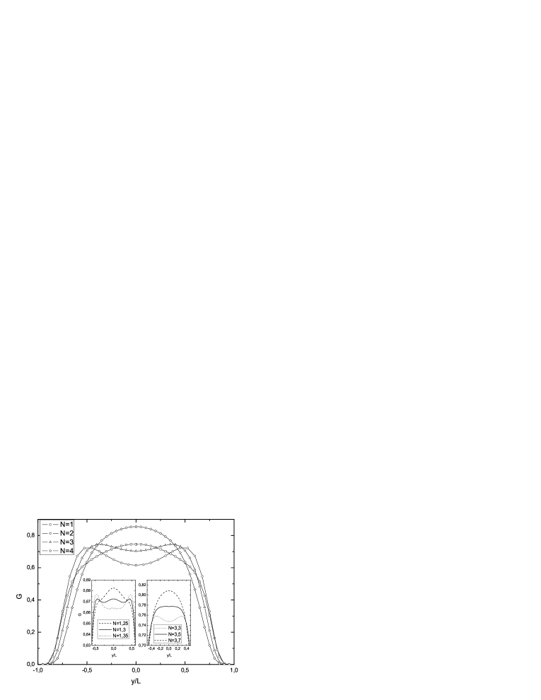
Figure 1: Normalized distribution function $G(\mathbf{t_{0}},x=0,y,N)$ for various chain lengths, computed with $20\times 20$ matrices. The insets show the distribution function at the onset of bimodality, and in the region of its disappearance.

using the truncations with $20\times 20$ order matrices and restricting the summation over the quantum number $l$ at $l=8$, are given in Fig. 1. The results show that the distribution function possesses the bimodal shape at intermediate chain lengths within the interval $N\in 1.3,...,3.5$. We also find that the distribution function becomes Gaussian for very short and very long chains. At the onset there is a tiny maximum at $y=0$, which we interpret as remnant of the Gaussian behavior of short chains. The maximum at $y=0$ for 3d chain is a rather small effect, which is difficult to be explained in a qualitative way.

We now will discuss qualitatively the origin of the bimodal behavior of the projected distribution function of the free end of the wormlike chain. The very short wormlike chain behaves similar to a weakly bending stiff rod, so that the distribution function of the free end is Gaussian with the maximum at $y=0$. The typical conformation of the chain in this regime looks like a bending rod with constant sign of curvature along the chain. For larger contour lengths the curvature fluctuations are small and are still controlled by the bending energy, however with varying sign of curvatures along the chain. The typical conformation of the chain can be imagined as undulations along the average conformation of the polymer. The projected distribution function of the free end in this regime is expected to be roughly uniform within some range of $y$. We expect that the inhomogeneities of curvature fluctuations in the vicinity of the clamped end are the reason for the maximum at $y\neq 0$. The larger curvatures in the vicinity of the fixed end result in larger displacements $y$ of the free end, and therefore contribute preferentially to the maximum at $y\neq 0$. With further increase of $N$ the conformations correspond to undulations around the average conformation of the chain, which is now a meandering line. Fluctuations become now less controlled by bending energy, which results in weakening of the bimodality. Since the difference between 2d and 3d chain is assumed to be marginal for short chains on the projected distribution function, we will compare the onset of the bimodality in both cases. Because the transversal displacement is measured in both cases in units of the contour length, we have to recompute the number of segments for 3d and 2d chain at the onset according to

$$N(3)=\frac{L}{L_{p}(3)}=\frac{L_{p}(2)}{L_{p}(3)}\frac{L}{L_{p}(2)}=\frac{L_{p}(2)}{L_{p}(3)}N(2).$$

Using the dependence of the persistence length on dimensionality benetatos05 , $L_{p}(3)\sim 1/(d-1)$, we obtain $N(3)=2N(2)$. According to lattanzi04 $N(2)\approx 0.75$ at the onset, hence we obtain $N(3)\approx 1.5$, which is not far from our numerical result, $N(3)\approx 1.3$ (see Fig. 1).

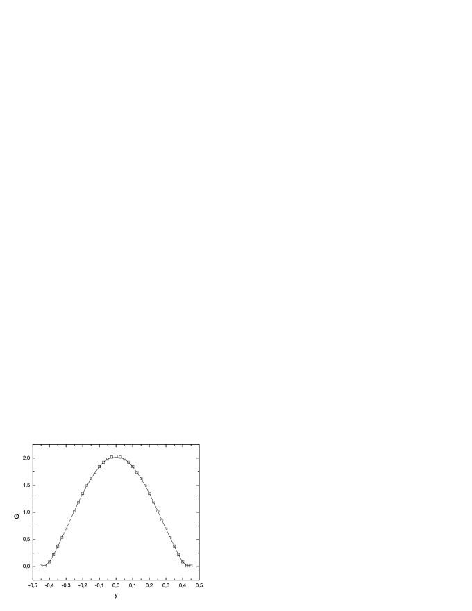
Figure 2: Normalized distribution function $G(\mathbf{t_{0}},x=0,y,N)$ for chain length $N=0.5$. Squares: truncation with $13\times 13$ matrices; continuous line: truncation with $20\times 20$ matrices.

We now will address the issues of accuracy of the calculations, which depends on the size of the matrices $D$ and $M^{s}$, and the maximal $l$ at which the summation over $l$ is stopped. In order to check our computation we verified that at large $N$ ($N=100$) the numerical evaluation of (4) gives with very high accuracy the Gaussian distribution $3/(2N)\,\exp(-3y^{2}/4N)$. The general tendency is such that the sufficient level of matrix truncations and the number of terms in the expansion over the Legendre polynomials increase with decreasing $N$. In the limit $N\rightarrow 0$ the whole series over $l$ should be taken into account. The accuracy of the computations is demonstrated in Fig. 2 showing the computation of the distribution function for $N=0.5$. The squares and the continuous curve correspond to the truncations by $13\times 13$ matrices and $20\times 20$ matrices, respectively. In both cases the summation was stopped at $l=8$. The corrections due to higher $l$-s are negligibly small. For example, the corrections associated with $l=10$ and $l=12$ contribute only in 3rd and 5th decimal digits, respectively. Thus, the computations depicted in Figs. 1, 2 can be considered as exact.

Figure 3 shows the results of the computation of the 3d distribution functions $G_{0}(r,N)$ of the free polymer obtained by performing the inverse Laplace-Fourier transform of the term $l=0$ in Eq. (1) for different chain lengths, and its comparison with the Monte Carlo simulations wilhelm96 .

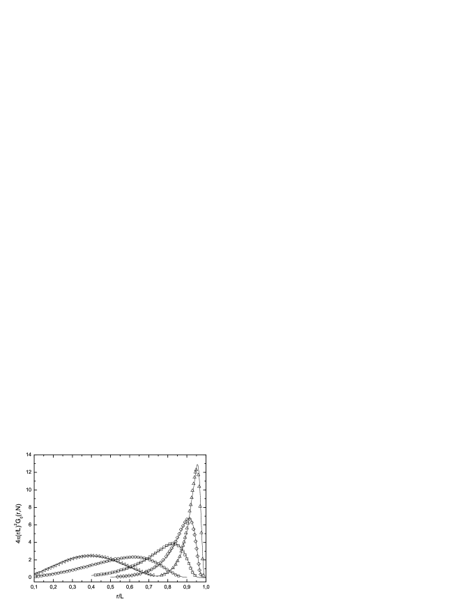
Figure 3: The end-to-end distribution function of a free polymer. Solid lines: the distribution function of a free three dimensional polymer chain for $N=10$, $5$, $2$, $1$, $0.5$ (from left to right) computed with $20\times 20$ matrices. The symbols are the Monte Carlo simulation data extracted from Fig. 1 in wilhelm96 .

Our results are in excellent agreement with the numerical data.

IV Conclusion

To conclude, we have studied the transverse distribution function of the free end of the three dimensional wormlike chain with fixed orientation and position of the second end using the exact solution for the Green’s function of the wormlike chain. Within the procedure of truncations of the exact formula with finite order matrices we find that the distribution function $G(\mathbf{t}_{0},x=0,y,N)$ for intermediate chain lengths, belonging to the interval $1.3L_{p},...,3.5L_{p}$, possesses the bimodal shape with the maxima at a finite value of the transverse displacement, which is consistent with the recent studies lattanzi04 ; benetatos05 and spakowitz05 for the two dimensional chain. In contrast to the 2d wormlike chain, the transverse 1d distribution function of the 3d chain shows only a tiny peak at $y=0$ in the vicinity of the onset of bimodality, which however disappears for larger $N$. We present also results of analytical considerations for short and large polymers which are in complete agreement with the classical works daniels52 ; gobush72 ; yamakawa73 where these limits were investigated using different methods. The computation of the three dimensional distribution function of a free polymer is in excellent agreement with the Monte Carlo simulations wilhelm96 .

- (1) S. F. Edwards, Proc. Phys. Soc. 85, 613 (1965).
- (2) P. G. de Gennes, Rep. Prog. Phys. 32, 187 (1969).
- (3) P. G. de Gennes, Scaling Concepts in Polymer Physics (Cornell University Press, Ithaca, NY, 1979).
- (4) M. Doi and S. F. Edwards, The Theory of Polymer Dynamics (Clarendon, Oxford, 1986).
- (5) J. des Cloizeaux and G. Jannink, Polymers in Solution, Their Modeling, and Structure (Oxford University Press, Oxford, 1990).
- (6) L. Schäfer, Excluded Volume Effects in Polymer Solutions (Springer, Berlin, 1999).
- (7) O. Kratky and G. Porod, Recl. Trav. Chim. Pays-Bas 68, 1106 (1949).
- (8) J. J. Hermans and R. Ullman, Physica 18, 951 (1952).
- (9) H. S. Daniels, Proc. R. Soc. Edin. A 63, 29 (1952).
- (10) S. Heine, O. Kratky and J. Roppert, Makromol. Chem. 56, 150 (1962).
- (11) N. Saito, K. Takahashi and Y. J. Yunoki, Phys. Soc. Japan 22, 219 (1967).
- (12) K. F. Freed, Adv. Chem. Phys. 22, 1 (1972).
- (13) M. Fixman and J. J. Kovac, J. Chem. Phys. 58, 1564 (1973).
- (14) J. des Cloizeaux, Macromolecules 6, 403 (1973).
- (15) T. Yoshizaki and H. Yamakawa, Macromolecules 13, 1518 (1980).
- (16) M. Warner, J. M. F. Gunn, and A. B. Baumgartner, J. Phys. A: Math. Gen. 18, 3007 (1985).
- (17) A. Kholodenko, Ann. Phys. 202, 186 (1990); J. Chem. Phys. 96, 700 (1991).
- (18) W. Gobush, H. Yamakawa, W. H. Stockmayer, and W. S. Magee, J. Chem. Phys. 57, 2839 (1972).
- (19) H. Yamakawa and M. Fujii, J. Chem. Phys. 59, 6641 (1973).
- (20) H. Yamakawa, Helical Wormlike Chains in Polymer Solutions (Springer, Berlin, 1997).
- (21) J. Wilhelm and E. Frey, Phys. Rev. Lett. 77, 2581 (1996).
- (22) G. Gompper and T. W. Burkhardt, Phys. Rev. A 40, R6124 (1989); Macromolecules 31, 2679 (1998).
- (23) E. Frey, K. Kroy, J. Wilhelm, and E. Sackmann, Dynamical Networks in Physics and Biology ed G Forgacs and D Beysens (Springer, Berlin, 1998).
- (24) G. S. Chirikjian and Y. F. Wang, Phys. Rev. E 62, 880 (2000).
- (25) J. Samuel and S. Sinha Phys. Rev. E 66, 050801(R) (2002).
- (26) A. Dhar and D. Chaudhuri, Phys. Rev. Lett. 89, 065502 (2002).
- (27) S. Stepanow and G. M. Schütz, Europhys. Lett. 60, 546 (2002).
- (28) R. G. Winkler, J. Chem. Phys. 118, 2919 (2003).
- (29) A. J. Spakowitz and Z.-G. Wang, Macromolecules 37, 5814 (2004).
- (30) G. A. Carri and M. Marucho, J. Chem. Phys. 121, 6064 (2004).
- (31) B. Hamprecht, W. Janke, and H. Kleinert, Phys. Lett. A 330, 254 (2004).
- (32) J. F. Marko and E. D. Siggia, Macromolecules 28, 8759 (1995).
- (33) S. Stepanow, Eur. Phys. J. B 39, 499 (2004).
- (34) S. Stepanow, J. Phys.: Condens. Matter 17, 1799 (2005).
- (35) J.-F. Allemand, S. Coccoa, N. Douarche, and G. Lia, Eur. Phys. J. E 19, 293 (2006).
- (36) T. Shimada, M. Doi, and K. Okano, J. Chem. Phys. 88, 2815 (1988).
- (37) G. Lattanzi, T. Munk, and E. Frey, Phys. Rev. E 69, 021801 (2004).
- (38) P. Benetatos, T. Munk, and E. Frey, Phys. Rev. E 72, 030801 (R) (2005).
- (39) A. J. Spakowitz and Z.-G. Wang, Phys. Rev. E 72, 041802 (2005).
- (40) Handbook of Mathematical Functions, ed. M. Abramowitz and I. A. Stegun (Dover Publications, New York, 1965).
- (41) L. D. Landau and E. M. Lifshitz, Quantum Mechanics (Nauka, Moscow, 1984), §34.