Variational study of hard-core bosons in a 2–D optical lattice using Projected Entangled Pair States (PEPS)

Abstract

We have studied the system of hard–core bosons on a 2–D optical lattice using a variational algorithm based on projected entangled-pair states (PEPS). We have investigated the ground state properties of the system as well as the responses of the system to sudden changes in the parameters. We have compared our results to mean field results based on a Gutzwiller ansatz.

I Introduction

Systems of interacting bosons in optical lattices have attracted a lot of interest in the last few years due to recent experimental achievements Greiner et al. (2002); Stöferle et al. (2004); Paredes et al. (2004); Tolra et al. (2004); Greiner et al. (2001); Moritz et al. (2003). In these systems, atoms are trapped by the combination of a periodic and a harmonic potential created by counterpropagating laser–beams. These systems of trapped atoms resemble a crystal in the sense that atoms are localized at periodic locations. The theoretical study of the static and dynamic properties of these systems is quite challenging. An exact solution can only be obtained in one dimension in the so–called Tonks–Girardeau limit via fermionization Girardeau (1960); Paredes et al. (2004). Outside this limit and in higher dimensions, approximate methods have to be used. The most common of those, the mean field approximation based on a Gutzwiller ansatz Jaksch et al. (2002), is unfortunately known to give imprecise predictions for correlations. The most powerful numerical methods such as the Density Matrix Renormalization Group (DMRG) White (1992) and Quantum Monte Carlo (QMC) are also of limited use: DMRG is mainly restricted to 1–D systems and QMC suffers from the sign–problem as time–evolutions are investigated.

In this paper, we apply the algorithm introduced in Verstraete and Cirac (2004). This algorithm is a variational method within a class of states termed Projected Entangled–Pair States (PEPS). It has been proven to work well for the Heisenberg antiferromagnet Verstraete and Cirac (2004) and the frustrated Shastry-Sutherland model Isacsson and Syljuasen (2006). The system we focus on is the system of hard–core bosons in a 2–D optical lattice. This model captures the essential physics of bosons in optical lattices Aizenman et al. (2004). We use the algorithm to determine the ground state properties of the system and to study the responses of the system to sudden changes in the parameters. We compare our results to mean field results based on the Gutzwiller ansatz. We find that the PEPS and the Gutzwiller ansatz deviate clearly in the prediction of the ground state momentum distribution and the time–evolution of the condensed fraction of the particles.

The paper is outlined as follows: In section II we give a brief overview of the algorithm. We specify the model we want to investigate in section III and explain the way the algorithm is applied to this model in section IV. The results of the numerical calculations are presented in sections V and VI. We conclude with the discussion of the the performance and the stability of the algorithm in section VII.

II The Algorithm

Although the algorithm has already been outlined in Verstraete and Cirac (2004), we reiterate it here in detail - specialized for our purpose. The algorithm is a variational method with respect to the class of PEPS. These states have been found to be adequate for representing the ground state of numerous many–body systems. Also, these states are favorable to variational calculations because they possess an internal refinement parameter, the virtual dimension $D$, that allows to control the precision of the calculation. While $D=1$ specializes the PEPS to a product state, the choice $D=d^{M}$ (with $M$ being the total number of lattice sites and $d$ the dimension of one subsystem) enlarges the space of PEPS to the complete Hilbert–space of the system. The purpose of the algorithm is - in our case - to simulate the time–evolution of a system within the subset of PEPS with a fixed $D$. This means that after each time–evolution step the state of the system is approximated by the ”nearest” PEPS with virtual dimension $D$. The key element of the algorithm is thus the optimization of the parameters of a PEPS such that its distance to a given state is minimized.

The manner in which the optimization is performed is closely related to the structure of PEPS. A PEPS is a state with coefficients that are contractions of tensors according to a certain scheme. Thereby, each tensor is associated with a physical subsystem. The contraction–scheme mimics the underlying lattice structure. Each tensor possesses one physical index with dimension equal to the physical dimension $d$ of a subsystem and a certain number of virtual indices with dimension $D$. The number of virtual indices is equal to the number of bonds that emanate from the lattice–site the tensor is associated with. For example, in a rectangular lattice the number of virtual indices is $4$ (except at the borders) - related to the left, right, upper and lower bond respectively. The tensor associated with site $i$ is

$$\big{[}A_{i}\big{]}^{k}_{lrud}$$

with physical index $k$ and virtual indices $l$, $r$, $u$ and $d$. The coefficients of the PEPS are then formed by joining the tensors in such a way that all indices related to same bonds are contracted. This is illustrated in fig. 1 for the special case of a $4\times 4$ square lattice. Assuming this contraction of tensors is performed by the function $\mathcal{F}(\cdot)$, the resulting PEPS can be written as

$$|\,\Psi_{A}\,\rangle=\sum_{k_{1},...,k_{M}=1}^{d}\mathcal{F}\big{(}\big{[}A_{1}\big{]}^{k_{1}},...,\big{[}A_{M}\big{]}^{k_{M}}\big{)}|\,k_{1},...,k_{M}\,\rangle.$$

Figure 1: Structure of the coefficient related to the state $|\,k_{11},..,k_{44}\,\rangle$ in the PEPS $|\,\Psi_{A}\,\rangle$. The bonds represent the indices of the tensors $[A_{i}]^{k}$ that are contracted.

The aim of the algorithm is to optimize the tensors $A_{i}$ such that the distance between the PEPS $|\,\Psi_{A}\,\rangle$ and a given state tends to a minimum. We assume that the given state is a PEPS $|\,\Psi_{B}\,\rangle$ with virtual dimension $D_{B}$ and tensors $B_{i}$. This is no loss of generality since every state can be written as a PEPS. The function to be minimized is then

$$K\big{(}A_{1},...,A_{M}\big{)}=\big{\|}|\,\Psi_{A}\,\rangle-|\,\Psi_{B}\,\rangle\big{\|}^{2}.$$

This function is non–convex with respect to all parameters $\{A_{1},...,A_{M}\}$. However, due to the special structure of PEPS, it is quadratic in the parameters $A_{i}$ associated with one lattice–site $i$. Because of this, the optimal parameters $A_{i}$ can simply be found by solving a system of linear equations. The concept of the algorithm is to do this one–site optimization site-by-site until convergence is reached.

The challenge that remains is to calculate the coefficient matrix and the inhomogenity of the linear equations–system. In principle, this is done by contracting all indices in the expressions for the scalar–products $\langle\,\Psi_{A}\,|\,\Psi_{A}\,\rangle$ and $\langle\,\Psi_{A}\,|\,\Psi_{B}\,\rangle$ except those connecting to  $A_{i}$. By interpreting the tensor $A_{i}$ as a $dD^{4}$-dimensional vector $\boldsymbol{A}_{i}$, these scalar–products can be written as

$$\langle\,\Psi_{A}\,|\,\Psi_{A}\,\rangle = \boldsymbol{A}_{i}^{\dagger}\mathcal{N}_{i}\boldsymbol{A}_{i}$$ (1)

$$\langle\,\Psi_{A}\,|\,\Psi_{B}\,\rangle = \boldsymbol{A}_{i}^{\dagger}\mathcal{W}_{i}.$$ (2)

Since

$$K=\langle\,\Psi_{B}\,|\,\Psi_{B}\,\rangle+\langle\,\Psi_{A}\,|\,\Psi_{A}\,\rangle-2Re\langle\,\Psi_{A}\,|\,\Psi_{B}\,\rangle,$$

the minimum is attained as

$$\mathcal{N}_{i}\boldsymbol{A}_{i}=\mathcal{W}_{i}.$$

The obstacle, however, is that the numerical calculation of the coefficient matrix $\mathcal{N}_{i}$ and the inhomogenity $\mathcal{W}_{i}$ requires a number of operations that scales exponentially with the number of subsystems $M$. This will make the algorithm non–efficient as the system grows larger. Because of this, an approximate method has to be used to calculate $\mathcal{N}_{i}$ and $\mathcal{W}_{i}$.

Figure 2: Structure of the contractions in $\langle\,\Psi_{A}\,|\,\Psi_{A}\,\rangle$. In this scheme, the first and last rows can be interpreted as MPS $|\,U_{1}\,\rangle$ and $\langle\,U_{4}\,|$ and the rows in between as MPO $U_{2}$ and $U_{3}$. The contraction of all tensors is then equal to $\langle\,U_{4}\,|U_{3}U_{2}|\,U_{1}\,\rangle$.

The approximate method suggested in Verstraete and Cirac (2004) is based on matrix product states (MPS) and matrix product operators (MPO). To see how MPS and MPO implicitly appear in the problem of calculating $\mathcal{N}_{i}$ and $\mathcal{W}_{i}$, we take a closer look at the structure of the contractions in the scalar–products $\langle\,\Psi_{A}\,|\,\Psi_{A}\,\rangle$ and $\langle\,\Psi_{A}\,|\,\Psi_{B}\,\rangle$. Thereby, we focus on a $L\times L$ square lattice in the following. We start with the study of $\langle\,\Psi_{A}\,|\,\Psi_{A}\,\rangle$. For this, we single out a specific site $j$ and define the $D^{2}\times D^{2}\times D^{2}\times D^{2}$–tensor

$$\big{[}E_{j}\big{]}_{(ll^{\prime})(rr^{\prime})}^{(uu^{\prime})(dd^{\prime})}=\sum_{k=1}^{d}\big{[}A_{j}^{*}\big{]}_{lrud}^{k}\big{[}A_{j}\big{]}_{l^{\prime}r^{\prime}u^{\prime}d^{\prime}}^{k}.$$

In this definition, the symbols $(ll^{\prime})$, $(rr^{\prime})$, $(uu^{\prime})$ and $(dd^{\prime})$ indicate composite indices. We may interpret the $4$ indices of this tensor as being related to the $4$ bonds emanating from site $j$ in the lattice. Then, $\langle\,\Psi_{A}\,|\,\Psi_{A}\,\rangle$ is formed by joining all tensors $E_{j}$ in such a way that all indices related to same bonds are contracted – as in the case of the coefficients of PEPS. These contractions have a rectangular structure, as depicted in fig. 2. In terms of the function $\mathcal{F}(\cdot)$, the scalar–product reads

$$\langle\,\Psi_{A}\,|\,\Psi_{A}\,\rangle=\mathcal{F}\big{(}E_{1},...,E_{M}\big{)}.$$

The main idea of the approximate algorithm is to interpret the first and the last row in this contraction–structure as MPS and the rows in between as MPO. The horizontal indices thereby form the virtual indices and the vertical indices are the physical indices. Thus, the MPS and MPO have both virtual dimension and physical dimension equal to $D^{2}$. Explicitly written, the MPS read

$$|\,U_{1}\,\rangle = \sum_{\tilde{d}_{1},...,\tilde{d}_{L}=1}^{D^{2}}\textrm{tr}\Big{(}\big{[}E_{11}\big{]}^{1\tilde{d}_{1}}\cdots\big{[}E_{1L}\big{]}^{1\tilde{d}_{L}}\Big{)}|\,\tilde{d}_{1},...,\tilde{d}_{L}\,\rangle$$

$$\langle\,U_{L}\,| = \sum_{\tilde{u}_{1},...,\tilde{u}_{L}=1}^{D^{2}}\textrm{tr}\Big{(}\big{[}E_{L1}\big{]}^{\tilde{u}_{1}1}\cdots\big{[}E_{LL}\big{]}^{\tilde{u}_{L}1}\Big{)}\langle\,\tilde{u}_{1},...,\tilde{u}_{L}\,|$$

and the MPO at row $r$ is

$$\begin{split}U_{r}=\sum_{\begin{subarray}{1}\tilde{u}_{1},...,\tilde{u}_{L}=1\\ \tilde{d}_{1},...,\tilde{d}_{L}=1\end{subarray}}^{D^{2}}&\textrm{tr}\Big{(}\big{[}E_{r1}\big{]}^{\tilde{u}_{1}\tilde{d}_{1}}\cdots\big{[}E_{rL}\big{]}^{\tilde{u}_{L}\tilde{d}_{L}}\Big{)}\times\\ &\times|\,\tilde{u}_{1},...,\tilde{u}_{L}\,\rangle\langle\,\tilde{d}_{1},...,\tilde{d}_{L}\,|.\end{split}$$

In terms of these MPS and MPO, the scalar–product is a product of MPO and MPS:

$$\langle\,\Psi_{A}\,|\,\Psi_{A}\,\rangle=\langle\,U_{L}\,|U_{L-1}\cdots U_{2}|\,U_{1}\,\rangle$$

The evaluation of this expression is, of course, intractable. With each multiplication of a MPO with a MPS, the virtual dimension increases by a factor of $D^{2}$. Thus, after $L$ multiplications, the virtual dimension is $D^{2L}$ – which is exponential in the number of rows. The expression, however, reminds of the time–evolution of a MPS Verstraete et al. (2004); Daley et al. (2004); Vidal (2004). There, each multiplication with a MPO corresponds to one evolution–step. The problem of the exponential increase of the virtual dimension is circumvented by restricting the evolution to the subspace of MPS with a certain virtual dimension $\tilde{D}$. This means that after each evolution–step the resulting MPS is approximated by the ”nearest” MPS with virtual dimension $\tilde{D}$. This approximation can be done efficiently, as shown in Verstraete et al. (2004). In this way, also $\langle\,\Psi_{A}\,|\,\Psi_{A}\,\rangle$ can be calculated efficiently: first, the MPS $|\,U_{2}\,\rangle$ is formed by multiplying the MPS $|\,U_{1}\,\rangle$ with MPO $U_{2}$. The MPS $|\,U_{2}\,\rangle$ is then approximated by $|\,\tilde{U}_{2}\,\rangle$ with virtual dimension $\tilde{D}$. In this fashion the procedure is continued until $|\,\tilde{U}_{L-1}\,\rangle$ is obtained. The scalar–product $\langle\,\Psi_{A}\,|\,\Psi_{A}\,\rangle$ is then simply

$$\langle\,\Psi_{A}\,|\,\Psi_{A}\,\rangle=\langle\,U_{L}\,|\,\tilde{U}_{L-1}\,\rangle.$$

The calculation of the coefficient matrix $\mathcal{N}_{i}$ is closely related to the calculation of $\langle\,\Psi_{A}\,|\,\Psi_{A}\,\rangle$: $\mathcal{N}_{i}$ relies on the contraction of all but one of the tensors $E_{j}$ according to the same scheme as before. The one tensor that has to be omitted is $E_{i}$ – the tensor related to site $i$. Assuming this contraction is performed by the function $\mathcal{G}_{i}(\cdot)$, $\mathcal{N}_{i}$ can be written as

$$\big{[}\mathcal{N}_{i}\big{]}_{lrud}^{k}{\phantom{\big{]}}}_{k^{\prime}}^{l^{\prime}r^{\prime}u^{\prime}d^{\prime}}=\mathcal{G}_{i}\big{(}E_{1},...,E_{M}\big{)}_{lrud}^{l^{\prime}r^{\prime}u^{\prime}d^{\prime}}\delta_{k^{\prime}}^{k}.$$

If we join the indices $(klrud)$ and $(k^{\prime}l^{\prime}r^{\prime}u^{\prime}d^{\prime})$, we obtain the $dD^{4}\times dD^{4}$–matrix that fulfills equation (1). To evaluate $\mathcal{G}_{i}(\cdot)$ efficiently, we proceed in the same way as before by interpreting the rows in the contraction–structure as MPS and MPO. First, we join all rows that lie above site $i$ by multiplying the topmost MPS $|\,U_{1}\,\rangle$ with subjacent MPO and reducing the dimension after each multiplication to $\tilde{D}$. Then, we join all rows lying below $i$ by multiplying $\langle\,U_{L}\,|$ with adjacent MPO and reducing the dimension as well. We end up with two MPS of virtual dimension $\tilde{D}$ – which we can contract efficiently with all but one of the tensors $E_{j}$ lying in the row of site $i$.

The scalar–product $\langle\,\Psi_{A}\,|\,\Psi_{B}\,\rangle$ and the inhomogenity $\mathcal{W}_{i}$ are calculated in an efficient way following the same ideas. First, the $DD_{B}\times DD_{B}\times DD_{B}\times DD_{B}$–tensors

$$\big{[}F_{j}\big{]}_{(ll^{\prime})(rr^{\prime})}^{(uu^{\prime})(dd^{\prime})}=\sum_{k=1}^{d}\big{[}A_{j}^{*}\big{]}_{lrud}^{k}\big{[}B_{j}\big{]}_{l^{\prime}r^{\prime}u^{\prime}d^{\prime}}^{k}.$$

are defined. The scalar–product $\langle\,\Psi_{A}\,|\,\Psi_{B}\,\rangle$ is then obtained by contracting all tensors $F_{j}$ according to the previous scheme – which is performed by the function $\mathcal{F}(\cdot)$:

$$\langle\,\Psi_{A}\,|\,\Psi_{B}\,\rangle=\mathcal{F}\big{(}F_{1},...,F_{M}\big{)}$$

The inhomogenity $\mathcal{W}_{i}$ relies on the contraction of all but one of the tensors $F_{j}$, namely the function $\mathcal{G}_{i}\big{(}\cdot)$, in the sense that

$$\big{[}\mathcal{W}_{i}\big{]}_{lrud}^{k}=\sum_{l^{\prime}r^{\prime}u^{\prime}d^{\prime}=1}^{D}\mathcal{G}_{i}\big{(}F_{1},...,F_{M}\big{)}_{lrud}^{l^{\prime}r^{\prime}u^{\prime}d^{\prime}}\big{[}B_{i}\big{]}_{l^{\prime}r^{\prime}u^{\prime}d^{\prime}}^{k}.$$

Joining all indices $(klrud)$ in the resulting tensor leads to the vector of length $dD^{4}$ that fulfills equation (2). Thus, both the scalar–product $\langle\,\Psi_{A}\,|\,\Psi_{B}\,\rangle$ and the inhomogenity $\mathcal{W}_{i}$ are directly related to the expressions $\mathcal{F}\big{(}F_{1},...,F_{M}\big{)}$ and $\mathcal{G}_{i}\big{(}F_{1},...,F_{M}\big{)}$. These expressions, however, can be evaluated efficiently using the approximate method from before.

Summing up, we have an algorithm that allows the efficient reduction of the virtual dimension of a PEPS - and thus the efficient simulation of a time–evolution step within the subset of PEPS.

III The Model: hard–core bosons in a 2–D optical lattice

This algorithm we use to study a system of bosons in a 2–D optical lattice of size $L\times L$. This system is characterized by the Bose–Hubbard Hamiltonian

$$H=-J\sum_{<i,j>}\big{(}a_{i}^{\dagger}a_{j}+h.c.\big{)}+\frac{U}{2}\sum_{i}\hat{n}_{i}(\hat{n}_{i}-1)+\sum_{i}V_{i}\hat{n}_{i},$$

where $a^{\dagger}_{i}$ and $a_{i}$ are the creation and annihilation operators on site $i$ and $\hat{n}_{i}=a^{\dagger}_{i}a_{i}$ is the number operator. This Hamiltonian describes the interplay between the kinetic energy due to the next-neighbor hopping with amplitude $J$ and the repulsive on-site interaction $U$ of the particles. The last term in the Hamiltonian models the harmonic confinement of magnitude $V_{i}=V_{0}(i-i_{0})^{2}$. Since the total number of particles $\hat{N}=\sum_{i}\hat{n}_{i}$ is a symmetry of the Hamiltonian, the ground–state will have a fixed number of particles $N$. We choose this number by appending the term $-\mu\hat{N}$ to the Hamiltonian and tuning the chemical potential $\mu$. The variation of the ratio $U/J$ drives a phase-transition between the Mott-insulating and the superfluid phase, characterized by localized and delocalized particles respectively Fisher et al. (1989). Experimentally, the variation of $U/J$ can be realized by tuning the depth of the optical lattice Jaksch et al. (1998); Büchler et al. (2003). The quantity that is typically measured is the momentum distribution. The is done by letting the atomic gas expand and measuring the density distribution of the expanded cloud. Thus, we will be mainly interested here in the (quasi)–momentum distribution

$$n_{k}=\frac{1}{L^{2}}\sum_{r,s}\langle a^{\dagger}_{r}a_{s}\rangle e^{i2\pi k\cdot(r-s)/L^{2}}$$

of the particles.

In the following, we focus on the limit of a hard–core interaction, $U/J\to\infty$. In this limit, two particles are prevented from occupying a single site. This limit is especially interesting in one dimension where the particles form the so–called Tonks-Girardeau gas Girardeau (1960); Paredes et al. (2004). The particles in this gas are strongly correlated – which leads to algebraically decaying correlation functions. In two dimensions, the model was studied in detail in Aizenman et al. (2004). In the hard–core limit, the Bose–Hubbard model is equivalent to a spin–system with $XX$–interactions described by the Hamiltonian

$$H=-\frac{J}{2}\sum_{<i,j>}\big{(}\sigma_{x}^{(i)}\sigma_{x}^{(j)}+\sigma_{y}^{(i)}\sigma_{y}^{(j)}\big{)}+\frac{1}{2}\sum_{i}\big{(}V_{i}-\mu\big{)}\sigma_{z}^{(i)}.$$

Here, $\sigma_{x}^{(i)}$, $\sigma_{y}^{(i)}$ and $\sigma_{z}^{(i)}$ denote the Pauli-operators acting on site $i$. This Hamiltonian has the structure we can simulate with the algorithm: it describes $L^{2}$ physical systems of dimension $d=2$ on a $L\times L$–square lattice.

IV Application of the algorithm to hard–core bosons in a 2–D lattice

The principle of simulating a time–evolution step according to $XX$–Hamiltonian is as follows: first, a PEPS $|\,\Psi_{A}^{0}\,\rangle$ with physical dimension $d=2$ and virtual dimension $D$ is chosen as a starting state. This state is evolved by the time–evolution operator $U=e^{-iH\delta t}$ (we assume $\hbar=1$) to yield another PEPS $|\,\Psi_{B}\,\rangle$ with increased virtual dimension $D_{B}$:

$$|\,\Psi_{B}\,\rangle=U|\,\Psi_{A}^{0}\,\rangle$$

The virtual dimension of this state is then reduced to $D$ by applying the algorithm of the previous section. This means, a new PEPS $|\,\Psi_{A}\,\rangle$ with virtual dimension $D$ is calculated that has minimal distance to $|\,\Psi_{B}\,\rangle$. This new PEPS is then the starting state for the next time–evolution step.

The operator $U$, however, increases the virtual dimension of a PEPS by a factor that scales exponentially with $L$. This is why it is more convenient to approximate $U$ by an operator that increases the virtual dimension merely by a constant factor $\eta$. This is done by means of a Trotter–approximation: first, the interaction–terms are classified in horizontal and vertical according to their orientation and in even and odd depending on whether the interaction is between even–odd or odd–even rows (or columns). The Hamiltonian can then be decomposed into a horizontal–even, a horizontal–odd, a vertical–even and a vertical–odd part:

$$H=H_{he}+H_{ho}+H_{ve}+H_{vo}$$

The single–particle operators of the Hamiltonian can simply be incorporated in one of the four parts. Using the Trotter–approximation, the time–evolution operator $U$ can be written as a product of four evolution–operators:

$$U=e^{-iH\delta t}\approx e^{-iH_{he}\delta t}e^{-iH_{ho}\delta t}e^{-iH_{ve}\delta t}e^{-iH_{vo}\delta t}$$ (3)

Since each of the four parts of the Hamiltonian consists of a sum of commuting terms, each evolution–operator equals a product of two–particle operators

$$w_{ij}=e^{i\frac{\delta tJ}{2}\big{(}\sigma_{x}^{(i)}\sigma_{x}^{(j)}+\sigma_{y}^{(i)}\sigma_{y}^{(j)}\big{)}}$$

acting on neighboring sites $i$ and $j$. These two–particle operators have a Schmidt–decomposition consisting of $4$ terms:

$$w_{ij}=\sum_{\rho=1}^{4}u_{i}^{\rho}\otimes v_{j}^{\rho}$$

One such two–particle operator $w_{ij}$ applied to the PEPS $|\,\Psi_{A}^{0}\,\rangle$ modifies the tensors $A_{i}^{0}$ and $A_{j}^{0}$ associated with sites $i$ and $j$ as follows: assuming the sites $i$ and $j$ are horizontal neighbors, $A_{i}^{0}$ has to be replaced by

$$\big{[}B_{i}\big{]}^{k}_{l(r\rho)ud}=\sum_{k^{\prime}=1}^{2}\big{[}u_{i}^{\rho}\big{]}^{k}_{k^{\prime}}\big{[}A_{i}^{0}\big{]}^{k^{\prime}}_{lrud}$$

and $A_{j}^{0}$ becomes

$$\big{[}B_{j}\big{]}^{k}_{(l\rho)rud}=\sum_{k^{\prime}=1}^{2}\big{[}v_{j}^{\rho}\big{]}^{k}_{k^{\prime}}\big{[}A_{j}^{0}\big{]}^{k^{\prime}}_{lrud}.$$

These new tensors have a joint index related to the bond between sites $i$ and $j$. This joint index is composed of the original index of dimension $D$ and the index $\rho$ of dimension $4$ that enumerates the terms in the Schmidt–decomposition. Thus, the effect of the two–particle operator $w_{ij}$ is to increase the virtual dimension of the bond between sites $i$ and $j$ by a factor of $4$. Consequently, $e^{-iH_{he}\delta t}$ and $e^{-iH_{ho}\delta t}$ increase the dimension of every second horizontal bond by a factor of $4$; $e^{-iH_{ve}\delta t}$ and $e^{-iH_{vo}\delta t}$ do the same for every second vertical bond. By applying all four evolution–operators consecutively, we have found an approximate form of the time–evolution operator $U$ that – when applied to a PEPS – yields another PEPS with a virtual dimension multiplied by a constant factor $\eta=4$.

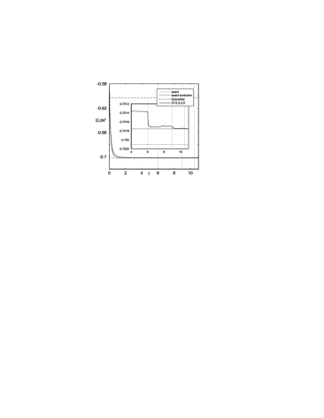
Figure 3: Energy as a function of time for the imaginary time–evolution of the system of hard–core bosons on a $4\times 4$–lattice. The evolutions are performed sequentially with PEPS of virtual dimension $D=2$, $D=3$, $D=4$ and $D=5$. The times at which $D$ is increased are indicated by vertical lines. For comparison, the exact ground state–energy, the exact imaginary time–evolution and the energy of the optimal Gutzwiller ansatz are included.

Even though the principle of simulating a time–evolution step has been recited now, the implementation in this form is numerically expensive. This is why we append some notes about how to make the simulation more efficient:
1.- Partitioning of the evolution: The number of required numerical operations decreases significantly as one time–evolution step is partitioned into $4$ substeps: first the state $|\,\Psi_{A}^{0}\,\rangle$ is evolved by $e^{-iH_{vo}\delta t}$ only and the dimension of the increased bonds is reduced back to $D$. Next, evolutions according to $e^{-iH_{ve}\delta t}$, $e^{-iH_{ho}\delta t}$ and $e^{-iH_{he}\delta t}$ follow. Even though the partitioning increases the number of evolution–steps by a factor of $4$, the number of multiplications in one evolution–step decreases by a factor of $\eta^{3}=64$.
2.- Optimization of the contraction order: Most critical for the efficiency of the numerical simulation is the order in which the contractions are performed. We have optimized the order in such a way that the scaling of the number of multiplications with the virtual dimension $D$ is minimal. For this, we assume that the dimension $\tilde{D}$ that tunes the accuracy of the approximate calculation of $\mathcal{N}_{i}$ and $\mathcal{W}_{i}$ is proportional to $D^{2}$, i.e. $\tilde{D}=\kappa D^{2}$. The number of required multiplications is then of order $\kappa^{2}D^{12}L^{2}$ and the required memory scales as $d\eta\kappa^{2}D^{8}$.
3.- Optimization of the starting state: The number of sweeps required to reach convergence depends on the choice of the starting state for the optimization. The idea for finding a good starting state is to reduce the bonds with increased virtual dimension $\eta D$ by means of a Schmidt–decomposition. This is done as follows: assuming the bond is between the horizontal neighboring sites $i$ and $j$, the contraction of the tensors associated with these sites, $B_{i}$ and $B_{j}$, along the bond $i$–$j$ forms the tensor

$$\big{[}\mathcal{M}_{ij}\big{]}^{k}_{lud}{\phantom{\big{]}}}^{k^{\prime}}_{r^{\prime}u^{\prime}d^{\prime}}=\sum_{\rho=1}^{D\eta}\big{[}B_{i}\big{]}^{k}_{l\rho ud}\big{[}B_{j}\big{]}^{k^{\prime}}_{\rho r^{\prime}u^{\prime}d^{\prime}}.$$

By joining the indices $(klud)$ and $(k^{\prime}r^{\prime}u^{\prime}d^{\prime})$, this tensor can be interpreted as a $dD^{3}\times dD^{3}$–matrix. The Schmidt–decomposition of this matrix is

$$\mathcal{M}_{ij}=\sum_{\rho=1}^{dD^{3}}c_{\rho}\mathcal{A}_{i}^{\rho}\otimes\mathcal{A}_{j}^{\rho}$$

with the Schmidt–coefficients $c_{\rho}$ ($c_{\rho}\geq 0$) and corresponding matrices $\mathcal{A}_{i}^{\rho}$ and $\mathcal{A}_{j}^{\rho}$. We can relate these matrices to a new pair of tensors $A_{i}^{0}$ and $A_{j}^{0}$ associated with sites $i$ and $j$:

$$\big{[}A_{i}^{0}\big{]}^{k}_{l\rho ud} = \sqrt{c_{\rho}}\big{[}\mathcal{A}_{i}^{\rho}\big{]}_{lud}^{k}$$

$$\big{[}A_{j}^{0}\big{]}^{k}_{\rho rud} = \sqrt{c_{\rho}}\big{[}\mathcal{A}_{j}^{\rho}\big{]}_{rud}^{k}$$

The virtual dimension of these new tensors related to the bond between sites $i$ and $j$ is equal to the number of terms in the Schmidt–decomposition. Since these terms are weighted with the Schmidt–coefficients $c_{\rho}$, it is justified to keep only the $D$ terms with coefficients of largest magnitude. Then, the contraction of the tensors $A_{i}^{0}$ and $A_{j}^{0}$ along the bond $i$–$j$ with dimension $D$ yields a good approximation to the true value $\mathcal{M}_{ij}$:

$$\big{[}\mathcal{M}_{ij}\big{]}^{k}_{lud}{\phantom{\big{]}}}^{k^{\prime}}_{r^{\prime}u^{\prime}d^{\prime}}\approx\sum_{\rho=1}^{D}\big{[}A_{i}^{0}\big{]}^{k}_{l\rho ud}\big{[}A_{j}^{0}\big{]}^{k^{\prime}}_{\rho r^{\prime}u^{\prime}d^{\prime}}.$$

This method applied to all bonds with increased dimension provides us with the starting state for the optimization.

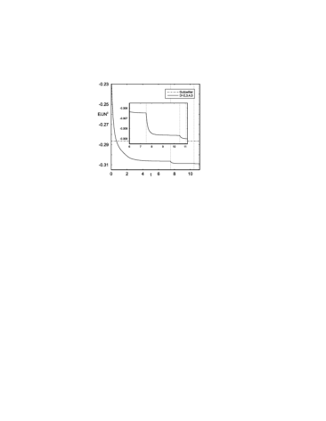
Figure 4: Energy as a function of time for the imaginary time–evolution of the system of hard–core bosons on a $11\times 11$–lattice. The evolutions are performed sequentially with PEPS of virtual dimension $D=2$, $D=3$, $D=4$ and $D=5$. The times at which $D$ is increased are indicated by vertical lines. For comparison, the energy of the optimal Gutzwiller ansatz is included.

V Ground state properties

In the following, we study the ground–state properties of the system of hard–core bosons for lattice–sizes $4\times 4$ and $11\times 11$. We calculate the ground–state by means of an imaginary time–evolution which we can simulate with the method from before.

We first focus on the $4\times 4$–lattice for which we can calculate the ground–state exactly and are able to estimate the precision of the algorithm by comparison with exact results. In fig. 3, the energy is plotted as the system undergoes the imaginary time–evolution. We thereby assume a time–step $\delta t=-i0.03$. We choose the magnitude of the harmonic confinement (in units of the tunneling–constant) $V_{0}/J=36$. In addition, we tune the chemical potential to $\mu/J=3.4$ such that the ground state has particle–number $N=4$. With this configuration, we perform the imaginary time–evolution both exactly and variationally with PEPS. As a starting state we take a product state that represents a Mott-like distribution with $4$ particles arranged in the center of the trap and none elsewhere. The variational calculation is performed with $D=2$ first until convergence is reached; then, evolutions with $D=3$, $D=4$ and $D=5$ follow. At the end, a state is obtained that is very close to the state obtained by exact evolution. The difference in energy is $|E_{D=5}-E_{exact}|\backsimeq 6.4614\cdot 10^{-5}J$. For comparison, also the exact ground–state energy obtained by an eigenvalue–calculation and the energy of the optimal Gutzwiller ansatz are included in fig. 3. The difference between the exact result and the results of the imaginary time–evolution is due to the Trotter–error and is of order $O(\delta t^{2})$. The energy of the optimal Gutzwiller-Ansatz is well seperated from the exact ground–state energy and the results of the imaginary time–evolution.

In fig. 4, the energy as a function of time is plotted for the imaginary time–evolution on the $11\times 11$–lattice. Again, a time–step $\delta t=-i0.03$ is assumed for the evolution. The other parameters are set as follows: the ratio between harmonic confinement and the tunneling constant is chosen as $V_{0}/J=100$ and the chemical potential is tuned to $\mu/J=3.8$ such that the total number of particles $N$ is $14$. The starting state for the imaginary time–evolution is, similar to before, a Mott-like distribution with $14$ particles arranged in the center of the trap. This state is evolved within the subset of PEPS with $D=2$, $D=3$, $D=4$ and $D=5$. As can be gathered from the plot, this evolution shows a definite convergence. In addition, the energy of the final PEPS lies well below the energy of the optimal Gutzwiller ansatz.

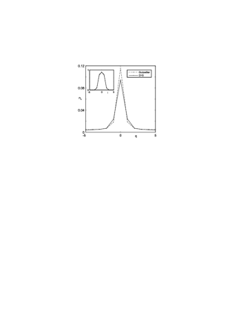
Figure 5: (Quasi)–momentum distribution of the particles in the ground state of a $11\times 11$–lattice. Plotted are results of the variational calculations with PEPS of dimension $D=5$ and with the Gutzwiller ansatz. From the inset, the density of the particles can be gathered.

The difference between the PEPS and the Gutzwiller ansatz becomes more evident as one studies the momentum distribution of the particles. The diagonal slice of the (quasi)–momentum distribution is shown in fig. 5. As can be seen, there is a clear difference between the momentum distribution derived from the PEPS and the one from the Gutzwiller ansatz. In contrast, the PEPS and the Gutzwiller ansatz produce a very similar density profile (see inset). The acceptability of the Gutzwiller ansatz is due to the inhomegenity of the system: the different average particle number at each site is the cause for the correlations between different sites. These correlations are, in many cases, good approximations. In contrast, the average particle number is constant in homogeneous systems – which leads to correlations that are constant. Thus, the Gutzwiller ansatz is expected to be less appropriate for the study of correlations of homogeneous systems.

VI Dynamics of the system

We now focus on the study of dynamic properties of hard–core bosons on a lattice of size $11\times 11$. We investigate the responses of this system to sudden changes in the parameters and compare our numerical results to the results obtained by the Gutzwiller ansatz. The property we are interested in is the fraction of particles that are condensed. For interacting and finite systems, this property is measured best by the condensate density $\rho$ which is defined as largest eigenvalue of the correlation–matrix $\langle a_{i}^{\dagger}a_{j}\rangle$.

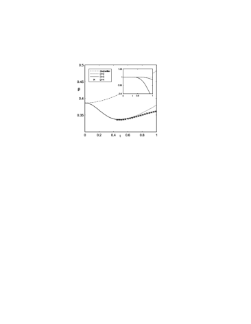
Figure 6: Time evolution of the condensate density after a sudden change of the magnitude of the trapping potential from $V_{0}/J=100$ to $V_{0}/J=64$. As a starting state, we use the Gutzwiller–approximation of the ground state. The evolution is performed on the basis of the Gutzwiller ansatz and PEPS with $D=2$, $D=3$ and $D=4$. From the inset, the overlap between the PEPS with $D=2$ and $D=3$ (solid line) and the PEPS with $D=3$ and $D=4$ (dashed line) can be gathered.

First, we study the time evolution of the condensate density after a sudden change of the trapping potential. We start with a Gutzwiller–approximation of the ground state in case of a trapping potential of magnitude $V_{0}/J=100$. The chemical potential we tune to $\mu/J=3.8$ to achieve an average particle–number of $\langle\hat{N}\rangle=14$. This state we expose to a trapping potential of magnitude $V_{0}/J=64$ and calculate the evolution of the condensate density using the Gutzwiller ansatz and PEPS with $D=2$, $D=3$ and $D=4$. We thereby assume a time–step $\delta t=0.03$. To assure that our results are accurate, we proceed as follows: first, we perform the simulation using PEPS with $D=2$ and $D=3$ until the overlap between these two states falls below a certain value. Then, we continue the simulation using PEPS with $D=3$ and $D=4$ as long as the overlap between these two states is close to $1$. The results of this calculation can be gathered from fig. 6. What can be observed is that the results obtained from using PEPS are qualitatively very different from the result based on the Gutzwiller ansatz. The inset in fig. 6 shows the overlap of the $D=2$ with the $D=3$–PEPS and the $D=3$ with the $D=4$–PEPS.

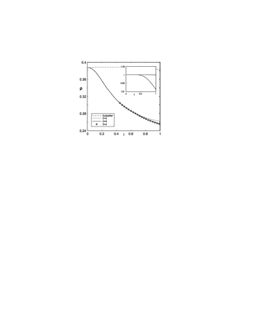
Figure 7: Time evolution of the condensate density after a sudden shift of the center of the trap by one site in $x$– and $y$–direction. Starting state is the Gutzwiller–approximation of the ground state. The evolution is performed using the Gutzwiller ansatz and PEPS with $D=2$, $D=3$ and $D=4$. The inset shows the overlap between the PEPS with $D=2$ and $D=3$ (solid line) and $D=3$ and $D=4$ (dashed line).

In fig. 7, the time–evolution of the condensate density after a sudden shift of the trapping potential is plotted. As a starting state, again the Gutzwiller–approximation of the ground state in a trap of magnitude $V_{0}/J=100$ is used. This state is evolved with respect to a trapping potential that is shifted by one lattice–site in $x$– and $y$–direction. We assume a time–step $\delta t=0.03$ and tune the chemical potential to $\mu/J=3.8$. As before, we perform the simulation successively with $D=2$, $D=3$ and $D=4$ and judge the accuracy of the results by monitoring the overlap between PEPS with different $D$s. From the plot, it can be gathered that the evolution of the condensate density based on the Gutzwiller ansatz is qualitatively again very different from the evolution obtained from using PEPS. The evolution obtained from using PEPS shows a definite damping. The shift of the trap thus provokes a destruction of the condensate. The evolution based on the Gutzwiller ansatz doesn’t show this feature.

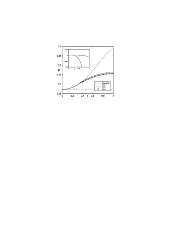
Figure 8: Time evolution of the condensate density starting from a Mott–distribution with $14$–particles arranged in the center of the trap. The magnitude of the trapping potential is $V_{0}/J=100$. For the evolution, the Gutzwiller ansatz and PEPS with $D=2$, $D=3$ and $D=4$ are used. The inset shows the overlap between the $D=2$ and $D=3$–PEPS (solid line) and the $D=3$ and $D=4$–PEPS (dashed line).

As a contrary example, we study the evolution of a Mott-distribution with $14$ particles arranged in the center of the trap. We assume $V_{0}/J=100$, $\mu/J=3.8$ and $\delta t=0.03$. We perform the simulation in the same way as before with $D=2$, $D=3$ and $D=4$. In fig. 8, the time evolution of the condensate density is plotted. It can be observed that there is a definite increase in the condensate fraction. The Gutzwiller ansatz is in contrast to this result since it predicts that the condensate density remains constant.

VII Accuracy and performance of the algorithm

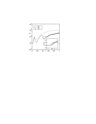
Figure 9: Distance $K$ between the time–evolved state and the state with reduced virtual dimension. The virtual dimensions $D=2$, $D=3$ and $D=4$ are included. The distance is plotted for the evolution of a Mott-distribution with $N=14$, as explained in fig. 8. From the inset, the deviation of the particle number from the value $14$ can be gathered.

Finally, we make a few comments about the accuracy and the performance of the algorithm. One indicator for the accuracy of the algorithm is the distance between the time–evolved state and the state with reduced virtual dimension. For the time–evolution of the Mott–distribution that was discussed in section VI, this quantity is plotted in fig. 9. We find that the distance is typically of order $10^{-3}$ for $D=2$ and of order $10^{-4}$ for $D=3$ and $D=4$. Another quantity we monitor is the total number of particles $\langle\hat{N}\rangle$. Since this quantity is supposed to be conserved during the whole evolution, its fluctiations indicate the reliability of the algorithm. From the inset in fig. 9, the fluctuations of the particle number in case of the time–evolution of the Mott–distribution can be gathered. We find that these fluctuations are at most of order $10^{-5}$.

The main bottleneck for the performance of the algorithm is the scaling of the number of required multiplications with the virtual dimension $D$. As mentioned in section IV, the number of required multiplications is of order $D^{12}$. Our simulations were run on a workstation with a $3.0$ GHz Intel Xeon processor. On such a system, one evolution step on a $11\times 11$–lattice with $D=5$ required a computing time of $55$ hours. Another bottleneck for the algorithm forms the scaling of the required memory with the virtual dimension $D$ – which is of order $D^{8}$. The simulation on a $11\times 11$–lattice with $D=5$ thereby required a main memory of $2$ GB. These bottlenecks make it difficult at the moment to go beyond a virtual dimension of $D=5$. Nonetheless, a virtual dimension of $D=5$ is expected to yield good results for many problems already. We intend to overcome the limitations of time and space by distributing tensor contractions among several processors in a future project.

VIII Conclusions

Summing up, we have studied the system of hard–core bosons on a 2–D lattice using a variational method based on PEPS. We have thereby investigated the ground state properties of the system and its responses to sudden changes in the parameters. We have compared our results to results based on the Gutzwiller ansatz. We have observed that the Gutzwiller ansatz predicts very well the density distribution of the particles. However, the momentum distribution obtained from the Gutzwiller ansatz is, though qualitatively similar, quantitatively clearly different from the distribution obtained from the PEPS ansatz. In addition, the PEPS and the Gutzwiller ansatz are very different in the prediction of time evolutions. We conclude that the Gutzwiller ansatz has to be applied carefully in these cases. The simulations done in this paper give a clear demonstration of the power of the PEPS-approach, both for finding ground states in higher-dimensional quantum spin systems and for simulating real-time evolution.

References

- Greiner et al. (2002) M. Greiner, O. Mandel, T. Esslinger, T. W. Hänsch, and I. Bloch, Nature 415, 39 (2002).
- Stöferle et al. (2004) T. Stöferle, H. Moritz, C. Schori, M. Köhl, and T. Esslinger, Phys. Rev. Lett. 92, 130403 (2004), eprint cond-mat/9312440.
- Paredes et al. (2004) B. Paredes, A. Widera, V. Murg, O. Mandel, S. Fölling, I. Cirac, G. V. Shlyapnikov, T. W. Hänsch, and I. Bloch, Nature 429, 277 (2004).
- Tolra et al. (2004) B. L. Tolra, K. M. O’Hara, J. H. Huckans, W. D. Phillips, S. L. Rolston, and J. V. Porto, Phys. Rev. Lett. 92, 190401 (2004), eprint cond-mat/0312003.
- Greiner et al. (2001) M. Greiner, I. Bloch, O. Mandel, T. W. Hänsch, and T. Esslinger, Phys. Rev. Lett. 87, 160405 (2001), eprint cond-mat/0105105.
- Moritz et al. (2003) H. Moritz, T. Stöferle, M. Köhl, and T. Esslinger, Phys. Rev. Lett. 91, 250402 (2003), eprint cond-mat/0307607.
- Girardeau (1960) M. Girardeau, J. Math. Phys. 1, 516 (1960).
- Jaksch et al. (2002) D. Jaksch, V. Venturi, J. I. Cirac, C. J. Williams, and P. Zoller, Phys. Rev. Lett. 89, 040402 (2002), eprint cond-mat/0204137.
- White (1992) S. R. White, Phys. Rev. Lett 69, 2863 (1992).
- Verstraete and Cirac (2004) F. Verstraete and J. I. Cirac (2004), eprint cond-mat/0407066.
- Isacsson and Syljuasen (2006) A. Isacsson and O. F. Syljuasen, Phys. Rev. E 74, 026701 (2006), eprint cond-mat/0604134.
- Aizenman et al. (2004) M. Aizenman, E. H. Lieb, R. Seiringer, J. P. Solovej, and J. Yngvason, Phys. Rev. A 70, 023612 (2004), eprint cond-mat/0412034.
- Verstraete et al. (2004) F. Verstraete, J. J. García-Ripoll, and J. I. Cirac, Phys. Rev. Lett 93, 207204 (2004), eprint cond-mat/0406426.
- Daley et al. (2004) A. J. Daley, C. Kollath, U. Schollwoeck, and G. Vidal, J. Stat. Mech.: Theor. Exp., P04005 (2004), eprint cond-mat/0403313.
- Vidal (2004) G. Vidal, Phys. Rev. Lett 93, 040502 (2004), eprint quant-ph/0310089.
- Fisher et al. (1989) M. P. Fisher, P. B. Weichmann, G. Grinstein, and D. S. Fisher, Phys. Rev. B 40, 546 (1989).
- Jaksch et al. (1998) D. Jaksch, C. Bruder, J. I. Cirac, C. W. Gardiner, and P. Zoller, Phys. Rev. Lett 81, 3108 (1998), eprint cond-mat/9805329.
- Büchler et al. (2003) H. P. Büchler, G. Blatter, and W. Zwerger, Phys. Rev. Lett. 90, 130401 (2003).