Time modulation of atom sources

Abstract

Sudden turn-on of a matter-wave source leads to characteristic oscillations of the density profile which are the hallmark feature of diffraction in time. The apodization of matter waves relies on the use of smooth aperture functions which suppress such oscillations. The analytical dynamics of non-interacting bosons arising with different aperture functions are discussed systematically for switching-on processes, and for single and many-pulse formation procedures. The possibility and time scale of a revival of the diffraction-in-time pattern is also analysed. Similar modulations in time of the pulsed output coupling in atom-lasers are responsible for the dynamical evolution and characteristics of the beam profile. For multiple pulses, different phase schemes and regimes are described and compared. Strongly overlapping pulses lead to a saturated, constant beam profile in time and space, up to the revival phenomenon.

, ,

Coherent matter-wave pulse formation and dynamics have been studied traditionally in the context of scattering and interferometric experiments with mechanical shutters. Suddenly switching-on and off matter-wave sources leads to an oscillatory pattern in the particle density which was discovered by one of the authors in 1952 and dubbed diffraction in time [1, 2] because of the analogy with the diffraction of a light beam from a semi-infinite plane. The (sudden) “Moshinsky shutter” describes the evolution of a truncated plane wave suddenly released and admits an analytical solution which remains a basic reference for analysing more complex and realistic cases [3, 4, 5, 6, 7]. A wide class of experiments have reported diffraction in time in neutron [8] and atom optics [9], and with electrons as well [10]. It was also observed in a Bose-Einstein condensate bouncing off from a vibrating mirror, proving that the effect survives even in the presence of a mean-field interaction [11]. A more recent motivation for studying matter-wave pulses is the development of atom lasers: intense, coherent and directed matter-wave beams extracted from a Bose-Einstein condensate. One of the prototypes uses two-photon Raman excitation to create “output coupled” atomic pulses with well defined momentum which overlap and form a quasi-continuous beam [12, 13] (For other approaches see e.g. [14] or [15]). Clearly, the features of the beam profile are of outmost importance for applications [16, 17, 18], and will depend on the pulse shape, duration, emission frequency, and initial phase. While many studies on matter-wave pulse formation and dynamics deal with single or double pulses, more research is needed to understand and control multiple overlapping pulses relevant for current atom-laser experiments. We shall undertake this objective within the analytical framework of the elementary Moshinsky shutter, here at the level of the Schrödinger equation for independent bosonic atoms. Non-linear effects will be numerically considered elsewhere. This formulation may indeed be adapted also to other important features of pulse formation in atom lasers, which are different from the mechanical shutter scenario. Instead of sudden switching we shall consider smooth aperture functions, i.e., “apodization”, a technique well-known in Fourier optics to avoid the diffraction effect at the expense of broadening the energy distribution [19]. Manifold applications of this technique have also been found in time filters for signal analysis [20].

In more detail, motivated by the recent realisation of an atom laser in a waveguide [21], we shall focus on the longitudinal beam features and explore the space-time evolution of effective one dimensional sources represented by “source” boundary conditions of the form

$$\psi(x=0,t)=\chi(t)\,e^{-i\omega_{0}t},\qquad\forall t>0.$$ (1)

The aperture function $\chi(t)$ modulates the wave amplitude at the source and is therefore responsible for the apodization in time, that is, the suppresion of the fringes in the beam profile. However we shall show that, for long enough pulses or for multiple overlapping pulses, such effect holds only in a given time domain because of the revival of the diffraction in time.

Localised sources [22, 23] represented by an amplitude $\psi(x=0,t)\sim e^{-i\omega_{0}t}$ have been used for understanding tunnelling dynamics or front propagation and related time quantities such as the tunnelling times [24]. Moreover, this approach has shed new light on transient effects in neutron optics [25, 26, 8] and diffraction of atoms both in time and space domains [27, 28]. The connection and equivalence between “source” boundary conditions, in which the state is specified at a single point at all times and the usual initial value problems, in which the state is specified for all points at a single time, was studied in [29]. Notice that we shall use the source conditions (1) for simplicity, but the pulses could also be examined with the initial value approach.

In section 1 we shall review the sudden switching on of the source since any other case is a combination of this elementary dynamics. Single pulse formation with standard apodizing functions is examined in sec. 2, and we describe the dynamics for a smoothly switched-on source in sec. 3; Section 4 is devoted to the multiple pulse case treated with different aperture functions, and the paper ends with a discussion.

1 Turning-on the source

We shall consider the dynamics of a source of frequency $\omega_{0}=\hbar k_{0}^{2}/2m$, which is turned on in a horizontal waveguide. This has the advantage of cancelling the effect of gravity off, avoiding the decrement of the de Broglie wavelength $\lambda_{dB}=2\pi/k_{0}$ due to the downward acceleration [21]. Note that the effects of an external linear potential on the diffraction in time phenomenon can also be taken into account following [30]. At the same time the dynamics is effectively one-dimensional provided that $\omega_{0}\ll\omega_{\perp}$ where $\omega_{\perp}$ is the transverse frequency of the waveguide.

The sudden approximation for turning on a source is well-known [1, 23, 29, 24] but briefly reviewed here for completeness. The aperture function is then taken to be the Heaviside step function, $\chi_{0}(t)=\Theta(t)$. The inverse Fourier transform of the source $\psi_{0}(x=0,k_{0},t)=e^{-i\omega_{0}t}\Theta(t)$ is given by

$$\widehat{\psi}(x=0,k_{0},\omega) = F^{-1}[\psi_{0}](x=0,k_{0},\omega)\equiv\frac{1}{\sqrt{2\pi}}\int_{-\infty}^{\infty}\psi_{0}(x=0,k_{0},t)e^{i\omega t}dt$$ (2)

$$= \frac{i}{\sqrt{2\pi}}\,\frac{1}{\omega-\omega_{0}+i0}.$$

For $x,t>0$, the wave function evolves according to

$$\psi_{0}(x,k_{0},t)=\frac{i}{2\pi}\int_{-\infty}^{\infty}d\omega\,\frac{e^{ikx-i\omega t}}{\omega-\omega_{0}+i0},$$

where ${\rm{Im}}k\geq 0$. This can be written in the complex $k$-plane by deforming the contour of integration to $\Gamma_{+}$ which goes from $-\infty$ to $\infty$ passing above the poles,

$$\psi_{0}(x,k_{0},t) = \frac{i}{2\pi}\int_{\Gamma_{+}}dk\,2k\,\frac{e^{ikx-i\frac{\hbar k^{2}t}{2m}}}{k^{2}-k_{0}^{2}}$$

$$= \frac{i}{2\pi}\int_{\Gamma_{+}}\!\!\!dk\,\left(\frac{1}{k+k_{0}}\!+\!\frac{1}{k-k_{0}}\right)e^{ikx-i\frac{\hbar k^{2}t}{2m}}.$$

Since one of the definitions of the Moshinsky function $M(x,k,t)$ is precisely

$$M(x,k,t)=\frac{i}{2\pi}\int_{\Gamma_{+}}dk^{\prime}\frac{e^{ik^{\prime}x-i\frac{k^{\prime 2}t}{2}}}{k^{\prime}-k},$$ (3)

(The Moshinsky function can be related to the complementary error function, see A.), the resulting state can then be simply written as

$$\psi_{0}\left(x,k_{0},t\right)=M\left(x,k_{0},\frac{\hbar t}{m}\right)+M\left(x,-k_{0},\frac{\hbar t}{m}\right).$$ (4)

Such combination of Moshinsky functions is ubiquitous when working with quantum sources and will appear throughout the paper. The source density profile corresponding to Eq.(4) exhibits the characteristic oscillations of diffraction in time [1, 2]. We are interested in describing more general switching procedures. However, given their dependence on pulse formation results, its discussion will be postponed to section 3.

2 Single pulse

In this section we study the formation of a single-pulse of duration $\tau$ from a quantum source modulated according to a given aperture function $\chi^{(1)}(t)$, the superscript denoting the creation of a single pulse. Notice that some apodizing functions were already explored in the quantum domain [28], but we shall present a more general description.

In particular, let us consider the family of aperture functions $\chi_{n}^{(1)}(t)=\sin^{n}(\Omega t)\Theta(t)\Theta(\tau-t)$ with $\Omega=\pi/\tau$, see Fig. 1(a). The inverse Fourier transform of the source amplitude at the origin is given by

$$\widehat{\psi}_{n}^{(1)}(x=0,k_{0},\omega)=\frac{1}{\sqrt{2\pi}}\frac{2^{-n}e^{i(\omega-\omega_{0})\tau/2}\tau\Gamma(1+n)}{\Gamma\Bigg{[}\frac{(2+n)\pi+(\omega-\omega_{0})\tau}{2\pi}\Bigg{]}\Gamma\Bigg{[}\frac{(2+n)\pi-(\omega-\omega_{0})\tau}{2\pi}\Bigg{]}},$$ (5)

where $\Gamma(z)$ is the Gamma function [35]. The energy distribution of the associated wavefunction [29] is proportional to $\omega^{1/2}|\widehat{\psi}_{n}^{(1)}(x=0,\omega)|^{2}$. As shown in Fig.1(b), the smoother the aperture function the wider is the energy distribution, which will affect the spacetime profile of the resulting pulse. We shall next illustrate the dynamics for the $n=0,1,2$ cases. The solution for an arbitrary aperture function is presented in B.

2.1 Rectangular aperture function

For the case $\chi_{0}^{(1)}(t)=\Theta(t)\Theta(\tau-t)$ corresponding to a single-slit in time the dynamics of the wave function is given by

$$\psi_{0}^{(1)}(x,k_{0},t;\tau)=\psi_{0}\left(x,k_{0},t\right)-\Theta(t-\tau)e^{-i\omega_{0}\tau}\psi_{0}\left(x,k_{0},t-\tau\right).$$ (6)

Note that if $t<\tau$, before the pulse has been fully formed, the problem reduces to that discussed in the previous section, being $\chi(t)=\Theta(t)$. Equation (23) is also valid for these times, in contrast to previous works restricted to $t>\tau$ [25, 26, 27, 28]. The same will be true for the following pulses.

2.2 Sine aperture function

Let us consider now $\chi_{1}^{(1)}(t)=\sin(\Omega t)\,\Theta(t)\,\Theta(\tau-t)$. Then, defining $\omega_{\pm}=\omega_{0}\pm\Omega$ and the corresponding wavenumbers $k_{\pm}=\sqrt{2m\omega_{\pm}/\hbar}$,

$$\psi_{1}^{(1)}(x,k_{0},t;\tau)=\frac{i}{2}\sum_{\alpha=\pm}\alpha\psi_{0}^{(1)}(x,k_{\alpha},t;\tau).$$ (7)

2.3 Sine-square aperture function

The sine-square (Hanning) aperture function is given by

$$\chi_{2}^{(1)}(t) = \sin^{2}({\Omega t})\,\Theta(t)\,\Theta(\tau-t)=\frac{1}{2}\left[1-\frac{1}{2}\cos({2\Omega t})\right]\,\Theta(t)\,\Theta(\tau-t).$$ (8)

Introducing $k_{\beta}=\sqrt{2m(\omega_{0}\pm 2\Omega)/\hbar}$ with $\beta=\pm$, leads to

$$\psi_{2}^{(1)}(x,k_{0},t;\tau)=\frac{1}{2}\left[\psi_{0}^{(1)}(x,k_{0},t;\tau)-\frac{1}{2}\sum_{\beta=\pm}\psi_{0}^{(1)}(x,k_{\beta},t;\tau)\right],$$ (9)

where the effect of the apodization is to substract to the pulse with the source momentum two other matter-wave trains associated with $k_{\beta}$, all of them formed with rectangular aperture functions.

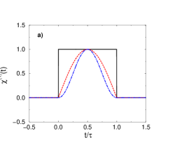
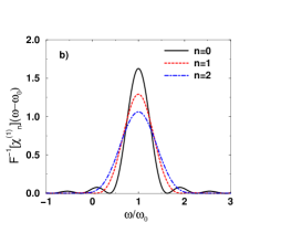
Figure 1: a) Family $\chi_{n}(t)$ of single-pulse aperture functions. The smoothness at the edges increases with in this order: rectangular ($n=0$, continuous line), sine ($n=1$, dashed line), sine-square ($n=2$, dot-dashed line). b) The aperture function in the frequency domain, $F^{-1}[\chi_{n}^{(1)}](\omega-\omega_{0})$, broadens as a result of apodization, with increasing $n$.

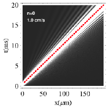
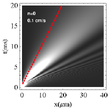
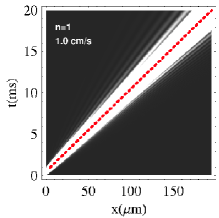
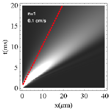
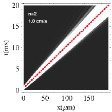
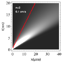
Figure 2: (color online) Spacetime effects of the time-energy uncertainty relation. A pulse of duration $\tau<\top_{0}$ is sped up with respect to the source frequency. The spacetime dynamics is illustrated for a ⁸⁷Rb source with $\tau=1$ms with $\hbar k_{0}/m=1$cm/s (left column, $\top_{0}=0.0467$ms) and $\hbar k_{0}/m=0.1$cm/s (right column, $\top_{0}=4.67$ms), modulated with different apodizing functions to form a single pulse. The dashed line reproduces the classical trajectory. The grey scale changes from dark to light as the function values increase. Figures in the same column show the suppression of the sidelobes in the probability density with increasing $n$.

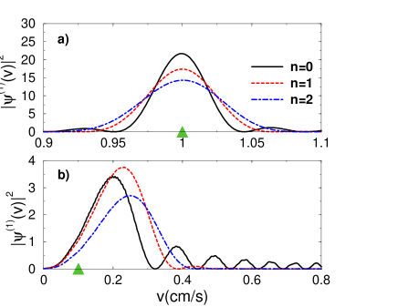
Figure 3: (Color on-line) Distortion of the velocity distribution for pulse duration smaller than $\top_{0}$. The corresponding pulses to Fig. 2 are plotted in velocity space for a ⁸⁷Rb source with $\tau=1$ms apodized with different aperture functions and a) $\hbar k_{0}/m=1$cm/s ($\top_{0}=0.0467$ms) and b) $0.1$cm/s ($\top_{0}=4.67$ms). The triangle marks the classical velocity.

The effect of a short $\tau$ on the energy distribution has already been studied in [2, 28] from which a time-energy uncertainty relation was inferred. Indeed, the uncertainty product reaches an approximate minimum of $2\hbar$ if the pulse duration is shorter than $\top_{0}=\pi/\omega_{0}$. The space-time dynamics for a source apodized with a rectangular aperture function is illustrated in Fig. 2, where it is shown that for $\tau>\top_{0}$ the quantum average of the position operator follows the classical free-particle trajectory whereas if $\tau\lesssim\top_{0}$ the quantum pulse is sped up. Fig. 3 shows for different $\chi_{n}(t)$ ($n=0,1,2$) the effect on the velocity distribution which is only centered at $\hbar k_{0}/m$ for $\tau>\top_{0}$. Concerning the apodization, the higher the value of $n$ the narrower is the mean width of $\chi_{n}(t)$ and the larger the shift on the mean velocity. The smoothing of the $\chi_{n}(t)$ is reflected on the suppression of the sidelobes in the velocity distribution.

3 Smooth switching: apodization and diffraction in time

Instead of forming a finite pulse as discussed in the previous section, some sources are prepared to reach a stationary regime with constant flux after the initial transient. The extreme case is the sudden, zero-time switching of Sec. 1. In this section we shall study how the matter-wave dynamics is modified for slow aperture functions with a given switching time $\tau$. In order to do so, we introduce the family of switching functions

$$\chi^{s}(t)=\cases{0,\qquad t<0\\ \chi(t),\qquad 0\leq t<\tau\\ 1,\qquad t\geq\tau}$$

where it is assumed that $\chi(\tau)=1$, and which is represented in Fig. (4)a for $\chi(t)=\sin^{n}\Omega_{s}t$ with $n=0,1,2$ and $\Omega_{s}=\pi/2\tau$. Note that for $n=0$, one recovers the sudden aperture $\chi_{0}(t)=\Theta(t)$ which maximises the diffraction in time fringes. For $n=1$ (n=2) the source amplitude follows half a sine (square)-lobe. The general result for the time-dependent wavefunction simply reads,

$$\psi_{\chi}^{s}(x,k_{0},t;\tau)=e^{-i\omega_{0}\tau}\psi_{0}\left(x,k_{0},t-\tau\right)\Theta(t-\tau)+\psi^{(1)}_{\chi}(x,k_{0},t;\tau),$$ (10)

where the superscript $s$ stands for ${\it switching}$ and $\psi^{(1)}_{\chi}$ refers to a pulse of length $\tau$ and apodizing function $\chi$.

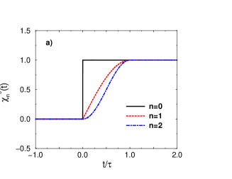
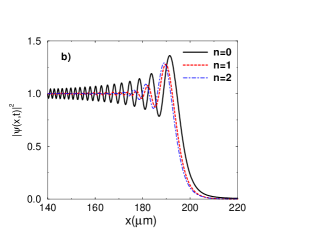
Figure 4: a) Family $\chi_{n}(t)$ of switching-on aperture functions. The smoothness at the edges increases with $n$. b) Apodization of the ⁸⁷Rb beam profiles with increasing smoothness of the aperture function (higher $n$), and fixed switching time $\tau_{s}=0.5$ms at $t=20$ms, and $\hbar k_{0}/m=1$ cm/s.

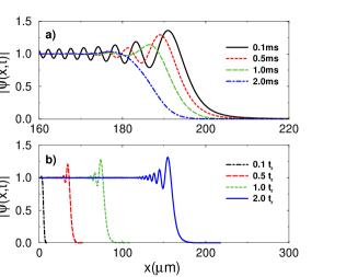
Figure 5: Revival of the diffraction in time. a) The oscillations in the beam profile characteristic of the diffraction in time are gradually suppressed with increasing switching time $\tau$. The beam profile is shown at $t=20$ms, and $\hbar k_{0}/m=1$cm/s. For increasing $\tau$ the amplitude of the oscillations diminishes and the signal is delayed. b) During the time evolution there is a revival of the diffraction in time which is again clearly visible for times greater than $t_{r}=\omega_{0}\tau^{2}$ ($\tau=1$ms, $\hbar k_{0}/m=0.5$cm/s, and $t_{r}=16.8$ms). Both a) and b) refer to a ⁸⁷Rb source which is switched on following a sine-square function.

Figure 4(b) shows the effect of a finite switching time on the oscillatory pattern at a given time. As a result of the smooth aperture functions new frequencies are singled out, leading to a progressive suppression of diffraction in time. Moreover, for a given $\chi_{n}(t)$ function, a larger switching time $\tau$ increases the apodization of the source, washing out the fringes in the probability density, see Fig. 5(a). (In this sense, the effect of a finite band-width source is tantamount to a time dependent modulation, as was shown in [23].) However, it is remarkable that the effect of the apodization is limited in time because of a revival of the diffraction in time. The intuitive explanation is that the intensity of the signal from the apodization “cap”, see Fig. 6, decays with time whereas the intensity of the main signal (coming from the step excitation) remains constant. For sufficiently large times, the main signal, carrying its diffraction-in-time phenomenon, overwhelms the effect of the small cap. One can estimate the revival time by considering that the momentum width of the apodization cap will be of the order

$$\Delta p\approx\sqrt{2m\hbar(\omega_{0}+\Omega_{s})}-\sqrt{2m\hbar(\omega_{0}-\Omega_{s})}\approx\sqrt{2m\hbar\omega_{0}}\frac{\pi}{2\omega_{0}\tau},$$ (11)

and taking into account the, essentially linear with time , spread of the cap half-pulse described by $\psi_{\chi}^{(1)}$ in Eq. (10) (we have checked numerically that the classical dispersion relation $\Delta x(t)\simeq\Delta x(0)+\Delta pt_{r}/m$ holds).

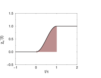
Figure 6: Aperture function decomposition. In a switching proccess the aperture function has a finite transient component responsible for the apodization (shaded area). Such apodization cap is followed by a step excitation for $t\geq\tau$ which leads eventually to the revival of diffraction in time.

The ratio of the spatial widths corresponding to the initial and evolved cap $\psi_{\chi}^{(1)}$ is given by

$$R=\frac{\Delta x(0)}{\Delta x(t_{r})}\approx\frac{\Delta x(0)}{\Delta x(0)+\Delta pt_{r}/m}.$$ (12)

Taking $\Delta x(0)=\sqrt{2\hbar\omega_{0}/m}\tau$ and imposing $R=1/2$ leads to the expression for a revival time scale

$$t_{r}\approx\omega_{0}\tau^{2},$$ (13)

which is analogous to the Rayleigh distance of classical diffraction theory but in the time domain [31]. The smoothing effect of the apodizing cap cannot hold for times much longer than $t_{r}$. This is shown in Fig. 5(b), where the initially apodized beam profile develops eventually spatial fringes, which reach the maximum value associated with the sudden switching at $t\approx 2t_{r}$.

4 Multiple pulses

We show next that the single pulse aperture functions $\chi^{(1)}(t)$, described in section 2 are useful to consider matter wave sources periodically modulated in time. Indeed, the $N$-pulse aperture function can be written as a convolution of $\chi^{(1)}(t)$ with a grating function. In particular, if the grating function $g(t)$ is chosen to be a finite Dirac comb $g_{N}(t)=\sum_{j=0}^{N-1}\delta(t-jT)$, it is readily found that

$$\chi^{(N)}(t)=\chi^{(1)}(t)*g_{N}(t)=\int dt^{\prime}\chi^{(1)}(t-t^{\prime})g_{N}(t^{\prime})=\sum_{j=0}^{N-1}\chi^{(1)}(t-jT),$$ (14)

which describes the formation of $N$ consecutive $\chi^{(1)}$-pulses, each of them of duration $\tau$ and with an “emission rate” (number of pulses per unit time) $1/T$.

If we are to describe an atom beam periodically modulated with such apodizing function, the space-time evolution simply reads,

$$\psi_{\chi}^{(N)}(x,k_{0},t)=\sum_{j=0}^{N-1}e^{-i\omega_{0}jT}\psi_{\chi}^{(1)}(x,k_{0},t-jT;\tau)\Theta(t-jT)$$ (15)

being a linear combination of the single-pulse wavefunction $\psi^{(1)}(x,t)$ studied in section 2. The $\Theta(t-jT)$ corresponds to the condition that the $j$-th pulse starts to emerge only after $jT$.

A similar mathematical framework can be employed to describe an atom laser in the no-interaction limit. The experimental prescription for an atom laser depends on the outcoupling mechanism. Here we shall focus on the scheme described in [12, 13]. The pulses are obtained from a condensate trapped in a MOT, and a well-defined momentum is imparted on each of them at the instant of their creation through a stimulated Raman process. The result is that each of the pulses $\psi_{\chi}^{(1)}$ does not have a memory phase, the wavefunction describing the coherent atom laser being then

$$\phi_{\chi}^{(N)}(x,k_{0},t)=\sum_{j=0}^{N-1}\psi_{\chi}^{(1)}(x,k_{0},t-jT;\tau)\Theta(t-jT),$$ (16)

compare with (15).

Figure 7: Beam density profile of a ²³Na atom laser with $\tau=0.833ms$, $T=0.3ms$, in the coherently constructive $\omega_{0}T=10\pi$ ($5.9$ cm/s) (a), destructive $\omega_{0}T=11\pi$ ($5.9$ cm/s) (b), and incoherent case (c), with same conditions than a) with a sine-square aperture function. The conditions equivalent to the experiment reported in [12] ($\tau=0.83$ms, $T=0.05$ms) are studied for the constructive (d), destructive (e) and incoherent case (f). If the pulse is not apodized the beam profile becomes noisy as shown in (g) for rectangular $\chi$, in the same conditions than (d). In all cases the norm is relative to the incoherent case.

It is interesting to impose a relation between the outcoupling period $T$ and the kinetic energy imparted to each pulse $\hbar\omega_{0}$, such that $\omega_{0}T=l\pi$, where if $l$ is chosen an even (odd) integer the interference in the beam profile $\psi_{\chi}^{(N)}$ is constructive (destructive), see Fig. 7. However, in the case of a periodically chopped atom beam $\psi_{\chi}^{(N)}$, Eq. (15), the additional phase $e^{-i\omega_{0}jT}$ singles out the constructive interference independently of the parity of $l$.

So far we have assumed that the source is coherent. The interference pattern between adjacent pulses is affected by the presence of noise in the phases [32]. The average over many realisations in which the phase $\alpha_{j}$ of each pulse varies randomly in $[0,2\pi]$ leads to the density profile,

$$\rho(x,t)=\left\langle\left|\sum_{j=0}^{N-1}e^{i\alpha_{j}}\psi_{\chi}^{(1)}(x,k_{0},t-jT;\tau)\Theta(t-jT)\right|^{2}\right\rangle_{\alpha}$$ (17)

which reproduces the incoherent sum of the pulses, $\rho(x,t)=\sum_{j}|\psi_{n}^{(1)}(x,k_{0},t-jT;\tau)|^{2}\Theta(t-jT)$.

One advantage of employing stimulated Raman pulses is that any desired fraction of atoms can be extracted from the condensate. Let us define $s$ as the number of atoms outcoupled in a single pulse, $\psi^{(1)}_{\chi}$. The total norm for the $N$-pulse incoherent atom laser is simply $\mathcal{N}_{inc}=sN$. A remarkable fact for coherent sources is that the total number of atoms $\mathcal{N}_{c}$ outcoupled from the Bose-Einstein condensate reservoir depends on the nature of the interference [33]. Therefore, in Figs 7 and 8 we shall consider the signal relative to the incoherent case, namely, $|\psi^{(N)}_{\chi}|^{2}/\mathcal{N}_{inc}$.

Note the difference in the time evolution between coherently constructive and incoherent beams in Fig. 8:

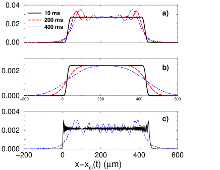
Figure 8: Time evolution of a ²³Na atom laser beam modulated by a sine-square function with $\tau=0.833$ms, $T=0.05$ms, moving at $5.9$cm/s in the a) coherently constructive, b) incoherent case, and c) rectangular single pulse approximation to a) (the snapshot at $t=200$ms is omitted for clarity). Note that $x_{cl}=\hbar k_{0}t/m$ is the classical trajectory. In all cases the norm is relative to the incoherent case, see (17) and the paragraph bellow.

At short times both present a desirable saturation in the probability density of the beam. However, in the former case a revival of the diffraction in time phenomena takes place in a time scale $\omega_{0}\tau^{2}$, similar to the smooth switching considered in section 3, whereas the later develops a bell-shape profile.

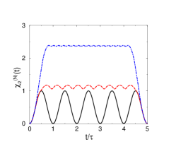
Figure 9: (color online) Many-pulse aperture function $\chi_{2}^{(N)}(t)$ with $\tau_{eff}=5\tau$ and increasing number of pulses N: 5, (solid line), 10 (dashed line), and 20 (dot-dashed line). In the highly overlapping regime $\chi_{2}^{(N)}(t)$ can be approximated by a a single pulse rectangular aperture function of duration $\tau_{eff}=(N-1)T+\tau$.

Interestingly, whenever the overlap amongst different pulses is coherently constructive or with phase memory (as in the periodic chopping of a beam), an effective single-pulse aperture function can be introduced. Indeed, if $\tau/T\gg 1$ as in the actual experiments [12, 13], it follows that $\chi_{eff}(t)=\sum_{j=1}^{N-1}\chi(t-jT)\propto\Theta(t)\Theta(\tau_{eff}-t)$ for any $\chi$, where the effective pulse duration is $\tau_{eff}=(N-1)T+\tau$. More precisely it reaches a plateau in the time interval $[\tau,nT-\tau]$ but has both a front and a back cap of duration $\tau$ associated with the switching on and off. This is graphically illustrated in Fig. 9 for $\chi_{2}^{(N)}(t)$, describing the formation of $N$ pulses with a sine-square modulation $\chi_{2}^{(1)}(t)$. Moreover, the quality of this approximation improves as the time of evolution becomes greater than the revival time, see Fig 8(c). Clearly this is only valid in the highly-overlapping regime whereas if the overlap is restricted to few pulses no saturation of the beam profile is observed. This is an important simplification to optimise the aperture function and design the beam profile of an atom laser.

5 Discussion

We have studied the dynamics of non-interacting boson sources which are modulated in time with arbitrary aperture functions. Starting with different switching-on procedures we have accounted first for single pulse formation and systematically described the multiple pulse case. Whenever the modulation is sudden, the spreading of the source exhibits oscillation in the density profile, which is the taletelling sign of the quantum diffraction in time phenomenon. For apodized sources with smooth aperture functions the oscillations are suppressed, thus bringing to the quantum domain the classical apodization techniques usual in signal analysis and Fourier optics. However, for long or multiple overlapping pulses the smoothing is limited by a time scale $t_{r}$, associated with a revival of the diffraction-in-time phenomenon. Multiple pulse formation has been examined for different possible cases. For constructive or for random averaged phases, a saturation effect occurs providing a flat intensity profile before $t_{r}$, which later develops spatial fringes and a bell-shape profile respectively. For both types of beam formation the initial flat beam region is smooth for apodized pulses but noisy for square ones. While these results are already quite relevant for an understanding of pulse formation and intended applications of the atom laser, the next natural step will be to extend the present analysis to systems with atom-atom interaction.

Appendix A The Moshinsky function

The Moshinsky function can be related to the Faddeyeva $w(z)$ and complementary error function [34, 35],

$$M(x,k,\tau):=\frac{e^{i\frac{x^{2}}{2\tau}}}{2}w(-z),\qquad{\rm where}\qquad z=\frac{1+i}{2}\sqrt{\tau}\left(k-\frac{x}{\tau}\right),$$ (18)

and $w(z)$ is defined as

$$w(z):=e^{-z^{2}}{\rm{erfc}}(-iz)=\frac{1}{i\pi}\int_{\Gamma_{-}}du\frac{e^{-u^{2}}}{u-z},$$ (19)

$\Gamma_{-}$ being a contour in the complex $z$-plane which goes from $-\infty$ to $\infty$ passing below the pole.

Appendix B Arbitrary aperture function

In what follows we will be interested in pulses modulated with an arbitrary aperture function $\chi(t)$ which is zero outside the interval $[0,\tau]$. An analytical result can be obtained in such case by means of Fourier series. Noting that

$$\chi(t)=\sum_{r=-\infty}^{\infty}c_{r}e^{i\frac{2\pi rt}{\tau}}\Theta(t)\Theta(\tau-t)\quad{\rm with}\qquad c_{r}=\frac{1}{\tau}\int_{0}^{\tau}\chi(t)e^{-i\frac{2\pi rt}{\tau}}dt,$$ (20)

the wavefunction at the origin can be conveniently written for all times as an infinite series

$$\psi_{\chi}(x=0,k_{0},t)=\sum_{r=-\infty}^{\infty}c_{r}e^{-i\left(\omega_{0}+\frac{2\pi rt}{\tau}\right)t}\Theta(t)\Theta(\tau-t)=\sum_{r=-\infty}^{\infty}c_{r}e^{-i\omega_{r}t}\Theta(t)\Theta(\tau-t),$$ (21)

which evolves for $x,t>0$ as

$$\psi_{\chi}(x,k_{0},t;\tau) = \sum_{r=-\infty}^{\infty}c_{r}\psi_{0}^{(1)}(x,k_{r},t;\tau)$$ (22)

where

$$\psi_{0}^{(1)}(x,k_{r},t;\tau)=\psi_{0}\left(x,k_{r},t\right)-\Theta(t-\tau)e^{-i\omega_{r}\tau}\psi_{0}\left(x,k_{r},t-\tau\right)$$ (23)

and $\hbar k_{r}=\sqrt{2m\hbar\omega_{r}}$, with the branch cut taken along the negative imaginary axis of $\omega_{r}=\omega_{0}+2\pi r/T$. This is an amusing expression for it relates the dynamics of a source with an arbitrary aperture function with that of rectangular pulses of different coherent sources. As a caveat, less general decompositions may be simpler as in the $\chi_{1}^{(1)}(t)$ case discussed in section 2.

References

References

- [1] Moshinsky M 1952 Phys. Rev. 88 625
- [2] Moshinsky M 1976 Am. Jour. Phys. 44 1037
- [3] Kleber M 1994 Phys. Rep. 236 331
- [4] García-Calderón G and Villavicencio J 2001 Phys. Rev. A 64 012107
- [5] Granot E and Marchewka A 2005 Europhys. Lett. 72 341
- [6] del Campo A and Muga J G 2006 Europhys. Lett. 74, 965
- [7] del Campo A, Delgado F, García-Calderón G, Muga J G and Raizen M G 2006 Phys. Rev. A 74 013605
- [8] Hils T, Felber J, Gähler R, Gläser W, Golub R, Habicht K and Wille P 1998 Phys. Rev. A 58 4784
- [9] Steane A, Szriftgiser P, Desbiolles P and Dalibard J 1995 Phys. Rev. Lett. 74 4972; Arndt M, Szriftgiser P, Dalibard J, and Steane A M 1996 Phys. Rev. A 53 3369; Arndt M, Szriftgiser P, Dalibard J, and Steane A M 1996 Phys. Rev. A 53 3369
- [10] Lindner F et al. 2005 Phys. Rev. Lett. 95 040401
- [11] Colombe Y, Mercier B, Perrin H, and Lorent V 2005 Phys. Rev. A 72 061601(R)
- [12] Hagley E W et al. 1999 Science 283 1706
- [13] Trippenbach M. 2000 J. Phys. B 33 47
- [14] Mewes M O et al. 1997 Phys. Rev. Lett. 78 582
- [15] Carpentier A V, Michinel H, Rodas-Verde M I, and Pérez-García V I 2006 Phys. Rev. A 74 013619
- [16] Köhl M, Busch T, Molmer K, Hänsch T W, Esslinger T 2005 Phys. Rev. A 72 063618
- [17] Riou J-F, Guerin W, Le Coq Y, Fauquembergue M, Josse V, Bouyer P, and Aspect A 2006 Phys. Rev. Lett. 96 070404
- [18] Kramer T and Pinilla M 2006 Phys. Rev. A 74 013611
- [19] Fowles G R 1968 Introduction to modern optics (New York: Dover)
- [20] Blackman R B and Tukey J W 1959 The measurement of power spectra from the point of view of communications engineering (New York: Dover)
- [21] Guerin W et al. Preprint cond-mat/0607438
- [22] Büttiker M and Thomas H 1998 Superlatt. Microstruct. 23 781
- [23] Muga J G and Büttiker M 2000 Phys. Rev. A 62 023808
- [24] Muga J G, Sala R and Egusquiza I 2002 Time in Quantum Mechanics, (Berlin: Springer)
- [25] Gähler R and Golub R 1984 Z. Phys. B 56 5
- [26] Felber J, Gähler R and Golub R 1988 Physica B 151 135
- [27] Brukner C and Zeilinger A 1997 Phys. Rev. A 56 3804
- [28] del Campo A and Muga J G 2005 J. Phys. A: Math. Gen. 38 9803
- [29] Baute A D, Egusquiza I L and Muga J G 2001 J. Phys. A 34 4289
- [30] del Campo A and Muga J G 2006 J. Phys. A: Math. Gen. 39, 5897
- [31] Brooker G 2003 Modern classical optics (New York: Oxford)
- [32] Vainio O et al. 2006 Phys. Rev. A 73 063613
- [33] Hagley E W et al 1999 Phys. Rev. Lett. 83 3112
- [34] Faddeyeva V N and Terentev N M 1961 Mathematical Tables: Tables of the values of the function for complex argument (New York: Pergamon)
- [35] Abramowitz A and Stegun I A 1965 Handbook of Mathematical Functions (New York: Dover)