Are Domain Walls in 2D Spin Glasses described by Stochastic Loewner Evolutions?

Abstract

Domain walls for spin glasses are believed to be scale invariant; a stronger symmetry, conformal invariance, has the potential to hold. The statistics of zero-temperature Ising spin glass domain walls in two dimensions are used to test the hypothesis that these domain walls are described by a Schramm-Loewner evolution $\mathrm{SLE}_{\kappa}$. Multiple tests are consistent with $\mathrm{SLE}_{\kappa}$, where $\kappa=2.32\pm 0.08$. Both conformal invariance and the domain Markov property are tested. The latter does not hold in small systems, but detailed numerical evidence suggests that it holds in the continuum limit.

The geometrical characterization of physical objects is central to much of our understanding of their energetics and dynamics. The relevant geometries can be as simple as points or gently curved surfaces. Many objects are not well-described by an integer dimension, but have a scale-dependent measure that can be represented by a fractal dimension. For example, continuous phase transitions in homogeneous systems have nonanalytic behavior consistent with fractal dimensions for the surfaces that separate phases. Evidence for fractal domain walls is seen in scattering experiments and numerical simulations. In models of glassy systems with quenched disorder (frozen-in random fields), analytic work and numerical simulations indicate that domain walls can be scale-invariant and fractal at low temperatures. In two-dimensional homogeneous systems, the additional symmetry of conformal invariance often applies and yields detailed predictions for critical exponents, the effects of boundary conditions, and a background for physical explanations.

The conjunction of conformal invariance with the presence of a domain Markov property (DMP) in statistical mechanics models has led to an even more complete - and in several cases mathematically rigorous - description of fractal curves such as loop-erased self-avoiding walks, percolation hulls, and domain walls at phase transitions in two dimensions in the scaling (i.e., continuum) limit CardyReview ; BauerBernard . Schramm showed that when both properties are present the probability measure on these curves is described by a Schramm-Loewner evolution $\mathrm{SLE}_{\kappa}$ schramm . Random sequences of simple conformal maps can be used to generate the fractal curves with the correct measure, if the real-valued driving function that underlies the maps is a Brownian motion. The diffusion coefficient $\kappa$ of the Brownian motion uniquely parameterizes the process and is related to the fractal dimension of the curve via $d_{f}=1+\kappa/8$. This deep connection has led to very precise characterization of these curves for pure systems such as $q$-states Potts model, $O(n)$ models and percolation.

An outstanding question is whether SLE can be applied to other systems. Numerical evidence has been presented, for example, that SLE describes certain isolines in 2D turbulence BernardFalkovichEtc . The broad question of whether and how conformal invariance, a necessary condition for SLE, applies to disordered systems is still very much open. Attempts to extend the apparatus of conformal field theory to systems with quenched disorder, a notably difficult subject cardy , have suggested some numerical tests, such as finite size scaling jacobsen . A positive result was obtained recently for surface wavefunction multifractality at the 2D localization transition with spin-orbit symmetry gruzberg . Most importantly for our work, Amoruso, Hartmann, Hastings and Moore amoruso have suggested that domain walls in the 2D spin glass have conformal invariance.

Here we directly investigate whether the domain wall statistics converges to an $\mathrm{SLE}_{\kappa}$. We apply several tests. We examine the winding of domain wall around a cylinder, as well as the angular distribution of the curves and the dipolar SLE hitting probability. We use an iterated slit map (discretized inverse Loewner evolution) to determine the driving function and test whether it converges to Brownian motion. We directly test the DMP by comparing precise domain wall statistics in “whole” and “cut” domains. To determine the significance of these tests, we carry out the same analyses for the loop-erased random walk (LERW), which has $\mathrm{SLE}_{2}$ as a scaling limit, and for paths on minimal spanning trees (MST), which are not conformally invariant Wilson . We find that, for one choice of boundary conditions (BCs), the spin glass domain wall passes all tests with a consistent value of $\kappa$.

We study the domain walls in a 2D Ising spin glass with Gaussian disorder. We use the Edwards-Anderson Hamiltonian ${\cal H}=-\sum_{\langle ij\rangle}J_{ij}s_{i}s_{j}$, where $s_{i}=\pm 1$ and the $J_{ij}$ are each chosen from a Gaussian distribution with zero mean. The glass transition is at $T=0$; we study the minimum energy states at $T=0$ using an exact optimization algorithm Barahona and sample over disorder realizations. There are two ground states, connected by a global spin flip, in any finite sample. In the scaling picture based on domain walls and droplets, introduced by McMillan mcmillan , Bray and Moore BrayMoore , and Fisher and Huse fisherhuse , there are two ground states in the thermodynamic limit middleton ; youngpalassini . Domain walls (DWs) separate these two ground states. The domain wall energy scales as $E_{{\rm DW}}\sim L^{\theta}$ mcmillan ; BrayMoore ; fisherhuse for DWs defined at scale $L$, with $\theta=-0.28(1)$.

We work on a triangular lattice that has $W$ spins in each of $L$ rows, as sketched in Fig. 1. Our samples are cylindrical, with periodic rows. One can uniquely describe ground state pairs by the bond satisfactions $\sigma_{ij}={\rm sgn}(J_{ij}s_{i}s_{j})$, where $\Pi_{\Delta}\sigma_{ij}={\rm sgn}(\Pi_{\Delta}J_{ij})$ for any elementary triangle $\Delta$. Periodic BCs result from fixing $\Pi_{(ij)\in p_{\alpha}}\sigma_{ij}=\Pi_{(ij)\in p_{\alpha}}{\rm sgn}(J_{ij})$, where $p_{\alpha}$ are the sets of boundary bonds on the upper ($\alpha=1$) and lower ($\alpha=2$) edges BCs. Imposing $\Pi_{(ij)\in p_{\alpha}}\sigma_{ij}=-\Pi_{(ij)\in p_{\alpha}}{\rm sgn}(J_{ij})$ gives antiperiodic BCs (equivalent to a change in the sign of the $J_{ij}$ along a column of bonds). Comparing ground states for periodic and antiperiodic BCs gives a domain wall: a simple path on the dual lattice that crosses bonds whose satisfaction differs between the two BCs. A domain wall is the minimizer of the cost function $2\sum_{(ij)\in\gamma}F_{ij}$, with $F_{ij}=J_{ij}s_{i}^{0}s_{j}^{0}$ and $s_{i}^{0}$ the spins in the periodic ground state, over open paths $\gamma$ from the bottom to the top of the cylinder. In the ground state, the cost of any closed loop is positive footnote1 .

We refer to the domain wall found using this particular periodic-antiperiodic BC comparison as “floating” (F-PA), as the endpoints of the domain wall are not fixed. We also consider a periodic-antiperiodic BC change where the domain wall at one end is locally constrained to a single chosen bond on the lower boundary (L-PA), i.e., a given $\sigma_{ij}$ is reversed on the lower boundary.

The choice of $L$ and $W$ give the cylinder shape, with the circumference given by $X=W$ and the length by $Y=(\sqrt{3}/2)L$. We find that the averages converge for $W\geq 4L$. The results for the first quarter of the path for $W=L$ agree with those for $W\gg L$, within our accuracy. For comparison, we also study LERW curves and paths between two points in the MST, both on honeycomb lattices; LERW curves have dimension $d_{f}=5/4$ in the continuum limit and MST paths appear to have a fractal dimension $d_{f}=1.217(3)$ MST .

We estimate $d_{f}$ for the domain wall by computing the mean total path length $\overline{S}(L)$ of the domain wall, comparing with $\overline{S}(L)\sim L^{d_{f}}$, the overline indicating averages over $\approx 10^{4}$ samples at sizes up $5\times 10^{5}$ spins, and also by computing the sample averaged distance from the origin as a function of partial path length. We find $d_{f}=1.28(1)$, in statistical agreement with previous work SG2D , for both F-PA and L-PA BC’s.

We test conformal invariance and consistency with the SLE description by measuring the winding of the F-PA domain wall around a long cylinders with $Y\gg X$. The prediction from SLE is that the variance of the transverse displacement $x$ of the end point from the starting location is $\langle x^{2}\rangle=\frac{4}{\pi}(d_{f}-1)XY$. We studied cylinders with $8\leq W\leq 32$ and up to $L=800$ for at least $10^{4}$ samples at each of at least eight values of $L$. Our data is consistent with $\frac{\pi}{4}\langle x^{2}\rangle$ linear in $XY$, with a coefficient of $0.27\pm 0.01$ for $L>4W$, in agreement with conformal invariance, again for both F-PA and L-PA BC’s.

A powerful result schramm2 from SLE is a prediction of the probability that a curve generated by SLE will pass to the left of a given point at polar coordinates $(R,\phi)$ (see Fig. 1 for notation). Given scale invariance, the probability that the curve passes to the left of $(R,\phi)$ depends only on $\phi$, and the theory of SLE can be used to predict schramm2

$$P_{\kappa}(\phi)=\frac{1}{2}+\frac{\Gamma\left(\frac{4}{\kappa}\right)}{\sqrt{\pi}\Gamma\left(\frac{8-\kappa}{2\kappa}\right)}\tan(\phi)F_{12}\left(\frac{1}{2};\frac{4}{\kappa},\frac{3}{2};-\tan^{2}(\phi)\right)\,,$$ (1)

where $F_{12}$ is the hypergeometric function and $\kappa$ is the diffusion parameter from continuum SLE. Our results (Fig. 1) for $P(\phi)$ depend on the choice of BC. For F-PA BCs the measured $P(\phi)$ is most consistent with the analytical form in the range $\kappa_{{\rm eff}}^{F}=2.32\pm 0.08$, consistent with the relation $\kappa=8(d_{f}-1)$. For L-PA domain walls measured from the fixed end, we find $\kappa_{{\rm eff}}^{L}=2.85\pm 0.10$. We find the same two BC-dependent values tobepub using another test: a comparison of the distribution for the displacement between the DW endpoints with the form predicted using dipolar SLE dipolar , which describes the limit $X/Y\rightarrow\infty$ for SLE curves that start at a given point $a$ and terminate on the upper boundary. Constraining the domain wall to start at a given point (L-PA BCs) rather than choosing domain walls that start at a point (i.e., conditioning on $a$) with F-PA BCs changes the effective $\kappa$. Domain walls with fixed endpoints are not consistently described by $\mathrm{SLE}_{\kappa}$ over their entire length.

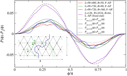
Figure 1: Plots of $P(\phi,R)-P_{2}(\phi)$, where $P(\phi,R)$ is the probability for the domain wall to pass to the left of a point with polar coordinates $(R,\phi)$ (see inset). The magnitude of statistical errors (not shown) is consistent with the apparent fluctuations of the data lines. The predicted $P_{2}(\phi)=[\phi-\frac{1}{2}\sin(2\phi)]/\pi$ for $\kappa=2$ is subtracted to display small variations clearly. The data from F-PA paths agrees with SLE predictions for $\kappa$ in the range $2.24<\kappa<2.40$, while L-PA paths give $\kappa\approx 2.85(10)$. Inset: A domain wall of length $S=9$ in a sample with $L=4$ rows and $W=6$ columns.

The boundary conditions appear not to affect the fractal dimension, but clearly do affect more subtle aspects of the geometry. A similar result holds for the LERW: absorbing and reflecting boundary conditions both are consistent with $d_{f}=\frac{5}{4}$ BauerBernard , but $P(\phi)$ is well fit by Eq. (1) with $\kappa=2$ for absorbing BCs, as expected, in contrast with $P(\phi)\approx\phi/\pi$ for reflecting BCs.

Note that the L-PA DW energy approaches a constant as $L\rightarrow\infty$, in contrast with $E_{{\rm DW}}\sim L^{\theta}$ for F-PA DWs. This difference holds in general for $\theta\leq 0$, as can be seen by summing L-PA domain wall energies defined over geometrically increasing scales connecting the localized region to the large scale. Essentially, the L-PA constraint gives an $O(1)$ correction to $E_{{\rm DW}}$ from the cost of the single bond at the localized end. Apparently, the optimization over successive scales distorts the curve from the form expected from SLE, while optimization over a single global scale gives results consistent with SLE.

To more carefully inspect the correspondence with SLE, we have used a discrete Loewner evolution to map the domain walls, represented by sequences of points $z_{i}^{0}=x_{i}^{0}+iy_{i}^{0}$, $i=1\ldots S$, in the complex half-plane, onto a real-valued sequence $\xi(t_{i})$ defined at discrete $t_{i}$ and studied the sample statistics and correlations of the interpolated $\xi(t)$. For continuous curves generated by SLE, the underlying function $\xi(t)$ is Brownian motion with diffusion constant $\kappa$. The sequence is initialized by setting $t_{0}=0$ and $\xi(t_{0})=0$. We then recursively map the sequence $\{z_{i}^{i-1},\ldots,z_{S}^{i-1}\}$ to the transformed and shortened sequence $\{z_{i+1}^{i},\ldots,z_{S}^{i}\}$ using the map appropriate for dipolar SLE (first defining $\Delta_{i}=\pi y_{i}^{i}/2Y$),

$$t_{i} = t_{i-1}-2(Y/\pi)^{2}\log[\cos(\Delta_{i})]\ \ ;\ \ \xi(t_{i})=x_{i}^{i-1}$$ (2)

$$z_{j}^{i} = \xi(t_{i})+\frac{2L}{\pi}\cosh^{-1}\left\{\cosh\left[\frac{\pi(z-\xi_{i})}{2L}\right]/\cos(\Delta_{i})\right\}.$$

These maps are a sequence of slit maps that successively remove the first point from the sequence (see Fig. 2) and maintain the hydrodynamic normalization used in SLE.

The simplest test for the diffusive property of $\xi(t)$ is to examine its distribution at fixed times. Our data for $L^{2}/5\gtrsim t\gtrsim 50$ are consistent with a Gaussian distribution for $\xi(t)$ with variance $\overline{\xi^{2}(t)}=\kappa_{{\rm eff}}t$ (Fig. 2). We have confirmed that higher cumulants satisfy $\overline{\xi^{2n}(t)}=(2n)!!\left(\overline{\xi^{2}(t)}\right)^{n}$ for $n=2,3,4$, within numerical error, for the same range of $t$. For computations of $\xi(t)$ that start from a free end of a domain wall (F-PA boundary conditions or the free end of L-PA BCs), we find $\kappa_{{\rm eff}}^{F}=2.24\pm 0.08$, while for computations starting from the localized end with L-PA BCs, we estimate $\kappa_{{\rm eff}}^{L}\approx 2.85\pm 0.1$, consistent with our estimates from $P(\phi,R)$. We note that $\xi^{2}(t)$ is also nearly linear in time for paths on the MST, even though such paths are not conformally invariant, but the coefficient is not consistent with the fractal dimension (see Wilson for MST winding angle results).

We have also tested the Markovian property for $\xi(t)$, i.e., that the changes in $\xi(t)$ depend only on the current value of $\xi(t)$ and not on previous values. We studied the correlation function $C_{d}(n)=\langle[\xi(t_{i+n+1})-\xi(t_{i+n})][\xi(t_{i+1})-\xi(t_{i})]\rangle$ at intermediate times; it decays rapidly (by a factor of $\approx 100$ over the range $n=2$ to $n=8$) for both the spin glass and for the LERW tobepub . Note that there must be short term correlations in $\xi(t)$ on the lattice, as there are forbidden sequences of “turns” for the domain wall.

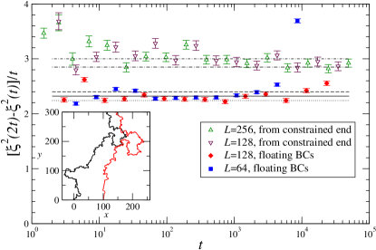
Figure 2: Plot of an effective diffusion constant $\kappa_{{\rm eff}}=\overline{\xi^{2}(2t)-\xi^{2}(t)}/t$, for $W\geq 4L$. Lines indicate $\kappa=2.24$, 2.32, 2.40, 2.85, and 3.00. The range $2.24<\kappa<2.40$ fits the data for curves with F-AP BCs, while $2.85<\kappa<3.00$ describes the diffusion measured from a constrained domain wall end. Inset: Part of a sample conversion of a domain wall in the 2D Ising spin glass to a sequence $\xi(t_{i})$, $i=1\ldots S$. The left curve is the initial domain wall with $\xi(0)=0$, while the red [lighter] curve is the remainder after $500$ applications of the dipolar map, giving $\xi(t_{500}\approx 7239.4)\approx 101.5$.

Given that the Ising spin glass DW passes several SLE tests one must examine the domain Markov property (DMP) in a disordered system. Let us call $P_{D}(\gamma_{ab})$ the probability that the DW happens to coincide with the curve $\gamma_{ab}$ in a domain $D$ (where $a$,$b$ are two given boundary points). The DMP footnote0 states that if one conditions this probability on a piece $\gamma_{ac}$ of the curve, then the probability for the rest of the curve $\gamma_{cb}$ is identical to the original probability on the cut domain $D\setminus\gamma_{ac}$ conditioned on curves starting at $c$, i.e:

$$P_{D}(\gamma_{cb}|\gamma_{ac})=P_{D\setminus\gamma_{ac}}(\gamma_{cb}|c)$$ (3)

Cutting the domain removes bonds that cross the segment $\gamma_{ac}$. In pure statistical systems Eq. 3 is an identity, given proper BCs. One can easily check that the DMP holds in a single realization of disorder. However this property does not survive disorder averaging (as conditioned probabilities are ratio of probabilities) except for percolation $\mathrm{SLE}_{\kappa=6}$ (because of locality).

To evaluate the deviations from the DMP we have computed numerically the ratio of sums of the two probabilities in Eq. (3). We generate domain walls in both whole cylinders and in cylinders cut by all paths $\gamma_{1}$ of a chosen path length $s_{1}$. We sample at least $3\times 10^{7}$ disorder configurations to estimate the ratio $r(\gamma_{1},\gamma_{2})=\sum_{\gamma_{bc}\supset\gamma_{2}}P_{D\setminus\gamma_{1}}(\gamma_{bc}|c)/\sum_{\gamma_{bc}\supset\gamma_{2}}P_{D}(\gamma_{bc}|\gamma_{1})$, with $\gamma_{1}$ starting at the lower boundary, $\gamma_{2}$ a subpath of $\gamma_{bc}$ of path length $s_{2}$, and $\gamma_{1}$ connecting to $\gamma_{2}$ at $c$. If DMP holds strictly, $r(\gamma_{1},\gamma_{2})\equiv 1$. We summarize our data in Fig. 3, where we plot the cumulative probability $C(x)=\sum_{\gamma 1,\gamma_{2}|r(\gamma_{1},\gamma_{2})<x}P_{D}(\gamma_{1},\gamma_{2})$ that $r$ is less than $x$. We find that in small samples with $L=8$, $r$ is statistically distinct from unity for larger $|\gamma_{2}|$. The largest deviations are seen for $\gamma_{2}$ near to and parallel to $\gamma_{1}$. For comparison, we show results of the same analysis for the LERW with both absorbing BCs (A-LERW), where $r$ is unity within statistical error, and for reflecting BCs (R-LERW), where $r$ clearly deviates from unity. In ISG simulations, $C(x)$ is quite close to the curve for A-LERW. Our data cannot rule out the possibility of DMP holding in the continuum limit.

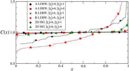
Figure 3: Plot of $C(x)$, cumulative probability of ranked values for $r(\gamma_{1},\gamma_{2})$, as defined in the text. Large deviations from $r=1$, as clearly seen for R-LERW, indicate a failure of the domain Markov property.

It is tempting to conjecture that the emergence of the DMP in the continuum limit follows from the existence of “principal” minimizers, separated from each other on a scale $L$. These are the basins of attraction for minimizing paths: if the start of a DW is displaced from the minimizer’s start by a scale $\ell<L$, the DW merges with principal minimizer within a distance of order $\ell$ middleton . These minimizers are a result of finding shortest paths in a graph with negative weights (but no negative weight loops). In particular, this implies the same statistics for the L-PA and F-PA BCs on a long cylinder. In a broad strip ($X\gg Y$), the differences between L-PA and F-PA BCs must be related to the approach of the constrained path to the principal minimizer over a sequence of scales. Unlike local minimizers, principal minimizers are independent of the direction in which they are traversed. We expect that bulk segments of the L-PA curves are well described locally by $\mathrm{SLE}_{\kappa}$. The conditioning of paths used in defining the DMP may be related to the properties of the minimizing paths footnoteproof . We also note that the LERW with reflecting BCs passes the same set of tests of conformal invariance as the L-PA 2DISG and fails the same set of tests of $\mathrm{SLE}_{\kappa}$.

In conclusion, we have numerically sampled over geometric objects in a system with disorder, domain walls in the 2D Ising spin glass, and tested their statistical geometric properties. We find that the domain walls pass to the left of a given point with probabilty consistent with SLE, wind around long cylinders in a manner consistent with conformal invariance, and that the sequences of conformal maps that generate DWs, i.e., Loewner evolutions $\xi(t)$, give a diffusion constant $\kappa=2.32\pm 0.08$ in accord with a fractal dimension $d_{f}=1.28\pm 0.01$. We directly study the domain Markov property: it fails in small systems, but we can not rule it out in larger systems. This set of tests, whose utility is validated by application to curves in LERW and MST, provides strong numerical support for a description of spin-glass domain walls with unconstrained endpoints by SLE, implying both conformal invariance and a domain Markov property on long scales. Domain walls starting from a localized bond are not consistent with the simplest form of SLE, though more complex conformally invariant descriptions, e.g., SLE with drift such as $\mathrm{SLE}_{\kappa;\rho}$ should be investigated.

We thank M. Biskup, M. Bauer, J. Cardy, C. Newman, A. Ludwig, K. Wiese, and T. Witten and especially M. Hastings for discussions and the authors of Ref. amoruso for sharing their unpublished work. This work was supported in part by NSF grants DMR 0219292, 0606424, and ANR blan06-3-134462 and blan05-0099-01. We thank the KITP (NSF PHY99-07949) and the MPI-PKS for their hospitality.

References

- (1) J. Cardy, Ann. Phys. 318, 81 (2005).
- (2) M. Bauer and D. Bernard, Phys. Rep. 432, 115 (2006).
- (3) O. Schramm, Israel J. Math. 128 221 (2000).
- (4) D. Bernard et al, Nature Physics 2 124 (2006).
- (5) J. Cardy cond-mat/9911024; in Statistical Field Theories, A. Cappelli and G. Mussardo eds, Kluwer, (2002) cond-mat/0111031; V. Gurarie and A. W. W. Ludwig, J. Phys. A 35, L377 (2002); D. Bernard, cond-mat/9509137.
- (6) J. Cardy and J. Jacobsen, Phys. Rev. Letters, 79, 4063 (1997).
- (7) H. Obuse et al., cond-mat/0609161
- (8) C. Amoruso, A. K. Hartmann, M. B. Hastings, and M. A. Moore, cond-mat/0601711.
- (9) We quote our results, consistent with, e.g., M. Cieplak, A. Maritan, J. R. Banavar, Phys. Rev. Lett. 72 2320 (1994); R. Dobrin and P. M. Duxbury, Phys. Rev. Lett. 86 5076 (2001); and Wilson .
- (10) D. B. Wilson, Phys. Rev E 69, 037105 (2004); B. Wieland and D. B. Wilson, Phys. Rev. E 68, 056101 (2003).
- (11) See, e.g., H. Rieger et al, J. Phys. A 29, 39 (1996).
- (12) F. Barahona, J. Phys. A 15, 3241 (1982).
- (13) W. L. McMillan, J. Phys. C 17, 3179 (1984).
- (14) A. J. Bray and M. A. Moore, in Heidelberg Colloquium on Glassy Dynamics, van Hemmen and Morgenstern, eds., Springer (Berlin, 1986).
- (15) D. S. Fisher and D. A. Huse, Phys. Rev. B 38, 386 (1988); J. Phys. A 20, L1005 (1987).
- (16) A. A. Middleton, Phys. Rev. Lett. 83, 1672 (1999).
- (17) M. Palassini and A. P. Young, Phys. Rev. Lett. 83, 5129 (1999).
- (18) This is consistent with and zero double points on the domain wall in the large scale limit.
- (19) O. Schramm, Elec. Comm. Prob. 6 115 (2001). This formula holds for SLE in the upper half plane, but should describe SLE curves near their start here. Our results are independent of , for .
- (20) A. A. Middleton, D. Bernard, P. Le Doussal, in preparation.
- (21) M. Bauer, D. Bernard, J. Houdayer, J. Stat. Mech. P03001 (2005).
- (22) Compared to standard SLE, the formulation of the domain Markov property is modified for the case where the starting point of the curve is not imposed. Eq. 3 is consistent with probabilities for curves conditioned to start at a given point defined by dipolar SLE.
- (23) Conditioning upon reveals an interesting stability property of minimizers to bond removal. For a fixed bond configuration in with minimizer , we proved that if the minimizer (DW) in the cut domain , where , starts at , then (i) the ground states in and the cut domain are the same and (ii) .