Abstract

We relate structurally dynamic cellular networks, a class of models we developed in fundamental space-time physics, to SDCA, introduced some time ago by Ilachinski and Halpern. We emphasize the crucial property of a non-linear interaction of network geometry with the matter degrees of freedom in order to emulate the supposedly highly erratic and strongly fluctuating space-time structure on the Planck scale. We then embark on a detailed numerical analysis of various large scale characteristics of several classes of models in order to understand what will happen if some sort of macroscopic or continuum limit is performed. Of particular relevance in this context is a notion of network dimension and its behavior in this limit. Furthermore, the possibility of phase transitions is discussed.

1 Introduction

In the beautiful book [1] the title of chapter 12 reads: ”Is Nature, underneath it All, a CA?”. Such ideas have in fact been around for quite some time (cf. e.g. [2],[3],[4] or [5], to mention a few references). A little bit later ’t Hooft analysed the possibility of deterministic CA underlying models of quantum field theory or quantum gravity ([6] and [7] are two examples from a long list of papers). For more detailed historical information see [1] or [8]. A nice collection of references can also be found in [9]. However, we would like to issue a warning against an overly optimistic attitude. While we share the general philosophy uttered in these works, there are some subtle points as ’t Hooft remarks correctly([10]). It is no easy task to incorporate something as complex as the typical entanglement structure of quantum theory into the, at first glance, quite simple and local CA-models. We would like to emphasize that it is not sufficient to somehow simulate or reproduce these quantum phenomena numerically on a computer or CA. What is actually called for is a structural isomorphism between those phenomena and corresponding emergent phenomena on CA. This problem has been one of the reasons underlying our interest in CA having a fluctuating time-dependent geometry (see below). We recently observed that ideas about the discrete fine structure of space-time similar to our own working philosophy have been uttered in chapt. 9 of [8], in particular concerning the existence of what we like to call shortcuts or whormhole structure.

Still another interesting point is discussed by Svozil ([11]), i.e. the well-known problem of species doubling of fermionic degrees on regular lattices, which, as he argues, carries over to CA. Among the various possibilities to resolve this problem he suggests a kind of dimensional reduction (“dimensional shadowing”), which leads in the CA one is actually interested in, to non-local behavior (see also [1] p.649ff). It is perhaps remarkable that, motivated by completely different ideas, we came to a similar conclusion concerning the importance of non-local behavior (cf. [12], see also [13]).

While presently the discussion in the physics community, when it comes to the high-energy end of fundamental physics, is dominated by string theory and/or loop quantum gravity, frameworks which are in a conceptual sense certainly more conservative, we nevertheless regard an approach to these primordial questions via networks and/or CA as quite promising. In contrast to the above-mentioned (more conservative) approaches which start from continuum physics and hope to detect discrete space-time behavior at the end of the analysis (for example by imposing quantum theory as a quasi God-given absolute framework on the underlying structures over the full range of scales), we prefer a more bottom-up-approach. One of our reasons for this preference is that we do not believe that quantum theory holds sway unaltered over the many scales addressed by modern physics down to the pristine Planckian regime. Like ’t Hooft, we regard quantum theory rather as a kind of effective intermediate framework, which emerges from some more primordial structure of potentially very different nature. We start from some underlying dynamic, discrete and highly erratic network substratum consisting of (on a given scale) irreducible agents interacting (or interchanging pieces of information) via elementary channels. On a more macroscopic (or, rather, mesoscopic) scale, we then try to reconstruct the known continuum structures as emergent phenomena via a sequence of coarse graining and/or renormalisation steps (see [14] and [25]).

While CA have been widely used in modeling complex behavior of molecular agents and the like (a catchword being artificial life or Conway’s game of life; for a random selection see e.g. [1], [15], [16], [17], [18] or [19]), papers on the more pristine and remote regions of Planck-scale physics are understandably less numerous.

When we embarked on such a programme in the early nineties of the last century, we soon realized that the ordinary framework of CA, typically living on fixed and quite regular geometric arrays, appears to be far to rigid and regular in this particular context. In order to implement the lessons of general relativity we have to make their structure dynamical, that is, not only the local states on the vertices of the lattice but also the local states attached to the links need to be dynamic. A fortiori, we would like the whole wiring diagram of links to be “clock-time dependent”. To put it briefly: matter shall act on geometry and vice versa, where we, tentatively, associate the pattern of local vertex states with the matter distribution and the geometric structure of the network with geometry.

Our first task therefore is to turn both the site and the link states into fully dynamical degrees of freedom, which mutually depend on each other in a dynamical and local way. Furthermore, all this is assumed to happen on very irregular arrays of nodes and links which dynamically arrange themselves according to some given evolution law. Then the hope is, that under certain favorable conditions, the system will undergo a (series of) phase transition(s) from, for example, a disordered chaotic initial state into a kind of macroscopically ordered, extended pattern, which may be associated with a classical continuum space-time with some matter living in it.

One of our first (published) papers, in which we implemented such a programme was [20], see also [21]; for the notion of dimension of such irregular structures see [22]. We carefully inspected the literature known to us on CA at the time of writing those papers, but only several years later, when one of the authors (M. Requardt) had the pleasure to review the book by Ilachinski, we became aware of slightly earlier related ideas developed by Ilachinski and Halpern (see e.g. [1] or [23] for reviews and further references). In the following sections we are going to relate these two originally independent approaches to each other and discuss the behavior of two interesting dynamical network models we employed and studied in greater detail. Furthermore, we give an overview of an extensive numerical and computational analysis of these model systems.

2 A Comparison of SDCA and our Dynamic Cellular Networks

2.1 SDCA

SDCA have been introduced by Ilachinski and Halpern and are straightforward generalisations of CA (for a more recent application see e.g. [24]). In the simplest cases they are placed (as most of CA) on a finite or infinite regular grid, e.g. $\mathbb{Z}^{d}$. The generalisation consists of the assumption that also the links, connecting the sites of the lattice, can be created and deleted according to a local law. More properly, we have link variables, $l_{xy}$, attaining the value 1 if site $x$ is linked to site $y$ and being zero otherwise.

In this context it is of course of great relevance which sites can be linked at all. In [1] or [23], for example, links of the original background lattice $\mathbb{Z}^{2}$ belong to this pool together with diagonal links to the next-nearest neighbors. In the respective examples some start configuration is chosen on the Euclidean background lattice and one can observe, in the course of clock time, the emergence of additional diagonal links and the subsequent deletion of some of them, as well as deletion and reinsertion of the original horizontal and vertical links . The local dynamical rule guarantees that only links connecting nearest or next-nearest neighbors participate in the process (cf. e.g. section 8.3 in [1]). This entails that the change of the wiring diagram proceeds still in a rather local and orderly way with respect to the initial Euclidean lattice.

These restrictions are of course not necessary. In general, CA can be defined on an undirected graph. At each site $x$ we have attached a site state $s_{x}$, being capable of attaining some discrete values (typically $s_{x}\in\{0,1\}$) while link states $l_{xy}$ can have the values $0$ or $1$. In SDCA the wiring diagram, i.e., the distribution of links, is now also a dynamical evolving structure. A local law, being independent of the constantly varying wiring diagram can be formulated by employing the natural graph distance metric given by

$$d(x,y):=\min\{l_{\gamma}\}$$ (1)

with $\gamma$ a path, connecting the sites $x$ and $y$ and $l_{\gamma}$ its length, i.e., the number of links along the path (this distance being infinite if the sites are in disconnected pieces of the network). With this metric, the graph becomes a discrete metric space. Ball neighborhoods around a site $x$ are then defined by

$$B_{r}(x):=\{y,d(x,y)\leq r\}$$ (2)

(cf. e.g. [22] or [25]).

For convenience we introduce some notation. The underlying time dependent lattice (the wiring diagram) is denoted by $L_{t}$. $s_{x},l_{xy}$ (or $s_{i},l_{ik}$) designate the local site or link states (in the simplest case $s_{x}\in\{1,0\}$, $l_{xy}\in\{1,0\}$). $N(x)$ is a certain neighborhood of sites and links about the site $x$. A classical CA is given by a local dynamical law or rule, i.e., a map from some $N(x)$ to $S$, the state space at site $x$. Typically the type of neighborhood and the local rule are chosen to be the same over the full lattice.

Things become a little bit more complicated if the wiring diagram is chosen to also become (clock) time dependent. In that case it is more reasonable to define the neighborhoods by the distance metric, i.e., choose some $B_{r}(x)$. Note that now the actual site and link content of $B_{r}(x)$ is time dependent, while the definition of the neighborhood can be given in a time independent form. From a mathematical point of view we could formulate rather arbitrary local rules, but physics has taught us to avoid too artificial or cumbersome rules, which depend on rather ad hoc assumptions. So, quite reasonable laws appear to be totalistic or outer-totalistic rules, which act on the sum of site states and/or link states in the ball $B_{r}(x)$ with a possible particular role played by $s_{x}$ itself.

In the general case, the dynamics is given by a pair of local laws:

$$s_{x}^{(t+1)} =F_{1}(s^{t}_{x^{\prime}}\in B_{r}(x),l^{t}_{x^{\prime}y^{\prime}}\in B_{r}(x))$$ (3)

$$l^{(t+1)}_{xy} =F_{2}(s^{t}_{x^{\prime}}\in B_{r^{\prime}}(l^{t}_{xy}),l^{t}_{x^{\prime}y^{\prime}}\in B_{r^{\prime}}(l^{t}_{xy})),$$ (4)

in which we have been a bit sloppy in order not to overburden the formulas with too many indices. To get an idea how this scheme works in concrete examples, see sect. 8.8 of [1] or [23] or the sections below.

Remark: We would like to emphasize again, that, in the typical examples given above, link deletion or creation is restricted to nearest or next-nearest neighbors with respect to the background lattice (e.g. $\mathbb{Z}^{2}$). The lattice evolution is hence still quite regular. This is of some relevance in comparison to our cellular networks, which are capable of developing both local and translocal connections with respect to some reference space.

2.2 Our Dynamic Cellular Networks

Our networks are defined on general graphs, $G$, with $V(G)$ the set of vertices (sites or nodes) and $E(G)$ the set of edges (links or bonds). The local site states can assume values in a certain discrete set. In the examples we have studied, we follow the philosophy that the network should be allowed to find its typical range of states via the imposed dynamics. That is, we allow the $s_{i}$ to vary in principle over the set $q\cdot\mathbb{Z}$, with $q$ a certain discrete quantum of information, energy or whatever. The link states can assume the values $J_{ik}\in\{-1,0,+1\}$ (we are assuming here the notation $J_{ik}$ instead of $l_{ik}$ as we regard the links as representing a kind of elementary coupling).

Viewed geometrically we associate the states $J_{ik}=+1,-1,0$ with directed edges pointing from site $x_{i}$ to $x_{k}$, or the other way around, or, in the last case, with a non-existing edge. That is, at each clock time step, $t\cdot\tau$ ($\tau$ an elementary quantum of time), we have as underlying substratum a time dependent directed graph, $G_{t}$. Our physical idea is that at each clock time step an elementary quantum $q$ is transported along each existing directed edge in the indicated direction.

To implement our general working philosophy of mutual interaction of overall site states and network geometry, we now describe some particular network laws, which we investigated in greater detail (see the following section). We mainly considered two different classes of evolution laws for vertex and edge states:

• Network type I

  $$s_{i}(t+1) =s_{i}(t)+\sum_{k}J_{ki}(t)$$ (5)

  $$J_{ik}(t+1) =\text{sign}(\Delta s_{ik})\;\text{for}\;|\Delta s_{ik}|\geq\lambda_{2}\vee\big{(}|\Delta s_{ik}|\geq\lambda_{1}\wedge J_{ik}(t)\neq 0\big{)}$$ (6)

  $$J_{ik}(t+1) =0\quad\text{o.w.}$$ (7)

• Network type II

  $$s_{i}(t+1)= s_{i}(t)+\sum_{k}J_{ki}(t)$$ (8)

  $$J_{ik}(t+1) =\text{sign}(\Delta s_{ik})\;\text{for}\;0<|\Delta s_{ik}|<\lambda_{1}\vee\big{(}0<|\Delta s_{ik}|<\lambda_{2}\wedge J_{ik}(t)\neq 0\big{)}$$ (9)

  $$J_{ik}(t+1) =J_{ik}(t)\;\text{for}\;\Delta s_{ik}=0$$ (10)

  $$J_{ik}(t+1) =0\quad\text{o.w.}$$ (11)

where $\Delta s_{ik}=s_{i}(t)-s_{k}(t)$ and $\lambda_{2}\geq\lambda_{1}\geq 0$. We see that in the first case, vertices are connected that have very different internal states, leading to large local fluctuations, while for the second class, vertices with similar internal states are connected.

We proceed by making some remarks in order to put our approach into the appropriate context.
Remarks:

1. It is important that, generically, laws, as introduced above, do not lead to a reversible time evolution, i.e., there will typically be attractors or state-cycles in total phase space (the overall configuration space of the node and bond states). On the other hand, there exist strategies (in the context of cellular automata!) to design particular reversible network laws (cf. e.g. [26]) which are, however, typically of second order. Usually the existence of attractors is considered to be important for pattern formation. On the other hand, it may suffice that the phase space, occupied by the system, shrinks in the course of evolution, that is, that one has a flow into smaller subvolumes of phase space.

2. In the above class of laws a direct bond-bond interaction is not yet implemented. We are prepared to incorporate such a (possibly important) contribution in a next step if it turns out to be necessary. In any case there are not so many ways to do this in a sensible way. Stated differently, the class of possible, physically sensible interactions, is perhaps not so large.

3. We would like to emphasize that the (undynamical) clock-time, $t$, should not be confused with the “true” physical time, i.e., the time operationally employed on much coarser scales. The latter is rather supposed to be a collective variable and is expected (or hoped!) to emerge via a cooperative effect. Clock-time may be an ideal element, i.e., a notion which comes from outside, so to speak, but – at least for the time being – we have to introduce some mechanism, which allows us to label consecutive events or describe change.

The following observation we make because it is relevant if one follows the general spirit of modern high energy physics.

Observation 2.1 (Gauge Invariance)

The above dynamical law depends nowhere on the absolute values of the node charges but only on their relative differences. By the same token, charge is nowhere created or destroyed. We have

$$\Delta(\sum_{i\in I}s_{i})=0$$ (12)

where, for simplicity, we represent the set of sites by their set of indices, $I$, and $\Delta$ denotes the difference between consecutive clock-time steps. Put differently, we have conservation of the global node charge. To avoid artificial ambiguities we can, e.g., choose a fixed reference level and take as initial condition the constraint

$$\sum_{i\in I}s_{i}=0$$ (13)

We conclude this subsection by summarizing the main steps of our working philosophy.

Résumé 2.2

Irrespective of the technical details of the dynamical evolution law under discussion, the following, in our view crucial, principles should be emulated in order to match fundamental requirements concerning the capability of emergent and complex behavior.

1. As is the case with, say, gauge theory or general relativity, our evolution law on the surmised primordial level should implement the mutual interaction of two fundamental substructures, put sloppily: “geometry” acting on “matter” and vice versa, where in our context “geometry” is assumed to correspond in a loose sense with the local and/or global bond states and “matter” with the structure of the node states.

2. By the same token, the alluded self-referential dynamical circuitry of mutual interactions is expected to favor a kind of undulating behavior or self-excitation above a return to some uninteresting ‘equilibrium state’ as is frequently the case in systems consisting of a single component which directly feeds back on itself. This propensity for the ‘autonomous’ generation of undulation patterns is in our view an essential prerequisite for some form of “protoquantum behavior” we hope to recover on some coarse grained and less primordial level of the network dynamics.

3. In the same sense we expect the overall pattern of switched-on and -off bonds to generate a kind of “protogravity”.

3 Numerical Studies

We now put our two cellular network models on a simplex graph with $n$ vertices $x_{i}$ and edges $e_{ij}$, $i,j\in\{1,\ldots,n\}$. More specifically, the maximally possible number of edges is $n(n-1)/2$. We choose such a simplex graph as initial geometry. As an initial distribution for vertex states (seed) we choose a uniform (random) distribution scattered over the interval $\{-k,-k+1,\ldots k-1,k\}$. In an early state of the work we also used other (initial) distributions as well but we did not find any significantly different results. The initial values for edge states $J_{ik}$ were chosen from $\{-1,1\}$ with equal probability $1/2$. In other words, our initial state is a maximally entangled nucleus of vertices and edges and the idea is to follow its unfolding under the imposed evolution laws. In a sense, this is a scenario which tries to imitate the big bang scenario. The hope is, that from this nucleus some large-scale patterns may ultimately emerge for large clock-time.

For numerical investigations, the size of the CA is by necessity rather limited. To obtain an estimate for properties of the large networks, which we are ultimately interested in, we simulated networks of increasing size and tried to extrapolate the expected properties for larger networks. The average of all vertex states is approximately $0$ by construction and the the sum of all temporal changes of vertex states is exactly $0$. For most other properties we found that the average over the width of the initial vertex state distribution, over $\lambda_{1}$ and $\lambda_{2}$, and over specific realizations of initial conditions as well as time, has a linear dependence of the given property on the network size $n$. Figure 1(a) shows an example and table 1 summarizes the observed dependencies. A few of the quantities did not show linear dependencies, see figure 1(b) and (c). While the standard deviation of spatial fluctuations has an unknown dependency on network size (1(b)), the number of “off” bonds clearly scales with the number of total edges, i.e., with $n^{2}$. This suggests that a random graph approximation with constant probability for “off” edges might be possible.

\psfrag{ylabel1}{\small$\langle\Delta s_{ik}\rangle_{ik}$}\psfrag{ylabel2}{\small$\quad\sigma\big{(}\Delta s_{ik}\big{)}$}\psfrag{ylabel3}{\small$\text{card}\{J_{ik}=0\}$}\includegraphics[width=433.62pt]{scale_exes}

Figure 1: Examples of the observed dependence of averaged quantities on network size. Most quantities scale linearly with network size for both types of network laws like illustrated in (a). For some quantities the scaling is unclear, as for $\sigma(\Delta s_{ik})$ for network type I shown in (b). The number of “off” bonds shown in (c) scales with the total number of bonds, i.e. with $n^{2}$. The circles correspond to networks of type I, the squares to networks of type II.

property	law	scaling of
		card	min	mean	sigma	max
vertex states $s_{i}(t)$	law I	$0.3\,n$	$-0.85\,n$	small	$0.85\,n$	$0.5\,n$
	law II	$0.3\,n$	$-n$	small	$0.58\,n$	$n$
temporal fluctuations $\Delta s_{i}(t)$	law I	$0.15\,n$	$-0.78\,n$	$0$	$0.53\,n$	$0.78\,n$
	law II	$0.54\,n$	$-0.47\,n$	$0$	$0.26\,n$	$0.47\,n$
spatial fluctuations $\Delta s_{ik}(t)$	law I	$1.4\,n$	$0$	$0.55\,n$	?	$1.7\,n$
	law II	$1.05\,n$	$0$	$0.29\,n$	$0.21\,n$	$1.10\,n$
spatial fluctuations $\Delta s_{ik}(t)$, $J_{ik}\neq 0$	law I	$1.2\,n$	$0.1\,n$	$0.7\,n$	?	$1.7\,n$
	law II	$1.05\,n$	$0$	$0.29\,n$	$0.21\,n$	$1.10\,n$
vertex degrees $deg_{i}(t)$	law I	$0.04\,n$	$0$	$0.7\,n$	$0.05\,n$	$n-1$
	law II	$0.23\,n$	$0.31\,n$	$0.55\,n$	$0.08\,n$	$0.68\,n$
temporal fluctuations $\Delta deg_{i}(\tau)$	law I	$0.03\,n$	$-0.12\,n$	small	$0.04\,n$	$0.12\,n$
	law II	$0.24\,n$	$-0.17\,n$	small	$0.07\,n$	$0.18\,n$
spatial fluctuations $\Delta deg_{ik}(t)$	law I	$0.1\,n$	$0$	$0.05\,n$	?	$0.22\,n$
	law II	$0.36\,n$	$0$	$0.09\,n$	$0.08\,n$	$0.37\,n$
spatial fluctuations $\Delta deg_{ik}(t)$, $J_{ik}\neq 0$	law I	$0.08\,n$	small	$0.08\,n$	?	$0.25\,n$
	law II	$0.32\,n$	$0$	$0.07\,n$	$0.06\,n$	$0.34\,n$

Table 1: Scaling laws for averaged properties of the two network types. Most quantities scale linearly with the number of nodes $n$. Some scale with the square of $n$, while others have an unknown scaling behaviour, denoted by a question mark in the table.

In most results on a single size network we used $n=200$ and $k=100$.

3.1 Limit cycles

Because of the finite phase space of the CA (technically it is infinite, but the vertex states only fill a finite interval of $\mathbb{Z}$ due to the nature of the network laws), network states will eventually repeat, which leads to a limit cycle because of the memory-less dynamics. We tested for the appearance of such limit cycles for different network size $n$ and to our surprise, networks of type I had with very few exceptions extremely short limit cycles of period $6$. The exceptions we were able to find, had periods of a multiple of $6$, the longest found (in a network with $n=810$) was $36$. The prevalence of such short limit cycles is still an open question and beyond this work. We note in this context that already S. Kauffmann observed such short cycles in his investigation of switching nets ([15], [16]) and found it very amazing. Such short cycles were also found in random networks ([27]) in a quite different context.

This phenomenon is remarkable in the face of the huge accessible phase spaces of typical models and points to some hidden ordering tendencies in these model classes. What is even more startling is that this phenomenon prevails also in our case for model class $1$ when we introduce a further element of possible disorder by allowing edges to be dynamically created and deleted. We formulate the following hypothesis.

Conjecture 3.1

We conjecture that this important phenomenon has its roots in the self-referential structure (feed-back mechanisms) of many of the used model systems.

It is instructive to observe the emergence of such short cycles in very small models on paper, setting for example $\lambda_{1}=\lambda_{2}=0$, i.e., no switching-off of edges and taking $n=2,3$ or $4$. Taking, e.g., $n=2$ and starting from $s_{2}(0)=s_{1}(0)\mod 2$, the network will eventually reach a state $s_{1}(t_{0})=s_{2}(t_{0})$. Without loss of generality we can assume $s_{1}(t_{0})=s_{2}(t_{0})=0$ and $J_{12}(t_{0})=1$. This state develops into a cycle of length 6 as illustrated in table 2a. For $s_{1}(0)=s_{2}(0)+1\mod 2$ the state eventually becomes $s_{1}(t_{1})=s_{2}(t_{1})+1$, without loss of generality $s_{1}(t_{1})=1$, $s_{2}(t_{1})=0$, $J_{12}(t_{1})=1$, resulting in the dynamics in table 2b. Again, the length of the cycle is $6$. Hence, $6$ is a good candidate for a short cycle length, which – of course – does not explain why such a short length should appear at all.

The transients in networks of type I are also rather short and grow slowly with the network size (data not shown).

a)                                                             b)
(1) (2) $t$ $s_{1}$ $s_{2}$ $J_{12}$ $s_{1}$ $s_{2}$ $J_{12}$ $t_{0}$ $0$ $0$ $1$ $1$ $0$ $1$ $t_{0}+1$ $-1$ $1$ $0$ $0$ $1$ $1$ $t_{0}+2$ $-1$ $1$ $-1$ $-1$ $2$ $-1$ $t_{0}+3$ $0$ $0$ $-1$ $0$ $1$ $-1$ $t_{0}+4$ $1$ $-1$ $0$ $1$ $0$ $-1$ $t_{0}+5$ $1$ $-1$ $1$ $2$ $-1$ $1$ $t_{0}+6$ $0$ $0$ $1$ $1$ $0$ $1$

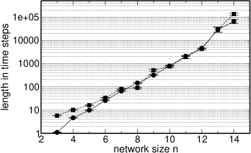
Figure 2: Limit cycle dynamics of a minimal network of $2$ vertices. b) Length of transients and limit cycles in networks of type II.

Networks of type II have much longer limit cycles and transients. Because of numerical limitations we were only able to determine cycle lengths for small networks. As shown in figure 2b) the typical transient and cycle lengths both grow approximately exponentially.

3.2 Vertex degrees and internal states

To characterize the networks resulting from the two different evolution laws, we measured several key quantities, including the distribution of node degrees (also called the vertex degree sequence), the distribution of node states $x_{i}$, the distribution of bond states $J_{ij}$, as well as temporal and spatial fluctuations of these quantities. The vertex degree distribution in dependence on $\lambda_{1}$ for a network of $200$ vertices is shown in figure 3a) and b) for network law I and II respectively. The second parameter was fixed as $\lambda_{2}=1.2\cdot\lambda_{1}$ to implement a reasonable hysteresis in the dynamical addition and removal of edges and the degrees were observed after a transient of $10$ time steps, i.e., prevalently still in a transient dynamics regime. The network structure undergoes a series of changes for increasing $\lambda_{1/2}$.

Networks of type I evolve from almost fully connected simplex networks to more sparse connectivities with increasing $\lambda_{1/2}$. There is a regime, where few vertices with very high degree coexist with many vertices with a low degree (around $\lambda_{1}=60$), which is reminiscent of the situation in small world networks. We, however, observe a bimodal distribution (with very sharp peaks in each given network, see figure 3) rather than a power law of abundance of node degrees. For large $\lambda_{1/2}$ the network eventually breaks apart and all nodes have vertex degree $0$.

For networks of type II the situation is – as expected – inverse with respect to $\lambda_{1/2}$. The networks are trivial with vertex degree $0$ for all nodes for small $\lambda_{1/2}$ and connect increasingly dense for increasing $\lambda_{1/2}$. In this family of networks, the distribution of vertex degrees is always fairly broad and remains such up to large $\lambda_{1/2}$. We observe an intriguing structure of multiple maxima of the distributions in a wide range of $\lambda_{1/2}$ values.

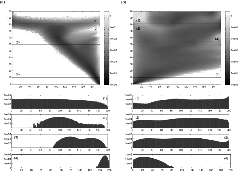
Figure 3: Distribution of abundance of node degrees in dependence on $\lambda_{1}$ (a: network type I, b: network type II). The second parameter was fixed to $\lambda_{2}=1.2\cdot\lambda_{1}$, $n=200$, and the total abundances shown are collected over 10990 different initial conditions. I.e., for each $\lambda_{1}$ ($y$ axis) the colors of the pixels show the number of times the node degree (corresponding to the $x$ position) appeared in the set of graphs generated with 10990 initial conditions. Note the logarithmic scale on the color scale and the y axes of the examples.

The observed structure of groups of highly connected and less connected vertices in the averaged distributions may arise from each given network realization having these two groups of vertices or appear due to the existence of two different types of networks. To probe these possibilities, we examined the abundance distribution of node degrees for individual initial conditions (Fig. 4). In all examples we observe the same structure as in the averaged picture (Fig. 3a), such that we have to conclude that there is only one type of network for a given $\lambda_{1},\lambda_{2}$ pair that has a structured vertex degree distribution. Furthermore, careful examination shows that this distribution can – unlike in the averaged picture – be fairly sharp, with often only one or two prevalent values for the vertex degree. The same is true for networks of type II: Distributions resemble the averaged picture but often with sharp peaks for a single value for the vertex degree (data not shown).

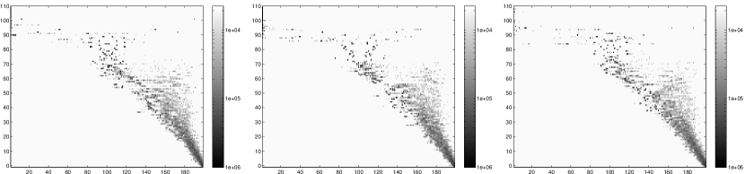
Figure 4: Distribution of abundance of node degrees in network I for three separate examples of initial conditions, dependent on $\lambda_{1}$ (again $\lambda_{2}=1.2\cdot\lambda_{1}$ and $n=200$). Note again the logarithmic color scale. All examples reflect the overall structure of the averaged data, thus showing that the appearance of hubs with large vertex degree and vertices with small degree actually occurs within the same network and at the same time and is not an artifact of averaging over many initial conditions

The temporal fluctuations, $\text{deg}_{i}(t+1)-\text{deg}_{i}(t)$, of vertex degrees give us insight into the stability of the network structure. For network law I we observe at $\lambda_{1}\approx 35$ an abrupt phase-transition from basically no temporal fluctuations in the node degrees (“frozen network”) to fairly high fluctuations (“liquid network”). For even larger $\lambda$, the fluctuations slowly abate in agreement with the smaller overall vertex degrees. It is surprising that the transition is so abrupt especially in the face of the much smoother development of the distribution of vertex degrees (Fig. 3).

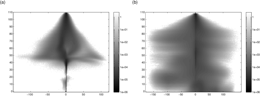
Figure 5: Distribution of abundance of temporal changes in node degrees dependent on $\lambda_{1}$ (again $\lambda_{2}=1.2\cdot\lambda_{1}$ and $n=200$). Note again the logarithmic color scale.

While the node degrees instruct us on the geometry of the CA graph, i.e., presumably on the structure of space, the state variables $s_{i}$ tell us something about an “energy” or “mass” density in some appropriate sense. As explained above the sum over local states, $\sum_{I}s_{i}$, is conserved, and hence is the sum of changes $\sum_{I}\Delta s_{i}=0$. This does, however, not imply that the distribution of $s_{i}$ or changes in $s_{i}$ are trivial. Figure 6 shows the maps for different node value distributions depending on $\lambda_{1}\in\{1,\ldots,111\}$ and $\lambda_{2}=1.2\lambda_{1}$.

The results are, as expected, very different for the two network types. Networks of type I have a clear region of intermediate $\lambda$ values where the distribution of node states is strongly bimodal for $62\leq\lambda_{1}\leq 85$. For smaller $\lambda$, i.e., for less bonds being switched off, there is a broad distribution of node states, and for larger $\lambda$ values, we observe a sharp unimodal distribution around $0$ corresponding to disconnected graphs, in which the node states are basically frozen in their initial values. Intriguingly, the transitions between the different types of state distributions occur at sharp values of $\lambda$ reminiscent of phase transitions.

Networks of type II have no bimodal distributions of node values, but there is a visible modulation in the width of node state distributions with different values of $\lambda_{1}$. For some $\lambda$ values, the distribution of observed states is rather sharp, for others rather wide. It is also interesting to note that, contrary to the naive expectation, the total width of the distributions is slightly larger than for networks of type I (note the light blue left and right tails for $\lambda_{1}\sim 60$). The fact that nodes with similar node state are connected and can reach some equilibrium and nodes with very different states are separate and can not interact (equilibrate) directly seems to allow such “outlier” states.

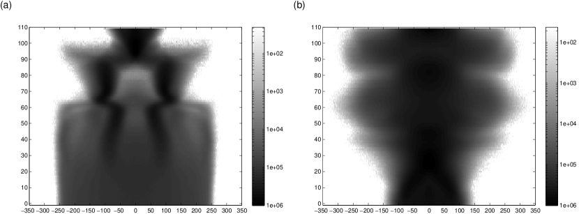
Figure 6: Distribution of abundance of node states in dependence on $\lambda_{1}$ (again $\lambda_{2}=1.2\cdot\lambda_{1}$ and $n=200$). As before, each line corresponds to a fixed pair of $\lambda_{1},\lambda_{2}$ and shows a distribution of observed node states in a logarithmic color code. Dark red pixels correspond to node states that are observed very often, and dark blue are states that are never observed.

4 Dimensionality

When studying such models as described above, it is of tantamount importance to find certain effective geometric characteristics of the large scale behavior of such irregular (in the small) networks. This holds the more so if one plans to perform some coarse-graining or continuum limit. It is evident that, in particular in the latter situation, only global features can be significant while, on the other hand, the finer details on small scales should be ignored.

The notion of dimension is one of these fundamental organizing concepts. There exist of course quite a few different versions of this concept in the mathematical literature, most of which, while looking useful at first glance, have to be dismissed on second thoughts. We will not give the pros and cons of all the different notions (a more detailed discussion can e.g. be found in [22] and [25]), let us only make the following point clear. The discrete models we are dealing with are not to be understood as some sort of tessellation of a preexisting continuous background manifold like in algebraic topology. In that case it would for example be reasonable to use the dimensional concept employed in simplicial complexes.

In our case, exactly the opposite is true. We view the continuum as an emergent limit structure, being the result of a (complicated) renormalisation group like process of coarse-graining. In this process, due to the rescaling of geometric scales, more and more vertices and links are absorbed in the infinitesimal neighborhoods of the emerging points of the continuum. As a consequence, what amounts to a local definition of dimension in the continuum is actually a large scale concept on the network, involving practically infinitely many vertices and their wiring.

Halpern and Ilachinski make a certain suggestion in their work (see e.g. [23]), which also happens to be a distinctly local concept. They define the effective dimensionality as the ratio of the number of next-nearest neighbors to the number of nearest neighbors averaged over the set of sites of the network. It is a typical property of most of the different dimensional concepts that they usually coincide on very regular spaces. This is for example well-known for the various notions of fractal dimension (cf. e.g. [28] or [29]). For the notion introduced above we have for instance in the case of $\mathbb{Z}^{2}$: $N_{nn}(x)=8,N_{n}(x)=4$, i.e. $D_{IH}=2$ and correspondingly for higher dimensions. However, for other lattices which are not so regular or translation invariant, i.e. having a more complicated local neighborhood structure, this is no longer true. While one would still like to associate on physical grounds in many cases their dimension with the corresponding embedding dimension of the ambient space, the above quotient may yield a different value.

The deeper reason is that the accidental near-order of the lattice may differ from its more important far-order. This phenomenon and the following physical argument motivated us to choose a different notion of intrinsic dimension which has a lot of very nice and desirable properties as has been shown in the papers we cited above. Originally we were primarily motivated by the following reasoning. What kind of intrinsic global property (i.e. being independent of some embedding dimension or accidental near-order) is relevant for the occurrence of phase transitions, critical behavior and the like? We wound up with the following answer: It is the increase of number of new agents or degrees of freedom one sees when one starts from a given lattice site and moves outward. This led to the following definition ( note that we introduce two slightly different notions which again coincide in many cases).

Definition 4.1

The (upper,lower) internal scaling dimension with respect to the vertex $x$ is given by

$$\overline{D}_{s}(x):=\limsup_{r\to\infty}(\ln\beta(x,r)/\ln r)\;,\,\underline{D}_{s}(x):=\liminf_{r\to\infty}(\ln\beta(x,r)/\ln r)$$ (14)

The (upper,lower) connectivity dimension is defined correspondingly as

$$\overline{D}_{c}(x):=\limsup_{k\to\infty}(\ln\partial\beta(x,k)/\ln k)+1\;,\,\underline{D}_{k}(x):=\liminf_{k\to\infty}(\ln\beta(x,k)/\ln k)+1$$ (15)

If upper and lower limit coincide, we call it the internal scaling dimension, the connectivity dimension, respectively.

In [25] we exhibited the close connection of this concept with important properties in various fields of pure mathematics (growth properties of metric spaces). Furthermore, when performing some continuum limit we could show that our notion of dimension makes contact with the various notions of fractal or Haussdorff-dimension.

5 Discussion

In the preceding sections we introduced and studied networks which are in various respects generalisations of structural dynamic CA, i.e., networks with both the site states and the wiring (link-distribution) being dynamic and (clock) time dependent. We thus realize an entangled dynamics of geometry and matter degrees of freedom as in, say, general relativity or quantum gravity. In contrast to more ordinary CA we admit a very high degree of disorder in the small while we hope that our network models find an attracting set in phase space after some transient time, thus displaying some patterns of global order. We are particularly interested in ordering phenomena on the geometric side. That is, we look for collective geometric properties like, e.g., dimension, which suggest that, after some coarse graining and/or rescaling, our networks display global smoothness properties which may indicate the transition into a continuum-like macro state.

We underpin our investigation by a quite detailed quantitative computational analysis of various (large scale) characteristics of our model networks as, e.g., vertex degree distribution, fluctuation patterns in site and/or link states, etc. There are indications that for certain choices of the parameters, labelling our model networks, we witness something akin to structural phase transitions.

It is particularly noteworthy that one of our model networks (after a very short transient time) enters a periodic state of period only six, and this being practically independent of the chosen initial state. Given the huge possible local fluctuations in both site states and link distribution the extremely short period is remarkable. This phenomenon has also been observed in other kinds of networks but nevertheless remains somewhat mysterious.

References

- [1] A.Ilachinski: “Cellular Automata, a Discrete Universe”, World Scient. Publ., Singapore 2001
- [2] K.Zuse:“The Computing Universe”, Int.J.Theor.Phys. 21(1982)589
- [3] R.P.Feynman: “Simulating Physics with Computers”, Int.J.Theor.Phys. 21(1982)467
- [4] E.Fredkin: ”Digital Mechanics”, Physica D45(1990)254 or the (programmatic) material on his homepage http://www.digitalphilosophy.org
- [5] D.Finkelstein: “The Space-Time Code”, Phys.Rev. 184(1969)1261
- [6] G.’t Hooft: “Quantization of Discrete Deterministic Theories”, Nucl.Phys. B 342(1990)471
- [7] G.’t Hooft: “Quantum Gravity as a Dissipative Deterministic System”, Class.Quant.Grav. 16(1999)3263, gr-qc/9903084
- [8] S.Wolfram: ”A New Kind of Science”, Wolfram Media 2002
- [9] K.Svozil: ”Computational Universe”, Chaos,Solitons,Fractals 25(2005)845 or physics/0305048
- [10] G.’t Hooft: ”Can Quantum Mechanics Be Reconciled With CA?”, Int.J.Theor.Phys. 42(2003)349
- [11] K.Svozil: “Are Quantum Fields Cellular Automata?”, Phys.Lett. 119A(1987)153
- [12] M.Requardt: “Scale Free Small-World Networks and the Structure of Quantum Space-Time”, gr-qc/0308089
- [13] A.Lochmann,M.Requardt: “An Analysis of the Transition Zone Between the various Scaling Regimes in the Small-World Model”, J.Stat.Phys. 122(2006)255 or cond-mat/0409710
- [14] M.Requardt: ”A Geometric Renormalisation Group and Fixed-Point Behavior in Discrete Quantum Space-Time”, J.Math.Phys. 44(2003)5588 or gr-qc/0110077
- [15] S.Kauffmann: “Origins of Order: Self-Organisation and Selection in Evolution”, Oxford Univ.Pr., Oxford 1993
- [16] S.Kauffmann: “At Home in the Universe, The Search for Laws of Self-Organisation and Complexity”, Oxford Univ.Pr., Oxford 1995
- [17] S.Kauffmann: “Antichaos and Adaption”, Sci.Am. 265(1991)76
- [18] C.G.Langton: ed. “Artificial Life: Proc. of an Interdisciplinary Workshop on the Synthesis and Simulation of Living Systems, Sept. 1987, Los Alamos, Addison-Wesley Publ. N.Y. 1989
- [19] M.Gardner: “On CA, Self-Reproduction. The Garden of Eden and the Game of Life”, Sci.Am. 224(1971)112
- [20] M.Requardt: ”Cellular Networks as Models for Planck-Scale Physics”, J.Phys. A:Math.Gen. 31(1998)7997 or hep-th/9806135
- [21] T.Nowotny,M.Requardt: ”Pregeometric Concepts on Graphs and Cellular Networks”, Chaos,Solitons and Fractals 10(1999)469 (invited paper) or hep-th/9801199
- [22] T.Nowotny,M.Requardt: ”Dimension Theory on Graphs and Networks”, J.Phys. A:Math.Gen. 31(1998)2447 or hep-th/9707082
- [23] P.Halpern: ”Sticks and Stones: A Guide to SDCA”, Am.J.Phys. 57(1989)405
- [24] R.Alonso-Sanz: “Reversible Structurally CA with Memory”, preprint 2006, submitted to J.Cell.Aut.
- [25] M.Requardt: ”The Continuum Limit of Discrete Geometries”, Int.J.Geom.Meth.Mod.Phys. 3(2006)285 or math-ph/0507017
- [26] T.Toffoli, N.Margolus: “Cellular Automaton Machines”, MIT Pr., Cambridge Mass. 1987
- [27] R. Huerta and M. Rabinovich, “Reproducible Sequence Generation In Random Neural Ensembles”, Phys Rev Lett 93: 238104 (2004)
- [28] G.A.Edgar: “Measure, Topology and Fractal Geometry”, Springer, N.Y. 1990
- [29] K.J.Falconer: “Fractal Geometry”, Wiley, Chichester 1990
- [30]