Band-Insulator-Metal-Mott-Insulator transition in the
half–filled $t-t^{\prime}$ ionic-Hubbard chain

Abstract

We investigate the ground state phase diagram of the half-filled $t-t^{\prime}$ repulsive Hubbard model in the presence of a staggered ionic potential $\Delta$, using the continuum-limit bosonization approach. We find, that with increasing on-site-repulsion $U$, depending on the value of the next-nearest-hopping amplitude $t^{\prime}$, the model shows three different versions of the ground state phase diagram. For $t^{\prime}<t^{\prime}_{\ast}$, the ground state phase diagram consists of the following three insulating phases: Band-Insulator at $U<U_{c}$, Ferroelectric Insulator at $U_{c}<U<U_{s}$ and correlated (Mott) Insulator at $U>U_{c}$. For $t^{\prime}>t^{\prime}_{c}$ there is only one transition from a spin gapped metallic phase at $U<U_{c}$ to a ferroelectric insulator at $U>U_{c}$. Finally, for intermediate values of the next-nearest-hopping amplitude $t^{\prime}_{\ast}<t^{\prime}<t^{\prime}_{c}$ we find that with increasing on-site repulsion, at $U_{c1}$ the model undergoes a second-order commensurate-incommensurate type transition from a band insulator into a metallic state and at larger $U_{c2}$ there is a Kosterlitz-Thouless type transition from a metal into a ferroelectric insulator.

I Introduction

During the last decades, the Mott metal-insulator transition has been a subject of great interest.Mott_Book_90 ; Gebhard_Book_97 ; IFT_98 In the canonical model for this transition – the single-band Hubbard model – the origin of the insulating behavior is the on-site Coulomb repulsion between electrons. For an average density of one electron per site, the transition from the metallic to the insulating phase is expected to occur with increasing on-site repulsion when the electron-electron interaction strength $U$ exceeds a critical value $U_{c}$, which is usually of the order of the delocalization energy. Although the underlying mechanism driving the Mott transition is by now well understood, many questions remain open, especially about the region close to the transition point where perturbative approaches fail to provide reliable answers.

The situation is more fortunate in one dimension, where non-perturbative analytical methods together with well-controlled numerical approaches allow to obtain an almost complete description of the Hubbard model and its dynamical properties.EFGKK_2005 However, even in one dimension, apart from the exactly solvable cases, a full treatment of the fundamental issues related to the Mott transition still constitutes a hard and challenging problem.

Intensive recent activity is focused on studies of the extended versions of the Hubbard model which display, with increasing Coulomb repulsion, a transition from a band-insulator (BI) into the correlated (Mott) insulator phase. Various models considered include those, which show a continuous evolution from a BI into the MI phaseRosch_06 ; Anfuzo_Rosch_06 ; Monien_06 as well as those, where the transformation of a BI to a correlated (Mott) insulator takes place via a sequence of quantum phase transitions.Fab_99 ; Brune_03 ; Man_04 ; Otsu_05 ; TAJN_06 ; Randeria_06 ; LHJ_06 ; Dagotto_06

Intensive recent activity is focused on studies of the extended versions of the Hubbard model with alternating on-site energies $\pm\Delta$, known as the ionic Hubbard model (IHM). Fab_99 ; Brune_03 ; Man_04 ; Otsu_05 ; TAJN_06 ; Randeria_06 ; LHJ_06 ; Dagotto_06 ; Tor_01 ; Aligia_04 ; Aligia_Hallberg_05 ; Batista_Aligia_05 ; Scalettar_06 The model has a long-term history,Hub_Torr_81 however the increased current interest widely comes from the possibility to describe the interaction driven BI to MI transition within one model. In one dimension this evolution with increasing on-site repulsion is characterized by two quantum phase transitions: first a (charge) transition from the BI to a ferroelectric insulator (FI) and second, with further increased repulsion, a (spin) transition from the FI to a correlated MI.Fab_99 Detailed numerical studies of the 1D IHM clearly show, that an unconventional metallic phase is realized in the ground state of the model only at the charge transition point and the BI and MI phases are separated in the phase diagram by the insulating ferroelectric phase.Brune_03 ; Man_04 ; Otsu_05 ; TAJN_06 Studies of the 2D IHM using the cluster dynamical mean field theory, reveal a similar phase diagram.Dagotto_06

On the other hand, recent studies of the IHM using the dynamical mean field theory (DMFT) approach, show that in high dimensions the BI phase can be separated from the MI phase by the finite stripe of a metallic phase.Randeria_06 Moreover, recent studies of the IHM with site diagonal disorder using the DMFT approach, also show the existence of a metallic phase which separates the BI phase from the MI phase in the ground state phase diagram of the disordered IHM.LHJ_06 It looks so, that in low-dimensional models with perfect nesting of the Fermi surface, the metallic phase is reduced to the charge transition line, while in higher dimensions the space for realization of a metallic phase opens. Note that the very presence of a metallic phase along critical lines separating two insulating phases is common for 1D systems with competing short-range interactions responsible for the dynamical generation of a charge gap.Emery_79 However, one-dimensional models of correlated electrons, showing with increasing electron-electron coupling a transition from an insulating to a metallic phase are less known.Note_1

In this paper we show, that the one-dimensional half-filled ionic-Hubbard model supplemented with the next-nearest-neighbor hopping term ($t^{\prime}$) is possibly the simplest one-dimensional model of correlated-electrons, which shows a ferroelectric ground state in a wide area of the phase diagram easily controlled by the model parameters.

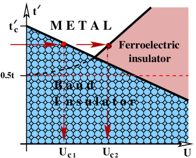
We also show that in a certain range of the model parameters the $t-t^{\prime}$ ionic-Hubbard chain shows, with increasing Coulomb repulsion, a transition from a band-insulator to a metal and, with further increase of the Hubbard repulsion, a transition from a metal to a ferroelectric insulator (see Fig.1).

Figure 1: Qualitative phase diagram of the half-filled $t-t^{\prime}$ ionic-Hubbard chain for $t^{\prime}>0.5t$ and weak and moderate values of the on-site Hubbard repulsion $U$. The parameter $t^{\prime}_{c}=0.5t\sqrt{1+(\Delta/4t)^{2}}+\Delta/8$ corresponds to the insulator to metal transition point in the free ionic chain, where $\Delta/2$ is the amplitude of alternating ionic potential. The dashed curve line marks the I-M transition line in the $t-t^{\prime}$ Hubbard model, corresponding to the case $\Delta=0$. The dashed line $t^{\prime}=0.5t$ is given as an eye guide.

The paper is organized as follows. In Section II, the model and its several important limiting cases are briefly reviewed. In the Section III the weak-coupling bosonization description is obtained. The results are summarized in Section IV.

II The model

The Hamiltonian we consider is given by

$${\cal H} = -t\,\sum_{n,\sigma}\left(c^{\dagger}_{n,\sigma}c^{\phantom{\dagger}}_{n+1,\sigma}\,+\,c^{\dagger}_{n+1,\sigma}c^{\phantom{\dagger}}_{n,\sigma}\right)$$ (1)

$$+ t^{\prime}\,\sum_{n,\sigma}\left(c^{\dagger}_{n,\sigma}c^{\phantom{\dagger}}_{n+2,\sigma}+c^{\dagger}_{n+2,\sigma}c^{\phantom{\dagger}}_{n,\sigma}\right)$$

$$+\sum_{n,\sigma}\left(\delta\mu+(-1)^{n}\frac{\Delta}{2}\right)\rho_{n,\sigma}\,+U\,\sum_{n}\,\rho_{n,\uparrow}\rho_{n,\downarrow}\,.$$

Here $c^{\dagger}_{n,\sigma}$ $(c^{\phantom{\dagger}}_{n,\sigma})$ are electron creation (annihilation) operators on site $n$ and, with spin projection $\sigma=\uparrow,\downarrow$, $\rho_{n,\sigma}=c^{\dagger}_{n,\sigma}c^{\phantom{\dagger}}_{n,\sigma}$. The nearest-neighbor hopping amplitude is denoted by $t$, the next-nearest-neighbor hopping amplitude by $t^{\prime}$ ($t,t^{\prime}>0$), $\Delta$ is the potential energy difference between neighboring sites, $U$ is the on-site Coulomb repulsion and the band-filling is controlled by the proper shift of the chemical potential $\delta\mu$. For $t^{\prime}=0$, we recover the Hamiltonian of the ordinary ionic-Hubbard chain, while for $\Delta=0$ the Hamiltonian of the $t-t^{\prime}$ Hubbard chain.

At $U=0$ the model is easily diagonalized in momentum space to give a dispersion relation in the first Brillouin zone $-\pi/2<k<\pi/2$

$$E_{\pm}(k)=2t^{\prime}\cos 2k-\delta\mu\pm\sqrt{4t^{2}\cos^{2}k+(\Delta/2)^{2}}\,.$$ (2)

Let us first analyze the dispersion relation (2). For $t,t^{\prime}>0$ the absolute maximum of the upper band is reached at $k=0$, while the absolute minimum

$$E^{+}_{min}=-2t^{\prime}-\delta\mu+\Delta/2\,,$$ (3)

at $k=\pm\pi/2$.

The lower band shows a more complicated dependence on the model parameters. For

$$t^{\prime}\,<\,t^{\prime}_{\ast}\,=\,0.5t~{}\sqrt{1+(\Delta/4t)^{2}}-\Delta/8$$ (4)

the absolute minimum of the lower band is reached at $k=0$ and while the absolute maximum at $k=\pm\pi/2$ and is equal to

$$E^{-}_{max}=-2t^{\prime}-\delta\mu-\Delta/2\,.$$ (5)

In the case of half-filling the lower band is completely filled and the upper band is empty. The system is a band-insulator with a gap in the excitation spectrum

$$\Delta_{exc}\equiv E^{+}_{min}-E^{-}_{max}=\Delta.$$ (6)

The corresponding shift of the chemical potential $\delta\mu=-2t^{\prime}$ is easily determined from the condition $E^{+}_{min}+E^{-}_{max}=0$. Thus, for $t^{\prime}<t^{\prime}_{\ast}$ the ground state and low-energy excitation spectrum of the model are not affected by the increase of the next-nearest hopping amplitude $t^{\prime}$.

The effect of $t^{\prime}$ becomes nontrivial for $t^{\prime}\,>\,t^{\prime}_{\ast}$, when the absolute maximum of the lower band

$$E^{-}_{max}=2t^{\prime}-\delta\mu-\sqrt{4t^{2}+(\Delta/2)^{2}}\,$$

is reached at $k=0$. For

$$t^{\prime}\,<\,t^{\prime}_{c}\equiv\,0.5t~{}\sqrt{1+(\Delta/4t)^{2}}+\Delta/8$$ (7)

the absolute maximum of the lower band at $k=0$ remains lower than the absolute minimum of the upper band at $k=\pi/2$. Therefore the system remains an insulator, but the indirect gap

$$\Delta_{B}=\frac{\Delta}{2}\,+\,\sqrt{4t^{2}+(\Delta/2)^{2}}-4t^{\prime}$$ (8)

decays linearly with increasing $t^{\prime}$ and finally vanishes at $t^{\prime}=t^{\prime}_{c}$. It is straightforward to find, that the corresponding shift of the chemical potential which ensures half-filling in this case is given by $\delta\mu=-2t^{\prime}_{\ast}$.

At $t^{\prime}=t^{\prime}_{c}$ the $t-t^{\prime}$ ionic chain experiences a transition from a band-insulator to a metal. For $t^{\prime}>t^{\prime}_{c}$ a gapless phase is realized, corresponding to a metallic state with four Fermi points $\pm k_{F1}$ and $\pm k_{F2}$, which satisfy the relation $2(k_{F1}-k_{F2})=\pi$.

At $U>0$ several limiting cases of the model (1) have been the subject of intensive current studies. In particular intensive recent activity has been focused on studies of the ground state phase diagram of the ionic-Hubbard model (IHM), corresponding to the limiting case $t^{\prime}=0$ and of the $t-t^{\prime}$ Hubbard model corresponding to the limiting case $\Delta=0$.

Current interest in this model mostly originates from the possibility to describe the evolution from the band insulator (BI) at $U\ll\Delta$ into a correlated (Mott) insulator (MI) for $U\gg\Delta$ within a single system. Fab_99 ; Tor_01 ; Brune_03 ; Man_04 ; Aligia_04 ; Aligia_Hallberg_05 ; Batista_Aligia_05 ; Otsu_05 ; TAJN_06 ; Randeria_06 ; LHJ_06 ; Dagotto_06 In the case of the one-dimensional ionic-Hubbard model this evolution is characterized by two quantum phase transitions in the ground state. Fab_99 With increasing $U$ the first is a charge transition at $U=U_{c}$, from the BI to a bond-ordered, spontaneously dimerized, ferroelectric insulator (FI). At the transition point the charge sector of the model becomes gapless, however for $U>U_{c}$ the charge gap opens again. When $U$ is further increased, the second (spin) transition from the FI phase into the MI phase takes place at $U_{s}>U_{c}$. At this transition the spin gap vanishes and the spin sector remains gapless in the MI phase for $U>U_{s}$. A similar ground state phase diagram has been recently established also in the case of 2D IHM using the cluster dynamical mean field theory.Dagotto_06 Thus, for low-dimensional versions of the IHM with perfect nesting property of the Fermi surface, the transition from a BI to a FI is characterized by the presence of a metallic (charge gapless) phase only at the transition line. In the ground state phase diagram of the BI phase is separated from the MI phase by a FI phase.Fab_99 ; Man_04 ; TAJN_06 ; Dagotto_06

The homogeneous half-filled $t-t^{\prime}$ Hubbard chain is a prototype model to study the metal-insulator transition in one dimension and therefore has been the subject of intensive studies in recent years. Fabrizio_96 ; Kuroki_97 ; Fabrizio_98 ; DaulNoack_98 ; DaulNoack_00 ; AebBaerNoack_01 ; Gros_01 ; Gros_02 ; Torio_03 ; Gros_04 ; Fabrizio_04 ; JNB_06 As in the case of the ionic-chain, in the $t-t^{\prime}$ Hubbard model an increase of the next-nearest hopping $t^{\prime}$ changes the topology of the Fermi surface: at half-filling and for $t^{\prime}<0.5t$, the electron band of has two Fermi points at $k_{F}=\pm\pi/2$, separated from each other by the umklapp vector $q=\pi$. In this case, a weak-coupling renormalization group analysis predicts the same behavior as for $t^{\prime}=0$ - the dynamical generation of a charge gap for $U>0$, and gapless magnetic excitations.Fabrizio_96

For $t^{\prime}>0.5t$, the Fermi level intersects the one-electron band at four points $\left(k_{F}^{\pm}\neq\pm\pi/2\right)$. For weak Hubbard coupling ($U\ll t$) the infrared behavior is governed by the low-energy excitations in the vicinity of the four Fermi points, in full analogy with the two-leg Hubbard model. BalentsFisher_96 The Fermi vectors $k_{F}^{\pm}$ are sufficiently far from $\pi/2$ to suppress first-order umklapp processes and therefore the charge excitations are gapless, however the spin degrees of freedom are becoming gapped.BalentsFisher_96 ; Fabrizio_96 ; DaulNoack_00 ; Gros_01 ; Torio_03 Since at half-filling $4(k_{F}^{+}-k_{F}^{-})=2\pi$, with increasing on-site repulsion higher-order umklapp processes become relevant for intermediate values of $U$. Therefore, starting from a metallic region for small $U$ at a given value of $t^{\prime}$ ($t^{\prime}>0.5t$), one reaches a transition line $U=U_{c}(t^{\prime})$ above which the system is insulating with both charge and spin gaps. Fabrizio_96

As we will show in this paper for $t^{\prime}<t^{\prime}_{\ast}$, where the topology of Fermi surface is restricted to two Fermi points, the ground state phase diagram of the $t-t^{\prime}$ ionic-Hubbard chain coincides with that of the IHM, while for $t^{\prime}>t^{\prime}_{c}$, where the model is characterized by four Fermi points - it coincides with that of the $t-t^{\prime}$ Hubbard chain. Most interesting is the case $t^{\prime}_{\ast}<t^{\prime}<t^{\prime}_{c}$, where with increasing on-site repulsion we observe two transitions in the ground state: at $U_{c1}$ the model undergoes a second-order commensurate-incommensurate type transition from a band insulator into a metallic state and at large $U_{c2}$ there is a Kosterlitz-Thouless type transition from a metal into a correlated ferroelectric insulator.

III Bosonization results

In this section we analyze the low-energy properties of the $t-t^{\prime}$ ionic-Hubbard chain using the continuum-limit bosonization approach. We first consider the regime $U,\Delta,t^{\prime}\ll t$, linearize the spectrum in the vicinity of the two Fermi points $k_{F}=\pm\pi/2$ and go to the continuum limit by substituting

$$c_{n\sigma}\rightarrow\sqrt{a_{0}}\,\Big{[}i^{n}\psi_{R\sigma}(x)+(-i)^{n}\psi_{L\sigma}(x)\,\Big{]}\,,$$ (9)

where $x=na_{0}$, $a_{0}$ is the lattice spacing, and $\psi_{R\sigma}(x)$ and $\psi_{L\sigma}(x)$ describe right-moving and left-moving particles, respectively. The chosen type of decoupling of the model into ”free” and ”interaction” parts allows to treat the gap ”creating” ($\Delta$ and $U$) and gap ”destructing” ($t^{\prime}$) terms on equal footing and reveals easily their competition within the continuum-limit treatment.

The right and left fermionic fields are bosonized in the standard way:GNT

$$\psi_{R\sigma}(x) = \frac{1}{\sqrt{2\pi a_{0}}}e^{{\it i}\sqrt{\pi}[\Phi_{\sigma}(x)+\Theta_{\sigma}(x)]},$$ (10)

$$\psi_{L\sigma}(x) = \frac{1}{\sqrt{2\pi a_{0}}}e^{-{\it i}\sqrt{\pi}[\Phi_{\sigma}(x)-\Theta_{\sigma}(x)]}\,,$$ (11)

where $\Phi_{\sigma}(x)$ and $\Theta_{\sigma}(x)$ are dual bosonic fields, $\partial_{t}\Phi_{\sigma}=v_{F}\partial_{x}\Theta_{\sigma}$ and $v_{F}=2ta_{0}$.

This gives the following bosonized Hamiltonian:

$${\cal H}={\cal H}_{\uparrow}+{\cal H}_{\downarrow}+{\cal H}_{\uparrow\downarrow}\,,$$

where

$${\cal H}_{\sigma} = \int dx\Big{\{}\frac{v_{F}}{2}\big{[}\left(\partial_{x}\Phi_{\sigma}\right)^{2}+\left(\partial_{x}\Theta_{\sigma}\right)^{2}\big{]}$$ (12)

$$-\frac{\mu_{eff}}{\sqrt{\pi}}\partial_{x}\Phi_{\sigma}-\frac{\Delta}{2\pi a_{0}}\sin\sqrt{4\pi}\Phi_{\sigma}\,\Big{\}}\,\quad\left(\sigma=\uparrow,\downarrow\right)$$

and

$${\cal H}_{\uparrow\downarrow} = \int dx\Big{\{}\,\big{[}\,\frac{U}{\pi}\partial_{x}\Phi_{\uparrow}\partial_{x}\Phi_{\downarrow}$$ (13)

$$+\frac{U}{\pi^{2}a_{0}^{2}}\sin\sqrt{4\pi}\Phi_{\uparrow}\sin\sqrt{4\pi}\Phi_{\downarrow}\,\big{]}\Big{\}}.$$

Here we have introduced

$$\mu_{{\it eff}}=2t^{\prime}+\delta\mu$$

$$=\left\{\begin{array}[]{l}\hskip 17.07182pt0\hskip 36.98866pt\mbox{for}\hskip 14.22636ptt^{\prime}<t^{\prime}_{\ast}\\ 2\left(t^{\prime}-t^{\prime}_{\ast}\right)\hskip 17.07182pt\mbox{for}\quad\hskip 2.84544ptt^{\prime}_{\ast}<t^{\prime}<t^{\prime}_{c}\\ \end{array}\right.\,.$$ (16)

The next step is to introduce the charge

$$\varphi_{c}={\textstyle\frac{1}{\sqrt{2}}}(\phi_{\uparrow}+\phi_{\downarrow}),\qquad\vartheta_{c}={\textstyle\frac{1}{\sqrt{2}}}(\theta_{\uparrow}-\theta_{\downarrow})$$ (17)

and spin fields

$$\varphi_{s}={\textstyle\frac{1}{\sqrt{2}}}(\varphi_{\uparrow}-\varphi_{\downarrow}),\qquad\vartheta_{s}={\textstyle\frac{1}{\sqrt{2}}}(\theta_{\uparrow}-\theta_{\downarrow})$$ (18)

to describe corresponding degrees of freedom. After a simple rescaling, we arrive at the bosonized version of the Hamiltonian (1)

$${\cal H}={\cal H}_{s}+{\cal H}_{c}+H_{cs}\,,$$

where

$${\cal H}_{c} = \int dx\Big{\{}\frac{v_{c}}{2K_{c}}(\partial_{x}\varphi_{c})^{2}+\frac{v_{c}K_{c}}{2}(\partial_{x}\vartheta_{c})^{2}$$ (19)

$$-\mu_{\text{eff}}\sqrt{\frac{2}{\pi}}\partial_{x}\varphi_{c}-\frac{U}{2\pi^{2}a_{0}^{2}}\cos(\sqrt{8\pi}\varphi_{c})\Big{\}},$$

$${\cal H}_{s} = \int dx\Big{\{}\frac{v_{s}}{2}\big{[}(\partial_{x}\varphi_{s})^{2}+\frac{1}{2}(\partial_{x}\vartheta_{s})^{2}\big{]}$$ (20)

$$+\frac{U}{2\pi^{2}a_{0}^{2}}\cos(\sqrt{8\pi}\varphi_{s})\Big{\}},$$

$${\cal H}_{cs} = -\frac{\Delta}{\pi a_{0}}\int dx\,\sin\left(\sqrt{2\pi}\varphi_{c}\right)\cos\left(\sqrt{2\pi}\varphi_{s}\right)$$ (21)

with the charge stiffness parameter $K_{c}\simeq 1-U/4\pi t$ at $U/4\pi t\ll 1$.

III.1 Non-interacting case

To assess the accuracy of the continuum-limit treatment it is instructive to start our bosonization analysis from the exactly solvable case of the ionic-chain.

At $U=0$ the system is decoupled into the ”up” and ”down” spin component parts ${\cal H}={\cal H}_{\uparrow}+{\cal H}_{\downarrow}$, where for each spin component the Hamiltonian is the sine-Gordon model with topological term (12). Each of these Hamiltonians is the standard Hamiltonian for the commensurate-incommensurate transition, which has been intensively studied in the past using bosonization C_IC_transition and the Bethe ansatz.JNW_1984 This allows to apply the theory of commensurate-incommensurate transitions to the metal-insulator transition in the considered case of a half-filled $t-t^{\prime}$ chain with ionic distortion.

At $\mu_{eff}=0$, the model is described by the theory of two commuting sine-Gordon fields ($\sin\beta\Phi_{\sigma}$) with $\beta^{2}=4\pi$. In this case the excitation spectrum is gapped and the excitation gap is given by the mass of the ”up” (”down”) field soliton $M_{\uparrow}=M_{\downarrow}=\Delta/2$. In the ground state the $\Phi_{\uparrow}$ and $\Phi_{\downarrow}$ fields are pinned with vacuum expectation values $\langle 0|\Phi_{\sigma}|0\rangle=\sqrt{\pi}(n+1/4)$. Using the standard bosonized expression for the $2k_{F}$ modulated part of the charge density GNT

$$\rho_{c}(x) \simeq (-1)^{n}\frac{1}{\pi a_{0}}\sum_{\sigma}\sin(\sqrt{4\pi}\Phi_{\sigma}(x))$$ (22)

$$= \frac{(-1)^{n}}{2\pi a_{0}}\sin(\sqrt{2\pi}\varphi_{c}(x))\cos(\sqrt{2\pi}\varphi_{s}(x))$$

we obtain that at $\mu_{eff}=0$ the ground state of the system corresponds to a CDW type band-insulator with a single energy scale given by the ionic potential $\Delta$.

At $\mu_{eff}\neq 0$ it is necessary to consider the ground state of the sine-Gordon model in sectors with nonzero topological charge. The competition between the chemical potential term ($t^{\prime}$) and the commensurability energy given by $\Delta$ finally drives a continuous phase transition from a gapped (insulating) phase at $\mu_{{\it eff}}<\mu_{{\it eff}}^{c}$ to a gapless (metallic) phase at

$$\mu_{\text{eff}}>\mu_{\text{eff}}^{c}=\Delta/2\,.$$ (23)

Using (16) we easily obtain, that the critical value of the n-n-n hopping amplitude $t^{\prime}$, obtained from the condition (23) coincides with the exact value for the ionic-chain given in (7).

As we observe, the insulator-metal transition at $t^{\prime}>t^{\prime}_{c}$ is connected with a change of the topology of the Fermi surface and a corresponding redistribution of the electrons from the lower (”-”) band into the upper (”+”) band. We use as an order parameter of this transition the number $N_{+}$ of electrons transferred into the ”+” band, which is related to the value of the new Fermi point $k_{0}\sim\sqrt{\mu-\mu_{c}}$. At the transition point the compressibility of the system is

$$\partial E_{0}/\partial\mu\sim-k_{0}^{-1}=-(\mu-\mu_{c})^{-1/2}\,,$$ (24)

showing an inverse square-root singularity, where $E_{0}$ is the ground state energy.

Before we start to consider the interacting case, it is useful to continue our analysis of the noninteracting case, but within the basis of the charge and spin Bose fields, which is more convenient for interacting electrons.

The Hamiltonian we have to consider now is given by

$${\cal H} = \int dx\Big{\{}\frac{v_{F}}{2}\big{[}(\partial_{x}\varphi_{c})^{2}+(\partial_{x}\vartheta_{c})^{2}\big{]}-\mu_{\text{eff}}\sqrt{\frac{2}{\pi}}\partial_{x}\varphi_{c}$$ (25)

$$\hskip 28.45274pt+\frac{v_{F}}{2}\big{[}(\partial_{x}\varphi_{s})^{2}+\frac{1}{2}(\partial_{x}\vartheta_{s})^{2}\big{]}$$

$$\hskip 11.38109pt-\frac{\Delta}{\pi a_{0}}\sin\left(\sqrt{2\pi}\varphi_{c}\right)\cos\left(\sqrt{2\pi}\varphi_{s}\right)\Big{\}}\,.$$

We decouple the interaction term in a mean-field manner by introducing

$$m_{c} = \Delta\cdot\langle\cos\sqrt{2\pi}\varphi_{s}\rangle\,\,,$$ (26)

$$m_{s} = \Delta\cdot\langle\sin\sqrt{2\pi}\varphi_{c}\rangle\,,$$ (27)

and get the mean-field bosonized version of the Hamiltonian ${\cal H}={\cal H}_{c}+{\cal H}_{s}$ which is given by the two commuting quantum sine-Gordon models

$${\cal H}_{c} = \int dx\Big{\{}{v_{F}\over 2}[(\partial_{x}\vartheta_{c})^{2}+(\partial_{x}\varphi_{c})^{2}]$$ (28)

$$-\mu_{\text{eff}}\sqrt{\frac{2}{\pi}}\partial_{x}\varphi_{c}-\frac{m_{c}}{\pi a_{0}}\sin(\sqrt{2\pi}\varphi_{c})\Big{\}},$$

$${\cal H}_{s} = \int dx\Big{\{}{v_{F}\over 2}[(\partial_{x}\vartheta_{s})^{2}+(\partial_{x}\varphi_{s})^{2}]$$ (29)

$$-\frac{m_{s}}{\pi a_{0}}\cos(\sqrt{2\pi}\varphi_{s})\Big{\}}\,.$$

Although the mean-field Hamiltonian is once again given by the sum of two decoupled sine-Gordon models (see Eq. (12)), the dimensionality of the $\cos(\beta\phi)$ operators at $\beta^{2}=2\pi$ and $\beta^{2}=4\pi$ are different. Therefore, in marked contrast with the bosonized theory in terms of ”up” and ”down” fields (12), the pair of Hamiltonians given by (28)-(29) represents a very complex basis to describe the BI phase i.e. the CDW state with equal charge and spin gaps $\Delta_{c}=\Delta_{s}=\Delta/2$.

Nevertheless, below we use the benefit of the exact solution of the sine-Gordon model to get a qualitatively and almost quantitatively accurate description of the problem even in the ”spin-charge” basis. To see this, let us start from the case $\mu_{\text{eff}}=0$. We will use the following exact relations between the bare mass $m$ and the soliton physical mass $M$ for the sine-Gordon theory with $\beta^{2}=2\pi$Al_B_Zamolodchikov_95

$$M/\Lambda={\cal C}_{0}\left(m/\Lambda\right)^{2/3}\,,$$ (30)

and the exact expression for the expectation value of the $\cos\beta\phi$ fieldLuk_Zam_97

$$\langle\,\cos\sqrt{2\pi}\varphi\,\rangle={\cal C}_{1}\left(M/\Lambda\right)^{1/2}\,.$$ (31)

Here

$${\cal C}_{0}=\frac{2\Gamma\left(1/6\right)}{\sqrt{\pi}\Gamma\left(2/3\right)}\left[\frac{\Gamma(3/4)}{2\Gamma(1/4)}\right]^{\frac{2}{3}}$$ (32)

and

$${\cal C}_{1}=\frac{2}{3}\left(\frac{3\pi}{4}\right)^{1/4}\frac{\Gamma(3/4)}{\Gamma(1/4)}\,$$ (33)

and $\Lambda=2t$ is the bandwidth.

Using (30)-(33) one easily finds that

$$\Delta_{c}/\Lambda = {\cal C}_{0}\left(\Delta/\Lambda\right)^{2/3}\langle\,\cos\sqrt{2\pi}\varphi_{s}\,\rangle^{2/3}$$ (34)

$$= {\cal C}_{0}\,{\cal C}_{1}^{2/3}\left(\Delta/\Lambda\right)^{2/3}\left(M_{s}/\Lambda\right)^{1/3}\,$$

$$\Delta_{s}/\Lambda = {\cal C}_{0}\left(\Delta/\Lambda\right)^{2/3}\langle\,\sin\sqrt{2\pi}\varphi_{c}\,\rangle^{2/3}$$ (35)

$$= {\cal C}_{0}\,{\cal C}_{1}^{2/3}\left(\Delta/\Lambda\right)^{2/3}\left(M_{c}/\Lambda\right)^{1/3}\,.$$

The self-consistent solution of the Eqs. (34)-(35) gives

$$\Delta_{c}=\Delta_{s}=\gamma\Delta/2$$ (36)

with $\gamma=2{\cal C}^{3/2}_{0}{\cal C}_{1}=0.94256...$. Thus the mean-field treatment of the ionic-chain within the spin-charge basis gives not only a qualitatively correct but, rather quantitatively accurate description for the system in the BI phase.

For completeness of our description, let us now consider the insulator to metal transition in the ionic-chain in the charge-spin Bose field basis. The corresponding mean-field decoupled charge Hamiltonian is given by the $\beta^{2}=2\pi$ quantum sine-Gordon model with the topological term (28). From the exact solution of the SG modelDHN it is known that the excitation spectrum of the model at $\beta^{2}=2\pi$ consists of solitons and antisolitons with mass $M_{c}$, and soliton-antisoliton bound states (”breathers”) with masses $M_{c}^{n=1}=2M_{c}\sin(\pi/6)=M_{c}$ and $M_{c}^{n=2}=2M_{c}\sin(\pi/3)=\sqrt{3}M_{c}$. The transition from the BI into the metallic phase takes place when the effective chemical potential exceeds the mass of the lowest breather i.e. at $\mu_{eff}=M_{c}=\Delta/2$. For $\mu_{eff}>M_{c}$ the vacuum average of the charge field is not pinned at all, such that the spin gap $\langle M_{s}\rangle\sim\langle\sin(\sqrt{2\pi}\varphi_{c})\rangle=0$.

Thus, using the bosonization treatment we easily and with good numerical accuracy describe the exactly solvable case of the band-insulator to metal transition, which takes place in the $t-t^{\prime}$ ionic chain with increasing next-nearest-hopping amplitude $t^{\prime}$.

III.2 Interacting case

At $U\neq 0$ the use a similar mean-field decoupling allows us to rewrite the Hamiltonian as two commuting double sine-Gordon models ${\cal H}={\cal H}_{c}+{\cal H}_{s}$ where

$${\cal H}_{c} = \int dx\Big{\{}\frac{v_{c}}{2}\big{[}(\partial_{x}\varphi_{c})^{2}+(\partial_{x}\vartheta_{c})^{2}\big{]}$$ (37)

$$-\mu_{\text{eff}}\sqrt{\frac{2K_{c}}{\pi}}\partial_{x}\varphi_{c}-\frac{m^{r}_{c}}{\pi a_{0}}\sin(\sqrt{2\pi K_{c}}\varphi_{c})$$

$$-\frac{M_{c}}{2\pi^{2}a_{0}^{2}}\cos(2\sqrt{2\pi K_{c}}\varphi_{c})\Big{\}},$$

$${\cal H}_{s} = \int dx\Big{\{}\big{[}\frac{v_{s}}{2}(\partial_{x}\varphi_{s})^{2}+(\partial_{x}\vartheta_{s})^{2}\big{]}$$ (38)

$$-\frac{m^{r}_{s}}{\pi a_{0}}\cos(\sqrt{2\pi}\varphi_{s})+\frac{M_{s}}{2\pi^{2}a_{0}^{2}}\cos(\sqrt{8\pi}\varphi_{s})\Big{\}}.$$

Here

$$m^{r}_{c} = \Delta_{r}\cdot\langle\cos\sqrt{2\pi}\varphi_{s}\rangle\,\,,$$ (39)

$$m^{r}_{s} = \Delta_{r}\cdot\langle\sin\sqrt{2\pi}\varphi_{c}\rangle\,,$$ (40)

$M_{c}$ and $M_{s}$ are the effective model parameters. The renormalized band gap

$$\Delta_{r}=\Delta~{}[1-(U/U^{\ast})\,],$$ (41)

includes the Hartree renormalization of the band-gap by the on-site repulsion $U$, where $U^{\ast}(\Delta)$ is a phenomenological parameter. For given $\Delta$, $U^{\ast}$ is of the order of $U_{c}$ in the standard IHM with the same amplitude of the ionic distortion. The charge stiffness parameter is $K_{c}<1$ in the case of repulsive interaction.

As we observe at $U>0$ the charge sector is described by the double frequency sine-Gordon model with strongly relevant basic and marginally relevant double-field operators complemented by the topological term. The spin sector is also given by the double frequency sine-Gordon theory with strongly relevant basic and, at weak-coupling ($U\ll 2t$), marginally irrelevant double-field operators.

At $\mu_{\text{eff}}=0$, where the charge excitation spectrum is gapped, the peculiarity of the charge sector is displayed in the internal competition of the vacuum configurations of the ordered field driven by the two sources of gap formation: the ionic term prefers to fix the charge field at $\sqrt{2\pi K_{c}}\langle 0|\varphi_{c}|0\rangle=\pi/2+2\pi n$, which corresponds to the maximum of the double-field operators $\sim-U\cos(2\sqrt{2\pi K_{c}}\varphi_{c})$, i.e., it corresponds to a configuration which is strongly unfavored by the onset of correlations. On the other hand, the vacuum expectation value of the field $\langle 0|\varphi_{c}|0\rangle=2\pi n$, which minimizes the contribution of the double-field operator for $U>0$, leads to the complete destruction of the CDW pattern, which was favored by the alternating ionic potential.

This type of competition in the double frequency sine-Gordon model results in a quantum phase transition from the regime where the field is pinned in the vacuum of the basic field potential into the regime where the field is pinned in the vacuum of the double-frequency cosine term.Delfino Qualitatively the transition point can be estimated from dimensional arguments based on equating physical masses produced by the two cosine terms. This allows to distinguish two qualitatively different sectors of the phase diagram corresponding respectively to the case of weak repulsion $(U<<\Delta,t)$, where the ground state properties of the system are determined by the band gap, and to the case of strong repulsion $(U>>\Delta,t)$, where the charge sector is characterized by the Mott-Hubbard gap. However, the detailed analysis of the critical area in the case of the IHM shows, that the BI is separated from the Mott insulator by a ferroelectric insulating phase.

Figure 2: Qualitative sketch of behavior of the single particle (solid line), spin (dashed line) and optical (dashed-dotted line) gap as a function of the on-site repulsion $U$ based on the exact numerical results obtained in Ref. Brune_03, and Ref. Man_04,

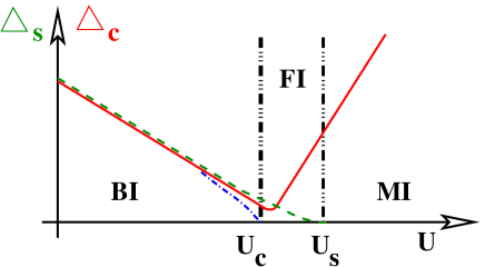
One important tool to characterize the different phases of the IHM is to study gaps to excited states, in particular making contact with the gaps obtained in the bosonization description. Following Ref. Man_04, we define the optical gap as the gap to the first excited state in the sector with the same particle number $N$ and with $S_{z}=0$, where $S_{z}$ is the $z$-component of the total spin. The single particle gap is determined as the difference in chemical potential for adding and subtracting one particle. Finally the spin gap is defined as the energy difference between the ground state and the lowest lying energy eigenstate in the $S=1$ subspace.

In Fig. 2 we present a qualitative sketch of the behavior of the single particle charge (solid line), spin (dashed line) and optical (dashed-dotted line) gap as a function of the on-site repulsion $U$ based on the exact numerical results obtained in Ref. Brune_03, and Ref. Man_04, . Two different sectors of the phase diagram corresponding to the BI and MI are clearly shown. These sectors are distinguished by the pronounced difference in the $U$ dependence of the charge excitation (single-particle excitation) gap.

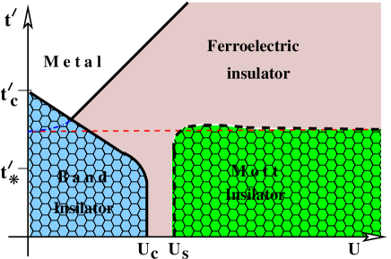
Below we treat the ground state phase diagrams of the IHM and of the noninteracting ionic-chain as border lines of our model. We explore the different character of the excitation gap renormalization by the Hubbard repulsion $U$ and consider the ground state phase diagram of the half-filled repulsive $t-t^{\prime}$ ionic-Hubbard chain. The key component of our analysis is based on the assumption that for arbitrary $U$ the infrared properties of the model are determined by the relation between the controlled effective chemical potential $\mu_{eff}$ and the value of the charge excitation gap. Moreover, in each charge gapped sector of the phase diagram, there is only one energy scale which is given either by the ionic distortion or by the Hubbard repulsion. This allows us to get the qualitative ground state phase diagram, which is summarized in Fig. 3.

At $t^{\prime}<t^{\prime}_{\ast}$ (i.e. $\mu_{\text{eff}}=0$) the ground state phase diagram remains qualitatively the same as at $t^{\prime}=0$: the BI phase is separated from a MI phase via a narrow stripe of the FI phase.

At $\mu_{\text{eff}}\neq 0$, but $t^{\prime}<t^{\prime}_{c}$ the BI phase is present for weak repulsion. With increasing $U$ the band-gap reduces, which simultaneously leads to a renormalization of the effective chemical potential $\mu^{r}=2(t^{\prime}-t^{\prime}_{r})$, where $t^{\prime}_{r}$ is given by (4) with $\Delta=\Delta_{r}$. Here we have to consider two cases separately.

At $t^{\prime}_{\ast}<t^{\prime}<0.5t$, the renormalized value of the chemical potential always remains less then the renormalized single-particle gap $\Delta_{r}/2$. Therefore with increasing $U$ the phase diagram is qualitatively the same as at $t^{\prime}<t^{\prime}_{\ast}$, i.e. with increasing $U$ the system undergoes a transition into a FI phase and with further increase of $U$ into a MI phase. Since the effective single band gap for $t^{\prime}_{\ast}<t^{\prime}$ is smaller than the single-particle gap at $t^{\prime}=0$, the transition from a BI into the FI insulator takes place for smaller $U$, which manifests itself in an extension of the FI phase in the direction of lower $U$.

At $0.5t<t^{\prime}<t^{\prime}_{c}$ the BI phase is still realized at weak $U$, but with increasing repulsive interaction one reaches the critical point $U_{c1}$, where the renormalized value of the chemical potential exceeds the renormalized single-particle gap $\Delta_{r}/2$. Neglecting quadratic corrections in $\Delta/t$, using (41) we easily find that $U_{c1}\simeq U^{\ast}[1-8(t^{\prime}-0.5t)/\Delta]\ll U^{\ast}\,.$ At $U>U_{c1}$ the BI phase is destroyed, the amplitude of the basic frequency field operator $\sin(\sqrt{2\pi}\varphi_{c})$ in the charge Hamiltonian (37) vanishes and the charge sector of the model is given by the Hamiltonian

$${\cal H}_{c} = \int dx\Big{\{}\frac{v_{c}}{2}\big{[}(\partial_{x}\varphi_{c})^{2}+(\partial_{x}\vartheta_{c})^{2}\big{]}$$ (42)

$$-\mu_{\text{eff}}\sqrt{\frac{2K_{c}}{\pi}}\partial_{x}\varphi_{c}-\frac{M_{c}}{2\pi^{2}a_{0}^{2}}\cos(2\sqrt{2\pi K_{c}}\varphi_{c})\Big{\}}\,.$$

The Hamiltonian (42) is a Hamiltonian which describes the charge sector of the $t-t^{\prime}$ Hubbard chain at $t^{\prime}>0.5t$ and contains two regimes of behavior:JNB_06

a) if the effective chemical potential is larger than the value of the correlated (Mott) gap at the transition point $\mu_{\text{eff}}>M_{c}(U_{c1})$ then the BI phase undergoes a transition into a charge gapless metallic phase. Since in the BI phase the energy scale of the model is given by the renormalized band-gap, in analogy with the non-interacting case of ionic chain we expect that the transition from a BI to a metal belongs to the universality class of commensurate-incommensurate transitions.

b) if $\mu_{\text{eff}}<M_{c}(U_{c1})$ then the BI phase undergoes a transition into a charge gapped ferroelectric phase.

We estimate the charge gap for $U\ll t$ as $M_{c}\approx\sqrt{Ut}e^{-2\pi t/U}$ and as $M_{c}\approx U$ for $U\gg t$. One finds that for $t^{\prime}\leq t^{\prime}_{c}$ the effective chemical potential is larger than the exponentially small Hubbard gap $M_{c}(U_{c1})$ and therefore for $0.5t<t^{\prime}<t^{\prime}_{c}$ there opens a window for a transition from the BI to a metallic phase with increasing on-site repulsion. With further increase of the on-site repulsion, at $U_{c2}$, when $M_{c}(U_{c2})=\mu_{\text{eff}}$ a charge gap opens once again, and for $U>U_{c2}$ the system is in the insulating ferroelectric phase (see Fig.3).

Figure 3: Qualitative sketch of the ground state phase diagram of the $t-t^{\prime}$ ionic-Hubbard chain in the case of repulsive interaction. Solid lines mark the phase transitions.

At $t^{\prime}>t^{\prime}_{c}$ the phase diagram is more simple. Already for $U=0$ the ground state corresponds to a metallic state, since the effective chemical potential is larger than the band-gap. With increasing Hubbard repulsion a transition into an insulating phase takes place, when the correlated gap $M_{c}$ becomes larger than the effective chemical potential. We expect, that similar to the usual $t-t^{\prime}$ model the transition from a metal to insulator belongs to the universality class of Kosterlitz-Thouless transitions.AebBaerNoack_01

Let us now briefly comment on the behavior of the spin sector. Is is usefull first to consider the strong coupling limit $U\gg\Delta,t,t^{\prime}$. In this limit the low-energy physics of the $t-t^{\prime}$ ionic-Hubbard chain is described by the spin $S=1/2$ frustrated Heisenberg model

$$H_{eff}=J\sum_{n}{\bf S}_{n}\cdot{\bf S}_{n+1}+J^{\prime}\sum_{i}{\bf S}_{n}\cdot{\bf S}_{n+2}\,,$$ (43)

where the exchange couplings are given by

$$J=\frac{4t^{2}}{U}\frac{1}{1-\Delta^{2}/U^{2}},\qquad J^{\prime}=\frac{4t^{\prime 2}}{U}\,.$$ (44)

For next-nearest neighbor couplings $J^{\prime}<0.25J$ the spin excitation spectrum of the spin model (43) is gapless and gapped for $J^{\prime}>0.25J$.Haldane Using (44) we easily conclude that at $t^{\prime}>0.5t$ and $U\gg t,\Delta$ a spin gapped spontaneously dimerized phase is realized in the ground state. Since for arbitrary finite alternating ionic potential the ground state of the system is characterized by the presence of a long-range ordered CDW pattern,Brune_03 we conclude that the whole charge and spin gapped sector of the phase diagram at $t^{\prime}>0.5t$ corresponds to a ferroelectric insulating phase. At $t^{\prime}<0.5t$ and for strong repulsion the spin sector is gapless and therefore in this limit a Mott insulating phase is realized. Note, that since the ionic potential slightly enhances the exchange parameter $J$ and does not influence (in first order with respect to $t^{2}/U$) the next-nearest-neighbor exchange $J^{\prime}$ for intermediate values of the on-site repulsion $U\geq 4t$, the Mott phase slightly penetrates into the $t^{\prime}>0.5t$ sector of the phase diagram.

In the weak-coupling limit at $t^{\prime}>0.5t$ the FI phase undergoes a transition either to the metallic phase or directly to the BI phase. Since the metallic phase with four Fermi points is characterized by a gapped spin sector for arbitrary weak on-site repulsionBalentsFisher_96 ; Fabrizio_96 ; DaulNoack_00 we conclude that the spin gapped phase is a generic feature of the model for $t^{\prime}>0.5t$. For $t^{\prime}<0.5t$, with increasing $U$ the spin gap continuously decays and finally vanishes in the MI phase.

To conclude our analysis we briefly discuss the phases which are realized along the transition lines. The border line between the BI and metallic phases corresponds to the Luttinger liquid state with gapless charge and spin excitation spectrum. The border line between the metallic and FI phases corresponds to the unconventional metallic phase with gapped spin and completely gapless charge excitation spectrum. The border line between the BI and FI phases corresponds to the unconventional metallic phase with gapless optical excitations and gapped spin and single-particle charge excitations. Finally, the border line between the FI and MI phases corresponds to the phase with gapped charge and gapless spin excitation spectrum.

IV Conclusions

We have studied the ground state phase diagram of the half-filled one-dimensional $t-t^{\prime}$ ionic-Hubbard model using the continuum-limit bosonization approach. We have shown that the gross features of the ground state phase diagram and in particular the behavior of the charge sector can be described by a quantum double-frequency sine-Gordon model with topological term. We have shown that with increasing on-site repulsion, for various values of the parameter $t^{\prime}$, the model shows the following sequences of phase transitions: Band insulator – Ferroelectric Insulator – Mott Insulator; Band Insulator – Nonmagnetic Metal – Ferroelectric Insulator and Nonmagnetic Metal – Ferroelectric Insulator.

We expect, that the transition sequence BI-metal-FI found in this paper is an intrinsic feature not only of the 1D chain, but is a generic feature of the $t-t^{\prime}$ ionic-Hubbard model and will show up also in higher spatial dimensions.

V Acknowledgments

It is our pleasure to thank D. Baeriswyl, F. Gebhard, D. Khomskii, R. Noack, A. Rosch and A.-M. Tremblay for many interesting discussions. GIJ and EMH acknowledge support from the research program of the SFB 608 funded by the DFG. GIJ also acknowledges support from the STCU-grant N 3867.

References

- (1)
- (2) N. F. Mott, Metal-Insulator Transitions, ed., Taylor and Francis, London (1990).
- (3) F. Gebhard, The Mott Metal–Insulator Transition, Springer, Berlin (1997).
- (4) M. Imada, A. Fujimori, and Y. Tokura, Rev. Mod. Phys. 70, 1039 (1998).
- (5) For a recent review see F. H. L. Essler, H. Frahm, F. Göhmann, A. Klümper, and V. E. Korepin, The One-Dimensional Hubbard Model, Cambridge Univ. Press, Cambridge (2005).
- (6) A. Rosch, Preprint arXiv Condmat/0602656.
- (7) F. Anfuso and A. Rosch, Preprint arXiv Condmat/0609051.
- (8) A. Fuhrmann, D. Heilmann, and H. Monien, Phys. Rev. B 73, 245118 (2006).
- (9) M. Fabrizio, A. O. Gogolin, and A. A. Nersesyan, Phys. Rev. Lett 83, 2014 (1999); ibid, Nucl. Phys. B 580, 647 (2000).
- (10) A. P. Kampf, M. Sekania, G. I. Japaridze, and P. Brune, J. Phys. C 15, 5895 (2003).
- (11) S. R. Manmana, V. Meden, R. M. Noack, and K. Schönhammer, Phys. Rev. B 70, 155115 (2004).
- (12) H. Otsuka and M. Nakamura, Phys. Rev. B 71, 155105 (2005).
- (13) M. E. Torio, A. A. Aligia, G. I. Japaridze, and B. Normand, Phys. Rev. B 73, 115109 (2006).
- (14) A. Garg, H. R. Krishnamurthy and M. Randeria, Phys. Rev. Lett. 97, 046403 (2006).
- (15) P. Lombardo, R. Hayn and G. I. Japaridze, Phys. Rev. B 74, 085116 (2006).
- (16) S.S. Kancharla and E. Dagotto, Preprint ArXiv Condmat/0607568.
- (17) M. E. Torio, A.A. Aligia, and H. A. Ceccatto, Phys. Rev. B 64, 121105(R) (2001).
- (18) A. A. Aligia, Phys. Rev. B 69, 041101(R) (2004).
- (19) A. A. Aligia, K. Hallberg, B. Normand, and A. P. Kampf, Phys. Rev. Lett. 93, 076801 (2004).
- (20) C. D. Batista and A. A. Aligia, Phys. Rev. Lett. 92, 246405 (2004); ibid, Phys. Rev. B 71, 125110 (2005).
- (21) N. Paris, K. Bouadim, F. Hebert, G.G. Batrouni, and R.T. Scalettar, Preprint arXiv Condmat/0607707
- (22) J. Hubbard and J.B. Torrance, Phys. Rev. Lett. 47, 1750 (1981); N. Nagaosa and J. Takimoto, J. Phys. Soc. Jpn. 55, 2735 (1986): T. Egami, S. Ishihara, and M. Tachiki, Science 261, 1307 (1993).
- (23) V. J. Emery, in Highly Conducting One-Dimensional Solids, edited by J. T. De Vreese, R. P. Evrard and V. E. Van Doren (Plenum, New York, (1979); J. Solyom, Adv. Phys. 28, 201 (1979).
- (24) A very exceptional case is the 1D electron system with the short-range (SR) and long-range (LR) Coulomb interaction. As was shown in Ref. PYMD_97, , in the case of commensurate band-filling and SR interaction which support the formation of a charge-density-wave (CDW) insulating phase, the increasing LR component of the Coulomb repulsion drives a transition from the CDW insulator to a metal. Further increase of the LR component leads to a transition from the metalic phase into the insulating Wigner crystal phase.
- (25) D. Poilblanc, S. Yunoki, S. Maekawa and E. Dagotto, Phys. Rev. B 56, R1645 (1997).
- (26) F. D. M. Haldane, Phys. Rev. B 25, 4925 (1982); ibid, 26, 5257 (1982).
- (27) K. Okamoto and K. Nomura, Phys. Lett. A 169, 422 (1992); S. Eggert, Phys. Rev. B 54, 9612 (1996).
- (28) S. R. White and I. Affleck, Phys. Rev. B 54, 9862 (1996).
- (29) R. Resta and S. Sorella, Phys. Rev. Lett. 74, 4738 (1995); ibid, Phys. Rev. Lett. 82, 370 (1999).
- (30) N. Gidopoulos, S. Sorella, and E. Tosatti, Eur. Phys. J. B 14, 217 (2000).
- (31) Y.Z. Zhang, C.Q. Wu, and H.Q. Lin, Phys. Rev. B 67, 205109 (2003).
- (32) M. Fabrizio, Phys. Rev. B 54, 10054 (1996).
- (33) K. Kuroki, R. Arita, and H. Aoki, J. Phys. Soc. Japan 66, 3371 (1997).
- (34) S. Daul and R. M. Noack, Phys. Rev. B 58, 2635 (1998).
- (35) R. Arita, K. Kuroki, H. Aoki, and M. Fabrizio, Phys. Rev. B 57, 10324 (1998).
- (36) S. Daul and R. M. Noack, Phys. Rev. B 61, 1646 (2000).
- (37) C. Aebischer, D. Baeriswyl, and R. M. Noack, Phys. Rev. Lett. 86, 468 (2001).
- (38) K. Louis, J. V. Alvarez and C. Gros, Phys. Rev. B 64, 113106 (2001); ibid, 65, 249903E (2002).
- (39) K. Hamacher, C. Gros, and W. Wenzel, Phys. Rev. Lett. 88, 217203 (2002).
- (40) M. E. Torio, A. A. Aligia, and H. A. Ceccatto, Phys. Rev. Lett. 67, 165102 (2003).
- (41) C. Gros, K. Hamacher, and W. Wenzel, Europhys. Lett. 69, 616 (2005).
- (42) M. Capello, F. Becca, M. Fabrizio, S. Sorella, and E. Tosatti, Phys. Rev. Lett. 94, 026406 (2005).
- (43) G.I. Japaridze, R.M. Noack and D. Baeriswyl, unpublished, condmat/0607054.
- (44) L. Balents and M. P. A. Fisher, Phys. Rev. B 53, 12133 (1996).
- (45) A. O. Gogolin, A. A. Nersesyan, and A. M. Tsvelik, Bosonization and Strongly Correlated Systems, Cambridge Univ. Press, Cambridge (1998).
- (46) T. Giamarchi, Quantum Physics in One Dimension, Clarendon Press, Oxford (2004).
- (47) G. I. Japaridze and A. A. Nersesyan, JETF Pis’ma 27, 356 (1978); [JETP Lett. 27, 334 (1978)]; ibidem, J. Low Temp. Phys. 37, 95 (1979); V. L. Pokrovsky and A. L. Talapov, Phys. Rev. Lett. 42, 65 (1979); H. J. Schulz, Phys. Rev. B 22, 5274 (1980).
- (48) G. I. Japaridze, A. A. Nersesyan, and P. B. Wiegmann, Nucl. Phys. B 230, 511 (1984).
- (49) Al. B. Zamolodchikov, Int. Jour. Mod. Phys. A 10, 1125-1150 (1995).
- (50) S. Lukyanov, A. Zamolodchikov, Nucl.Phys. B 493, 571 (1997).
- (51) R.F. Dashen, B. Hasslacher and A. Neveu, Phys. Rev. D 10 3424 (1975); A. Takhtadjan and L.D. Faddeev, Sov. Theor. Math. Phys., 25, 147 (1975).
- (52) G. Delfino and G. Mussardo, Nucl. Phys. B 516, 675 (1998).
- (53) F. D. M. Haldane, Phys. Rev. B 25, 4925 (1982); K. Okamoto and K. Nomura, Phys. Lett. A 169, 433 (1993); G. Castilla, S. Chakravarty, and V. J. Emery, Phys. Rev. Lett. 75, 1823 (1995).