Smoothing a Rock by Chipping

Abstract

We investigate an idealized model for the size reduction and smoothing of a polygonal rock due to repeated chipping at corners. Each chip is sufficiently small so that only a single corner and a fraction of its two adjacent sides are cut from the object in a single chipping event. After many chips have been cut away, the resulting shape of the rock is generally anisotropic, with facet lengths and corner angles distributed over a broad range. Although a well-defined shape is quickly reached for each realization, there are large fluctuations between realizations.

I Introduction and Model

This work is inspired by a recent experiment of Durian et al. DD in which they were interested in the ultimate shape of eroding rocks. To investigate this issue quantitatively, they studied the collisional erosion of square clay particles due to their repeated impact with the walls of a horizontally rotating plane enclosure. In each such collision, chips break off from the particle so that it gradually becomes rounder and smoother. One might naively expect the asymptotic particle shape to be a circle, as protruding corners are more exposed and thus likelier to get rounded off by this grinding process.

Figure 1: Schematic illustration of the cutting model after 1, 2, 3, and 8 events. A chip breaks from a randomly-selected corner with the sum of the new deflection angles, $\theta_{1}$ and $\theta_{2}$ equal to the deflection angle $\theta$ of the previous corner. The geometry of a single chipping event is shown at the lower right.

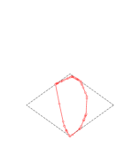
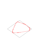
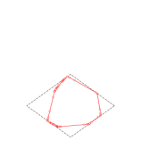
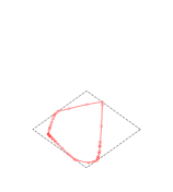
Figure 2: (Color online) Four typical realizations of the cutting model for an initial unit square (dashed) after 100 corners (circles).

A striking result from this experiment is that the asymptotic shape of the eroding rock is not a circle DD . To describe this unexpected shape evolution, Durian et al. also introduced a simple “cutting” model in which the material exterior to a random chord on the object, whose length is proportional to the square root of the remaining area, is removed in each cutting event. This step is repeated many times until asymptotic behavior is reached. Numerical simulations reproduced various aspects of the experimental observations and confirmed that the asymptotic shape of the particle is not circular DD .

In this work, we investigate an idealized and analytically tractable version of this cutting model. A sequence of chipping events in our model is schematically illustrated in Fig. 1. The rock is initially assumed to be square. In each chipping event, a piece of the rock is broken off at a corner. The deflection angles of the two newly-created corners sum to the deflection angle of the original corner but are otherwise arbitrary. The sides $z_{1}$ and $z_{2}$ of a chip are smaller than the respective sides $L_{1}$ and $L_{2}$ of the corner itself (lower right in Fig. 1), so that only a single corner and a finite fraction of its two adjacent sides are removed in each chipping event. As the rock is chipped away, a non-trivial shape is generated that is the focus of our interest.

A convenient geometrical representation for the evolution of corner deflection angles is to view the initial angle as a line segment of length $\pi/2$ (Fig. 3). Each chipping event then corresponds to picking one segment at random and cutting it into two arbitrary size pieces. This connection to binary fragmentation allows us to make use of well-known results for this latter problem ZM to help understand geometrical features of the object as its size is reduced by chipping.

Figure 3: Equivalence between angle evolution in chipping and fragmentation of a line segment.

The constraint that the chip breaks off only a single corner and a portion of its two adjacent sides ensures that final particle size is strictly positive; that is, the initial particle is not eroded to nothingness. This fact can be appreciated by examining Fig. 2. By the definition of the model, a short segment on each of the sides of the initial square must remain part of the perimeter of the eroding particle in the long time limit. This fact ensures that a particle of non-zero size remains in the long-time limit. Each of these four segments may be arbitrarily small and two such segments on adjacent sides of the initial square may be arbitrarily close to each other. In the exceptional case where short segments occur in pairs at opposite diagonals of the initial square, the area can be arbitrarily small, but with vanishing probability of the size being zero.

In the next section, we investigate the evolution of the distribution of facet angles by a master equation approach when each chipping event bisects the corner angle. We show that the resulting angle distribution has a Poisson form in the variable $\ln t$, where $t$ is the current number of corners. In Sec. III, we study the evolution of the angle distribution, as well as the actual shape of the object, for the general situation where a chip divides a corner angle $\theta$ into two arbitrary angles $\theta_{1}$ and $\theta_{2}$, with $\theta=\theta_{1}+\theta_{2}$. For this process, we find: (i) the asymptotic shape of an eroding particle is not round and (ii) after many chipping events, the particle is characterized by large sample-to-sample fluctuations. In Sec. IV, we investigate some natural extensions to more physical cutting rules and conclude that our main qualitative results are robust with respect to these generalizations. We close with a brief discussion in Sec. V.

II Angle Bisection

II.1 Master equation solution

We first treat the special case in which a corner angle is always bisected in each chipping event. As a result of repeated chipping events a non-trivial distribution of corner angles develops. Starting with the four right-angle corners of an initial square, after one chipping event, two angles of magnitude $\pi/4$ are created, while three right-angle corners remain. After a second event, either two more $\pi/4$ angles are created by chipping a right angle (this occurs with probability 3/5), or one $\pi/4$ angle is replaced by two new $\pi/8$ angles (this occurs with probability 2/5).

To determine the angle distribution, it is convenient to introduce the integer variable $k\equiv-\ln_{2}(2\theta/\pi)$. The initial angle $\pi/2$ then corresponds to $k=0$, and each angle halving corresponds to $k$ increasing by 1. We refer to a corner with deflection angle corresponding to $k$ as a $k$-corner. Let $n_{k}(t)$ be the average number of $k$-corners. Starting with a square, the initial condition is $n_{k}(t=0)=4\delta_{k,0}$ and the number of corners at time $t$ is simply $t+4$. Then the change in $n_{k}(t)$ after one chipping event obeys the master equation

$$n_{k}(t+1)-n_{k}(t)=\frac{2}{t+4}\,n_{k-1}(t)-\frac{1}{t+4}\,n_{k}(t)\,.$$ (1)

The first term on the right side accounts for the gain of $k$-corners due to the chipping of one of the $(k-1)$-corners at time $t$. The probability of this event is ${n_{k-1}}/(t+4)$, and each such event increases the number of $k$-corners by 2. Conversely, the second term accounts for the loss of $k$-corners when one such corner is chipped.

The system of master equations is recursive, and they can be solved one by one. Since $n_{-1}\equiv 0$, the average number of the 0-corners (right-angle corners) satisfies the closed equation

$$n_{0}(t+1)=\frac{t+3}{t+4}\,n_{0}(t).$$ (2)

Iterating this equation, the solution is

$$n_{0}(t)=\frac{12}{t+3}.$$ (3)

The average number of 1-corners satisfies

$$n_{1}(t+1)=\frac{t+3}{t+4}\,n_{1}(t)+\frac{2}{t+4}\,\frac{12}{t+3},$$ (4)

with solution (subject to the initial condition $n_{1}(0)=0$)

$$n_{1}(t)=\frac{24}{t+3}\sum_{3\leq j\leq t+2}\frac{1}{j}.$$ (5)

With the solution for $n_{1}$, the average number of 2-corners satisfies

$$n_{2}(t+1)=\frac{t+3}{t+4}\,n_{2}(t)+\frac{2}{t+4}\,\frac{24}{t+3}\sum_{3\leq j\leq t+2}\frac{1}{j},$$ (6)

whose solution is

$$n_{1}(t)=\frac{48}{t+3}\sum_{3\leq i<j\leq t+2}\frac{1}{i\,j}.$$ (7)

While these exact expression for $n_{k}$ become progressively unwieldy as $k$ increases, the asymptotic behavior follows easily by noticing that in the $t\to\infty$ limit the master equation (1) turns into a differential equation

$$\frac{dn_{k}}{dt}=-\frac{n_{k}}{t}+\frac{2}{t}\,n_{k-1}.$$ (8)

These equations can also be solved straightforwardly in a sequential manner. Using the fact that $n_{0}\sim{12}/{t}$ and rewriting (8) as

$$\frac{d(tn_{k})}{dt}=\frac{2(tn_{k-1})}{t},$$ (9)

we then obtain the solution

$$n_{k}(t)=\frac{12}{t}\,\frac{(2\ln t)^{k}}{k!}.$$ (10)

Thus the logarithm of the angle is a Poisson distribution with $\langle k\rangle=2\ln t$, corresponding to $\langle\theta\rangle\propto e^{-t}$.

While the final result for $n_{k}$ is quite simple, we emphasize that Eq. (10) refers to the number of $k$-corners averaged over all possible realizations of the cutting model. However, the actual number of $k$-corners in a given realization, defined as $N_{k}$, may differ substantially for $n_{k}\equiv\langle N_{k}\rangle$. In the appendix, we investigate some of the simplest features of the $N_{k}$ that illustrate their strongly fluctuating nature.

II.2 Simulation results

We simulated the probabilistic rules underlying the recursion formula (1) to obtain the distribution $N_{k}$ for each realization. This numerical approach has the advantages of simplicity and efficiency, but with the obvious disadvantage that the actual shape of the particle is not accessible by this approach.

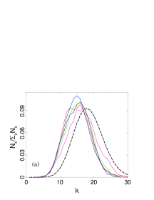
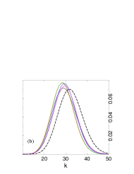
Figure 4: (Color online) Normalized distributions of corner angles, $N_{k}/\sum_{k}N_{k}$, versus $k$ for 5 realizations of $10^{4}$ corners (a) and $10^{7}$ corners (b). The heavy dashed curve is the properly normalized asymptotic expression from Eq. (10).

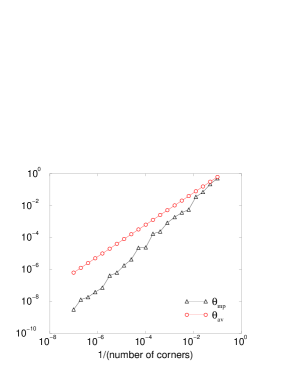
Figure 5: (Color online) Average and most probable angles for a single realization of the cutting process as a function of the number of corners.

The data show that the distribution of the logarithm of the angle (actually $k=-\ln(2\theta/\pi)$) is close a Poisson form in $k$, as predicted by Eq. (10). To compare the data with this analytic expression, however, we need to properly normalize the latter. Summing Eq. (10) over all $k$, one obtains $\sum_{k}n_{k}=12t$ for the total number of corners, whereas the exact result is $t+4$. To correct for this discrepancy, we therefore divide the expression in (10) by 12 to compare with the data in Fig. 4. The data are in reasonable agreement with the properly normalized analytic distribution, but it appears that one would have to simulate the chipping process for an astronomical number of corners to obtain good agreement between the data and the asymptotic expression.

Another important property of the angle distribution is the large difference between the average angle $\langle\theta\rangle$ and the most probable angle $\theta_{\rm mp}$. Because the distributions in Fig. 4 are plotted against $-\ln\theta$, it is clear that $\langle\theta\rangle$ is much larger than $\theta_{\rm mp}$, which is located at the peak of the distribution as shown in Fig. 5.

Finally, because the natural variable is $\ln\theta\,$ the actual angle distribution is very broadly distributed. Consequently, the asymptotic shape of a particle as a result of this cutting process will not be circular. A related feature is that simulation results from different realizations are visually quite different, as might be anticipated by the random multiplicative process that underlies the chipping process. We will discuss this feature in more detail in the next section.

III Arbitrary Chipping Angles

III.1 The angle distribution

We now study the general situation where a chipping event creates two unequal angles. To determine the resulting angle distribution, we make use of the geometric connection between chipping and binary fragmentation. As illustrated in Fig. 3, a corner angle $\theta$ that becomes two corners of angles $\theta_{1}$ and $\theta_{2}$ (with $\theta_{1}+\theta_{2}=\theta$), corresponds to the length-conserving cutting of a segment of length $\theta$ into two pieces of lengths $\theta_{1}$ and $\theta_{2}$. The angle distribution in chipping then corresponds to the length distribution in the equivalent fragmentation process.

The length distribution may be solved using the techniques from the theory of fragmentation ZM . For convenience, consider the scaled segment length $x\equiv 2\theta/\pi$. Starting with a segment of scaled length $x=1$, the master equation for the length distribution is

$$\begin{split}\frac{\partial c(x,t)}{\partial t}=-c(x,t)\int_{0}^{x}&F(y,x-y)\,dy\\ &+2\int_{x}^{1}c(y,t)F(x,y-x)\,dy.\end{split}$$ (11)

Here $c(x,t)$ is the concentration of fragments of length $x$ at time $t$ and $F(x,y)$ is the rate at which a fragment of size $x+y$ is cut two pieces of sizes $x$ and $y$. The first term on the right accounts for the loss of fragments of size $x$ due to their fragmentation. The total rate of these events is $\int_{0}^{x}F(y,x-y)\,dy$. The second term on the right accounts for the creation of a fragment of size $y$ due to the breakup of a larger segment of size $y$.

In many fragmentation processes ZM ; CR , the breakup rate $F(x,y)$ is a homogeneous function of the form $F(x,y)=(x+y)^{\lambda-1}$. That is, the breakup rate of a cluster of size $x+y$ depends only on its size and not on the size of the two daughter fragments. To make a direct connection with cutting, we require $\lambda=0$ so that the total breaking rate of a fragment is independent of its size. In this case, the master equation becomes

$$\frac{\partial c(x,t)}{\partial t}=-c(x,t)+2\int_{x}^{1}c(y,t)\,\frac{dy}{y}.$$ (12)

This master equation represents the generalization of (9) to continuum angles.

For the initial condition corresponding to a square, $c(x,t=0)=4\delta(x-1)$, the distribution of unscaled fragment sizes at any later time is given by ZM

$$\begin{split}c(\theta,t)=\frac{8}{\pi}\sqrt{\frac{2t}{\ln(\pi/2\theta)}}&\,e^{-t}I_{1}\left(\sqrt{8t\ln(\pi/2\theta)}\right)\\ &+\frac{8}{\pi}e^{-t}\delta\Big{(}\theta-\frac{\pi}{2}\Big{)},\end{split}$$ (13)

where $I_{1}$ is a modified Bessel function of order 1. The second term on the right-hand side corresponds to the probability that there have been no fragmentation events up to time $t$, while the first term on the right gives the scaling part of the fragment size distribution.

From the variable combination in this first term, we find that the characteristic angle has the time dependence $\theta\sim e^{-t}$. Furthermore, from the asymptotic form of the Bessel function AS , the distribution of the logarithmic angle has a stretched exponential tail

$$c(x,t)\sim e^{\sqrt{-t\ln\theta}},$$

with $-\ln\theta$ being the natural variable of the system. As in the case of symmetric chipping (angle bisection), the general chipping process leads to a broad distribution of angles. This result again suggests that the asymptotic shape of the particle is not circular.

III.2 Shape Evolution

Area and Perimeter Distributions. Two fundamental characteristics of an object’s shape are its area and its perimeter. Starting with a unit-area square, the resulting area and perimeter distributions become smooth, sharply peaked about their average values, and visually independent of the number of corners $N$ when $N\gtrsim 20$. The support of the area distribution is $[0,1]$, with a peak near 0.67. Similarly, the support of the perimeter distribution is $[2\sqrt{2},4]$ and the peak occurs at approximately 3.3.

Figure 6: The distribution of (a) area and (b) perimeter after 50 corners for $10^{7}$ realizations.

An amusing unexplained feature is that a careful examination of the data reveals that the first derivatives of both distributions are actually discontinuous—the area distribution at area equal to 1/2 and perimeter distribution at scaled perimeter $p_{\rm scaled}\equiv({p-p_{\rm min}})/({p_{\rm max}-p_{\rm min}})$ also at $p_{\rm scaled}=1/2$.

Asymmetry and Fluctuations. After a particle has approximately 50 corners, a given realization is visually close to its asymptotic shape. As illustrated in Fig. 2, large fluctuations between different realizations arise, so that the shape of a single realization has little connection to the average shape.

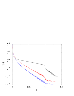
Figure 7: (Color online) Probability distribution of facet lengths $P(L)$ versus $L$ for $10^{5}$ realizations of 10, 40, and 80 corners. The steeper curve corresponds to larger $N$.

Each individual interface typically consists of a few longer facets that are punctuated by regions with many short facets, with a consequent large change in the local tangent. To illustrate this punctuated interface, we show the facet length distribution for $10^{5}$ realizations with $N=10,40$, and 80 corners (Fig. 7). The spike at $L=1$ corresponds to the initial unit-length facets that remain unchipped. The tail for $L>1$ corresponds to an initial cut that is sufficiently close to the main diagonal of the initial square so that the facet length can be greater than 1—in fact, the maximal facet length is $\sqrt{2}$. This large-$L$ tail is distinct from the rest of the distribution when the number of corners is small. As the number of corners increases, the number of short facets correspondingly increases, and there is a huge buildup of the small-length tail of the facet length distribution.

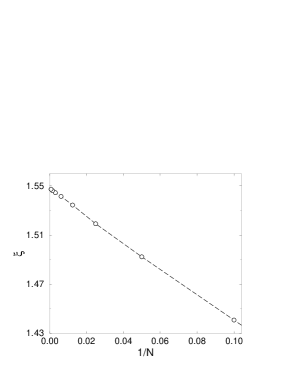
Figure 8: Asymmetry ratio $\xi(N)\equiv\sqrt{\langle R_{+}^{2}(N)\rangle}/\sqrt{\langle R_{-}^{2}(N)\rangle}$ versus $1/N$. Each data point is based on $10^{6}$ realizations, with $N=10,20,\ldots,1280$.

Finally, we study how the asymmetry of the particle evolves during the cutting process. The proper measure of asymmetry is through the moment of inertia tensor of an object. For the cutting model, this leads to a cumbersome calculation when the number of corners is large. We therefore adopt a simpler approach that should reveal the same type of information as the inertia tensor. After an initial square has been reduced to an object with a specified number of corners $N$, we determine the $x$- and $y$-coordinates of each corner about the center of the initial square and then compute the mean-square displacements of the $x$- and $y$-coordinates of all the corners

$$X^{2}(N)=\frac{1}{N}\sum_{i=1}^{N}x_{i}^{2}\qquad Y^{2}(N)=\frac{1}{N}\sum_{i=1}^{N}y_{i}^{2}$$

in each realization. For each realization we then define the larger and the smaller of these two mean-square displacements,

$$R_{+}^{2}(N) ={\rm max}(X^{2}(N),Y^{2}(N))$$

$$R_{-}^{2}(N) ={\rm min}(X^{2}(N),Y^{2}(N)),$$

and then average these maximal and minimal mean-square radii over many realizations. Finally, we quantify the asymmetry by the dimensionless ratio

$$\xi(N)\equiv\sqrt{\langle R_{+}^{2}(N)\rangle}/\sqrt{\langle R_{-}^{2}(N)\rangle}.$$

Thus, for example, a rhombus in which the two corners in the $x$-direction are a unit distance from the origin while the other two corners are a distance $1+\epsilon$, $\xi=(1+\epsilon)$. As a function of $1/N$, the data for $\xi(n)$ are quite linear for $N$ between 10 and 1280. Extrapolating the data of Fig. 8 to $1/N\to 0$, we infer the value of $\xi(N\to\infty)\approx 1.548$, with a subjective uncertainty of 0.001.

IV Extensions of the Model

An unrealistic feature of our cutting model is that each corner has the same probability of being chipped. As a consequence, corners tend to congregate, as seen in Fig. 2. In the equivalent fragmentation process, equiprobable corner chipping corresponds to an overall breakup rate for a given segment that is independent of its length. This length-independent breakup rate in fragmentation demarcates the boundary between scaling solutions, when the breakup rate grows with segment length, and “shattering” solutions ZM ; CR , when the breakup rate decreases with segment length. The shattering solution is characterized by a finite fraction of the system being transformed into a dust of zero-length particles that contain a finite fraction of the initial length. This singularity is parallel to the gelation transition in irreversible aggregation.

Thus a natural question is whether different behavior arises in the physically more realistic situation in which larger protrusions are likelier to be chipped. In the language of the equivalent fragmentation process, we should study break-up rates with a positive homogeneity index—namely, larger fragments are more likely to break. To study the role of a positive homogeneity index, we considered the extreme situation in which only the most susceptible corner breaks in a chipping event. We thus investigated the following three extremal dynamics rules:

1. Chip the corner furthest away from the origin.

2. Chip one of the corners on the longest facet.

3. Chip the corner with the largest deflection angle.

Each of these chipping rules focuses on some aspect of the most prominent non-smooth regions of the object. Qualitatively, we find that these three rules all lead to a non-circular asymptotic shape of the object. The reason for this non-circularity ultimately stems from the strong role played by the first few chipping events. The size of each chip can, in principle, range from zero to its maximum attainable size (see Fig. 1). If one of these early chips is close to its maximal size, this chip leaves an imprint on the object that persists in the long-time limit. This property is different than that of curvature-driven interface evolution, in which the amount by which a curved region of the interface moves is strictly proportional to the local curvature curvature .

Figure 9: Geometry of a two-corner chipping event.

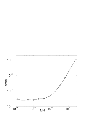
Figure 10: Average area of a unit square after $N$ cuts versus $1/N$ on a double logarithmic scale when the probability of 2-corner chipping $p_{2}=0.9$.

Another natural concern about the applicability of the cutting model is the restriction to breaking only a single corner and portions of its adjacent sides in a single chipping event. Indeed this rule ensures that the final size of the particle remains non zero as mentioned in the introduction. To test the robustness of the cutting model results to the possibility that more than one corner can be chipped away, we studied the situation in which a chip could encompass two corners, as illustrated in Fig. 9. Specifically, we pick a corner at random; with probability $p_{2}$, the chip includes both this corner and its nearest neighbor. With this rule, the restriction that a small segment of the initial square must remain as part of the boundary of the eroding particle no longer applies. Thus it is not obvious a priori that the size of the object will remain non-zero in the long-time limit. Nevertheless, this more generous two-corner chipping rule still leads to a non-zero particle size, as long as the probability for single-corner chips is non-zero. Initially, the area decreases rapidly as the number of cuts increases. However, As the number of corners becomes appreciable, later cuts remove only a tiny fraction of the particle so that the area eventually saturates to a non-zero value (Fig. 10).

V Discussion

We studied the geometric properties of an idealized model for the erosion of a two-dimensional rock by repeated chipping of small pieces. A chipping event is defined by cutting a small piece from the rock in which a single corner and part of its two adjacent sides are removed. In our model, each corner has the same probability of being chipped. A two basic outcome of this cutting model is that there is shape asymmetry in the long-time limit. Thus the asymptotic outcome after many chipping events is not a circle, as was initially observed in the experiments and the simulations of Durian et al. DD . Another important feature is that there are large shape fluctuations between realizations so that the outcome of a single event is not representative of the average behavior.

We determined the evolution of the distribution of angles from its governing master equation. For the case of angle bisection in each chipping event, we found a broad and asymptotically Poissonian distribution of angles in the variable in $\ln t$, where $t$ is the number of chipping events. This behavior appears to be idiosyncratic to the case of angle bisection. In the more realistic case where a chipping event divides an initial angle into two arbitrary angles (with conservation of the total angle), the angle distribution has a different behavior that is immediately obtained by the exact correspondence between the distribution of angles in the cutting model and the distribution of fragments sizes in the binary fragmentation of a line segment ZM ; CR .

Finally, it is worth mentioning that because of large sample-to-sample size and shape fluctuations after a given number of chipping events, the cutting model does not give a unique limiting shape. This behavior is in contrast to the class of interface models where the asymptotic shape of a single realization of interface converges to a unique limiting shape. Two famous such examples are the strictly convex interface between the origin and $(x\gg 0,y\gg 0)$ segment and the interface that is generated by the partition of the integers partition . It may be worthwhile to explore variants of the cutting model that lead to a unique limiting shape to take advantage of the highly-developed analysis methods available for this type of interface evolution process. It should also be of interest to extend our study to the more realistic case of three dimensions, where there is also a highly-developed mathematical literature on limiting shapes 3d .

Appendix A Fluctuations in $n_{k}$

In this appendix we investigate the statistical properties of the distribution of $k$-corners in greater detail. We show that the actual value of the number of $k$-corners in a given realization, $N_{k}$, is generally quite different than the average number of $k$-corners, $n_{k}$. This lack of self averaging can be seen by studying the probability distribution of the random quantities $N_{k}(t)$ across all realization. While the full calculation is a tedious endeavor, it is fairly simple to obtain the number of right-angle corners $N_{0}(t)$. The master equation for $N_{0}$ is simpler than that for all the other $N_{k}$ with $k>0$, because $N_{0}$ can never increase in a single chipping event.

Starting with a square that has four right-angle corners, the number of such corners is a deterministic quantity when $t=0$ and $t=1$,

$$N_{0}(0)=4,\quad N_{0}(1)=3,$$

while for $t>1$ the number of right-angle corners is a random quantity. Let

$$\Pi_{j}(t)\equiv{\rm Prob}\{N_{0}(t)=j\},$$

and let us compute $\Pi_{j}(t)$ for $t>1$.

We begin with $\Pi_{3}(t)$. To have three right-angle corners, each chipping event must not act on any of these corners. Consequently, the probability to have three right-angle corners satisfies the recurrence

$$\Pi_{3}(t+1)=\frac{t+1}{t+4}\,\Pi_{3}(t).$$ (14)

Solving this recurrence subject to the initial condition $\Pi_{3}(1)=1$ we obtain

$$\Pi_{3}(t)=\frac{24}{(t+1)(t+2)(t+3)}.$$ (15)

By similar reasoning, the recurrence for the probability to have two right-angle corners is

$$\Pi_{2}(t+1)=\frac{t+2}{t+4}\,\Pi_{2}(t)+\frac{3}{t+4}\,\Pi_{3}(t),$$ (16)

whose solution is

$$\Pi_{2}(t)=\frac{36(t-1)}{(t+1)(t+2)(t+3)}.$$ (17)

The probability to have a single right-angle corner satisfies the recurrence

$$\Pi_{1}(t+1)=\frac{t+3}{t+4}\,\Pi_{1}(t)+\frac{2}{t+4}\,\Pi_{2}(t),$$ (18)

from which

$$\Pi_{1}(t)=\frac{12(t-1)(t-2)}{(t+1)(t+2)(t+3)}.$$ (19)

Finally the probability that there are no right-angle corners can be found by solving the appropriate recurrence formula

$$\Pi_{0}(t+1)=\Pi_{0}(t)+\frac{1}{t+4}\,\Pi_{1}(t),$$ (20)

or from the normalization $\Pi_{0}+\Pi_{1}+\Pi_{2}+\Pi_{3}=1$. In either case, we obtain

$$\Pi_{0}(t)=\frac{(t-1)(t-2)(t-3)}{(t+1)(t+2)(t+3)}$$ (21)

As a useful consistency check one can compute

$$n_{0}=\langle N_{0}\rangle=\sum j\Pi_{j}\,$$

and recover the result $n_{0}=\frac{12}{t+3}$ given in Eq. (3).

References

- (1) D.J. Durian, H. Bideaud, P. Duringer, A. Schroder, F. Thalmann, and C.M. Marques, Phys. Rev. Lett. 97, 028001 (2006); D.J. Durian, H. Bideaud, P. Duringer, A. Schroder, and C.M. Marques, cond-mat/0607122.
- (2) R. M. Ziff and E. D. McGrady, J. Phys. A 18, 3027 (1985); R. M. Ziff, J. Phys. A 25, 2569 (1992).
- (3) Z. Cheng and S. Redner, Phys. Rev. Lett. 60, 2450 (1988); J. Phys. A 23, 1233 (1990).
- (4) M. Abramowitz and I. A. Stegun Handbook of Mathematical Functions (Dover, New York, 1972).
- (5) W. W. Mullins, J. Appl. Phys. 27, 900 (1956); G. Huisken, J. Diff. Geom. 20, 237 (1984); M. E. Gage and R. S. Hamilton, J. Differential Geom. 23, 69 (1986); M. A. Grayson, J. Diff. Geom. 26, 285 (1987); D. L. Chopp and J. A. Sethian, Exp. Math. 2, 235 (1993); D. L. Chopp, Exp. Math. 3, 1 (1994).
- (6) A. Vershik, Func. Anal. Appl. 28, 13 (1994); Ya. G. Sinai, Func. Anal. Appl. 28, 108 (1994).
- (7) A. Vershik, Func. Anal. Appl. 30, 90 (1996); S. Shlosman, J. Math. Phys. 41, 1364 (2000); P. L. Krapivsky, S. Redner, and J. Tailleur, Phys. Rev. E 69, 026125 (2004); R. Rajesh and D. Dhar, Phys. Rev. E 71, 016130 (2005).
- (8) A. Okounkov and N. Reshetikhin, J. Am. Math. Soc. 16, 581 (2003); A. Okounkov and N. Reshetikhin, Commun. Math. Phys. 269, 571 (2007); R. Kenyon and A. Okounkov, math-ph/0507007.