Kinetics and mechanism of proton transport across membrane nanopores

Abstract

We use computer simulations to study the kinetics and mechanism of proton passage through a narrow–pore carbon–nanotube membrane separating reservoirs of liquid water. Free energy and rate constant calculations show that protons move across the membrane diffusively in single-file chains of hydrogen-bonded water molecules. Proton passage through the membrane is opposed by a high barrier along the effective potential, reflecting the large electrostatic penalty for desolvation and reminiscent of charge exclusion in biological water channels. At neutral pH, we estimate a translocation rate of about 1 proton per hour and tube.

Long-range proton transfer is central to processes as diverse as hydrogen fuel cells Paddison ; Weber_Newman , the enzymatic function of many proteins, and in particular membrane biophysics HilleBook . To explore the fundamental question of water-mediated proton transfer, and to design robust proton conducting media for technological applications, studying simpler model systems is essential. The quasi-one-dimensional water chains forming inside carbon nanotubes GH_NATURE have attracted considerable attention, with computer simulations suggesting proton mobilities exceeding those even of bulk water POMES_ROUX1 ; MEI ; VOTH_WIRE ; DellagoPRL ; HallPRL ; HassanJCP . However, large conductivity requires in addition a high density of charge carriers, which depends on the free energy penalty required to remove protons from the bulk liquid and introduce them into the pores. This then raises the question if water-filled nanotubes can actually carry protonic currents of high density, i.e., whether the electrostatic desolvation penalty of the proton is compensated, at least in part, by its exceptionally high mobility.

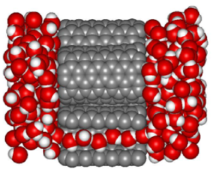
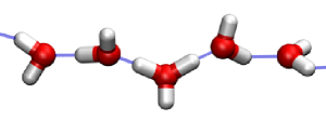
Figure 1: (color online). Top: Side view of the carbon nanotube membrane immersed in liquid water. One carbon nanotube is cut open to expose the chain of hydrogen bonded water molecules traversing the pore. Bottom: Enlarged view of a typical configuration of a protonic defect in the water chain inside the pore.

Here, we will use computer simulations to explore the kinetics and mechanism of proton translocation through nanopores. In our simulations, four rigid (6,6) armchair-type carbon nanotubes of 144 carbon atoms each are packed into a hexagonal array to form a nanotube membrane in the periodically replicated simulation box (Fig. 1). The size of the simulation box in the $z$–direction parallel to the tube axes is $34.3$ Å, and $22.5$ Å and $19.5$ Å, respectively, in the $x$– and $y$–directions. The membrane is immersed in a bath of 292 water molecules containing one excess proton. At $T=300$ K and a density corresponding to that of liquid water, the $\sim$8-Å diameter pores fill with single-file chains of six hydrogen bonded water molecules. In our simulations, the equations of motion are integrated with the velocity Verlet algorithm using a time step of 0.489 fs and a hydrogen mass of 2 a.m.u. For the interactions of the water molecules and the excess proton, we use the multistate empirical valence bond model (EVB) developed by Voth and collaborators VOTH based on prior work of Warshel WARSHEL_EVB . This model accurately describes the energetics of bond breaking and formation during aqueous proton transfer and is computationally far less expensive than ab initio methodologies DellagoPRL . The water oxygen atoms interact with the carbon atoms of the nanotube through a Lennard-Jones potential with $\epsilon=0.1143$ kcal/mol and $\sigma=3.27$ Å yielding a channel aperture of approximately 2 Å. Periodic boundary conditions with Ewald sums for the Coulombic interactions apply in all three spatial directions. We stress that the model and setup used here does not bias the simulation towards a particular H⁺ transport mechanism.

In the bulk liquid outside the carbon nanotube membrane the excess proton moves primarily as a high mobility charge defect by proton transfers along the hydrogen bond network percolating through the liquid. During this so-called Grotthuss-process, the hydrated proton exists in a continuum of structures including as the limiting cases the Eigen cation H₉O${}_{4}^{+}$, consisting of a hydronium ion H₃O⁺ tightly hydrogen-bonded to three neighboring water molecules, and the Zundel cation H₅O${}_{2}^{+}$, in which the excess proton is shared between two water molecules AGMON ; MARX ; AGMON_VOTH . This structural diffusion process is rapid with typical proton hopping times on the picosecond timescale such that during the nanosecond simulations of this study each water molecule outside the membrane is visited several times by the excess charge. During these simulations, however, the proton never entered the membrane pores.

To clarify what prevents the proton from penetrating into the membrane interior despite the high proton mobility along one-dimensional water chains DellagoPRL we have calculated the free energy profile $F(z)$ for the excess charge as a function of its position $z$ along the tube axis as shown in Fig. 2. We computed the free energy $F(z)$ inside the pore ($|z|\leq 7.4$ Å) using umbrella sampling Monte Carlo simulations in 10 separate windows. New configurations were generated with path sampling moves DBCC98 ; tps_review2 . In each window a total of 30,000 path shooting and shifting moves of 14.6 fs long trajectory segments were carried out amounting to a total simulation time of about 350 ps per window. Within the windows the free energy $F(z)$ was determined from the histogram $P(z)$ of the position of the center of charge EVB_NEW , essentially the position of the hydronium ion averaged over all EVB states. The overall free energy profile was obtained by matching the free energies calculated in the separate windows and the 2.2 ns equilibrium run.

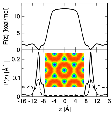
Figure 2: Top: (color online). Free energy profile for the center of charge along $z$, where $z=0$ corresponds to the tube center. Bottom: Corresponding probability distribution of the excess charge (solid line) and a particular water oxygen (dashed line). The inset shows the $xy$-projected probability density of the protonic defect in a slab $7{\rm\AA}<|z|<11{\rm\AA}$ just outside the carbon nanotube membrane, obtained from a molecular dynamics simulation of 2 ns. Red color indicates low proton density and blue high proton density. The rims of the carbon nanotubes are visible as red circles.

Coming from the bulk, the free energy $F(z)$ first decreases, goes through a minimum at $|z|\approx 10$ Å, and then rises almost linearly, reaching an approximately flat and 8 Å-wide top near the tube center. The total free energetic cost of moving the excess charge from the bulk phase to the tube center is $\sim$10 kcal/mol, about 1/3 the cost for a sodium ion in a similar system Peter:BJ:2005 . As the motion of a proton along an isolated hydrogen bonded water chain is an essentially barrier-less process, this free energy penalty is due to the desolvation energy required to extract the proton from the favorable bulk environment and move it into the less polar interior of the pore, where the excess charge is coordinated by only two water molecules. Note, however, that the effective charge of the proton and hence also its desolvation penalty are substantially reduced by the dipolar polarization of the water chain DellagoPRL , as discussed below. This effect is absent for other ionic species such as the sodium ion of Ref. Peter:BJ:2005, .

Whereas continuum electrostatics predicts the most favorable position of the excess charge to be deep within the bulk liquid, the proton has an enhanced probability to be located near the apolar membrane (Fig. 2 bottom). That the solvated proton is preferentially located near interfaces has been observed earlier in simulations INTERFACE_SIM and is consistent with experiments INTERFACE_EXP . As depicted in the inset of Fig. 2, the excess charge appears to be located predominantly in two positions: either at the entrance of the C-nanotube or in the spaces between the nanotubes. At both positions, the proton exists in its preferred Eigen-like configuration, in which the central hydronium ion donates three hydrogen bonds to water molecules, but accepts none. Such configurations occur also in the bulk liquid MARX , but there they are less stable as they strain the hydrogen bond pattern of the surrounding liquid.

To study the mechanism and kinetics of the proton translocation process in detail we have carried out a rate constant calculation using the reactive flux approach of Bennett and Chandler BENNETT ; CHANDLER . As a reaction coordinate we chose the position of the center of charge along the tube axis and we placed the dividing surface at the tube center perpendicular to its axis. A total of 5000 trajectories were initiated from initial conditions generated in a molecular dynamics simulation with a parabolic bias that kept the $z$-coordinate of the center of charge near the barrier top. The forces resulting from the bias on the center of charge were calculated with first order perturbation theory Dellago_Hummer_inprep . An uncorrelated subset of the configuration with $z=0$ was then used as initial conditions for the reactive flux calculation. Initial momenta were drawn from an appropriate Maxwell-Boltzmann distribution. Trajectories were terminated at $|z|=8$ Å, from where the probability of return to the dividing surface is negligible.

The reactive flux $k(t)$ calculated from 5000 trajectories is shown in Fig. 3. The plateau value of $k(t)$ is the transmission rate constant $k\approx 6.4\times 10^{2}{\rm s}^{-1}$ for one tube. For a proton concentration corresponding to pH=7 one obtains a protonic current of about 1 proton per hour and tube. We find that proton transport through the nanotube membrane is positively correlated with water flow. The corresponding electro-osmotic drag coefficient $K_{\rm drag}$ Paddison is between about 0.5 and 1 water molecule per transported proton, as estimated from the correlated displacements of the proton and water chain in the reactive-flux simulations.

Figure 3: Reactive flux $k(t)$ and transmission coefficient (inset).

From the calculated rate $k$ of directional proton translocations per pore in the absence of electric fields, one can estimate the proton conductivity $\sigma$ of (6,6) nanotube membranes. In the linear response limit, the number of protons translocated per pore is $\approx k\beta eV$ where $V$ is the applied voltage and $\beta=1/k_{B}T$. For an area density $\rho\approx 10^{18}$ m^-2 of nanotubes, the current density becomes $\rho k\beta e^{2}\approx 100$ A m${}^{-2}V^{-1}$ at room temperature for a rate $k\approx 15$ s^-1 for pH$\approx$2. This is about two orders of magnitude below those of polymer electrolyte membranes used in fuel cells Weber_Newman . However, this estimate ignores that the rate of proton translocation should here grow exponentially with applied voltage, as it is determined largely by proton desolvation (i.e., the low charge carrier concentration in the membrane) and not by the high proton mobility in the nanotubes.

As the protonic defect passes through the pore, it effectively flips the dipolar orientation of the water chain. This dipole inversion is associated with a displacement current traveling in the direction opposite to the proton motion. As a consequence, the effective charge transported through the membrane by proton translocation alone is only about $\sim$60% of an elementary charge DellagoPRL . Proton transfer across the membrane is completed when the orientation of the original dipole chain is restored by a hydrogen bonding defect passing through the pore POMES_ROUX1 . This hydrogen bonding defect carries the remaining $\sim$40% of the elementary charge and its passage prepares the water chain for transport of the next proton. In separate simulations of a system of 4 nanotubes and 292 TIP3P water molecules, we observed three reorientations during 15 ns, corresponding to a rate of about 1/(20 ns) per tube. This is considerably slower than the rate of dipolar reorientation in isolated tubes, $\sim$1/(2 ns) GH_NATURE ; Best_Hummer_PNAS_2005 , reflecting the fact that reorientation proceeds through movement of a hydrogen-bond defect that carries an effective charge through the low-polarity membrane. However, dipole reorientation is still much faster than proton transfer, and thus not rate limiting.

The rather low transmission coefficient of $\kappa\approx 0.065$ (inset of Fig. 3) found in our simulations may originate from two different causes. Either the position of the center of charge is not a suitable reaction coordinate capable of capturing the essential transition mechanism or the transition is of diffusive nature tps_review2 . In both cases frequent recrossings of the dividing surface reduce the transmission coefficient, albeit for very different reasons. We can distinguish these two cases by analyzing the trajectories started from the dividing surface. These trajectories were generated in pairs starting from the same configuration with momenta of identical magnitudes but opposite directions. In 54% of all pairs the two trajectories reached different sides of the membrane and in 46% both trajectories relaxed to the same side. This result indicates that the forward and backward trajectories behave in an almost uncorrelated way as one would expect for diffusive barrier crossing Hummer_JCP_2004 . The average trajectory crosses the dividing surface at $z=0$ more than 8 times and there are trajectories which recross 60 times. This large number of recrossings is also indicative of diffusive dynamics.

To characterize the transition mechanism in more detail, we have analyzed permanence times of the proton in the tube after release from $z=0$. The distribution of these permanence times extracted from 5000 trajectories is shown in Fig. 4. Here, the permanence time on the barrier is the time the proton needs to reach $|z|=8$ Šstarting from the barrier top. The distribution peaks at about 0.6ps and then decays exponentially with a time constant of about 0.93ps. This distribution of permanence times is reproduced very well by a one-dimensional Brownian particle evolving on the effective potential $F(z)$ of Fig. 2 with a diffusion constant $D=7$ Ųps^-1, about half that estimated for protons in long water-filled tubes in vacuum DellagoPRL . The agreement between the molecular dynamics results for the full system and the one-dimensional Brownian dynamics simulation again indicates that the proton motion is diffusive and that the center of charge is an appropriate reaction coordinate.

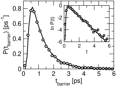
Figure 4: Distribution of permanence times of the proton in the pore after release from the pore center from simulations (circles) and Brownian diffusion on $F(z)$ (solid lines). (Inset: logarithmic scale for $P(t)$.)

The distribution of permanence times of the proton on the free energy barrier can be roughly modeled by a one-dimensional diffusion process on a flat potential, starting from $z=0$ and terminated at $\pm L/2$. The width of the almost flat barrier is $L\approx 8$ Å (Fig. 2). At long times, the resulting distribution of permanence times decays as $P(t)\approx 4\pi D\exp(-\pi^{2}Dt/L^{2})/L^{2}$. This exponential decay accurately reproduces the long time tail of the distribution of permanence times observed in our simulations and plotted in Fig. 4.

The resulting picture of a protonic defect diffusing through the pore under the influence of the effective potential $F(z)$ has implications on the design of conducting pores. Increasing their length $L$ will reduce the transmission coefficient as $1/L$ RUIZ_MONTERO and hence lower the conductance. This effect will be enhanced by the larger desolvation penalty arising in longer pores. However, using nanopores of higher polarity, possibly embedded Bakajin:S:2006 ; Hinds:N:2005 in a high-dielectric medium, should greatly reduce the desolvation cost and may result in the ideal combination of high proton mobility and concentration yielding proton current densities comparable to those measured for polymer electrolyte membranes.

This work was supported by the Austrian Science Fund (FWF) under Grant No. P17178-N02. GH was supported by the Intramural Research Program of the NIH, NIDDK.

References

- (1) K.D. Kreuer, S.J. Paddison, E. Spohr, and M. Schuster, Chem. Rev. 104, 4637 (2004).
- (2) A. Z. Weber and J. Newman, Chem. Rev. 104, 4679 (2004).
- (3) B. Hille, Ion Channels of Excitable Membranes (Sinauer, Sunderland, MA, 2001).
- (4) G. Hummer, J. C. Rasaiah, J. P. Noworyta, Nature 414, 188 (2001); A. Kalra, S. Garde, and G. Hummer, Proc. Natl. Acad. Sci. U.S.A. 100, 10175 (2003).
- (5) R. Pomés and B. Roux, Biophys. J. 75, 33 (1998); Biophys. J. 82, 2304 (2002).
- (6) H. S. Mei, M. E. Tuckerman, D. E. Sagnella, and M. L. Klein, J. Phys. Chem. B 102, 10446 (1998).
- (7) M. L. Brewer, U. W. Schmitt, and G. A. Voth, Biophys. J. 80, 1691 (2001).
- (8) C. Dellago, M. M. Naor, and G. Hummer, Phys. Rev. Lett. 90, 105902 (2003).
- (9) D. J. Mann and M. D. Halls, Phys. Rev. Lett. 90, 195503 (2003).
- (10) S. A. Hassan, G. Hummer, and Y. S. Lee, J. Chem. Phys. 124, 204510 (2006).
- (11) U. W. Schmitt and G. A. Voth, J. Phys. Chem. B 102, 5547 (1998); U. W. Schmitt and G. A. Voth, J. Chem. Phys. 111, 9361 (1999).
- (12) A. Warshel and R. M. Weiss, J. Am. Chem. Soc. 102, 6218 (1980); A. Warshel , “Computer Modeling of Chemical Reactions in Enzymes and Solutions” (Wiley, New York, 1991).
- (13) N. Agmon, Israel J. Chem. 39, 493 (1999).
- (14) H. Lapid, N. Agmon, M. K. Petterson, and G. A. Voth, J. Chem. Phys. 122, 014506 (2005).
- (15) D. Marx, M. E. Tuckerman, J. Hutter, and M. Parrinello, Nature 397, 601 (1999).
- (16) C. Dellago, P. G. Bolhuis, F. S. Csajka, and D. Chandler, J. Chem. Phys. 108, 1964 (1998).
- (17) C. Dellago, P. G. Bolhuis, and P. L. Geissler, Adv. Chem. Phys. 123, 1 (2002).
- (18) T. J. F. Day, A. V. Soudackov, M. Čuma, U. W. Schmitt, and G. A. Voth, J. Chem. Phys. 117, 5839 (2002).
- (19) C. Peter and G. Hummer, Biophys. J. 89, 2222 (2005).
- (20) M. K. Petersen, S. S. Iyengar, T. J. F. Day, and G. A. Voth, J. Phys. Chem. B 108, 14804 (2004).
- (21) C. Radüge, V. Pflumio, and Y. R. Shen, Chem. Phys. Lett. 274, 140 (1997).
- (22) C. H. Bennett, in Algorithms for Chemical Computations, ACS Symposium Series No. 46, edited by R. Christofferson (American Chemical Society, Washington, D.C., 1977).
- (23) D. Chandler, J. Chem. Phys. 68, 2959 (1978).
- (24) C. Dellago and G. Hummer, in preparation (2006).
- (25) R. B. Best and G. Hummer, Proc. Natl. Acad. Sci. USA 102, 6732 (2005).
- (26) G. Hummer, J. Chem. Phys. 120, 516 (2004).
- (27) M. J. Ruiz-Montero, D. Frenkel and J. J. Brey, Mol. Phys. 90, 925 (1997).
- (28) J. K. Holt, H. G. Park, Y. M. Wang, M. Stadermann, A. B. Artyukhin, C. P. Grigoropoulos, A. Noy, and O. Bakajin, Science 312, 1034 (2006).
- (29) M. Majumder, N. Chopra, R. Andrews, and B. J. Hinds, Nature 438, 44 (2005).