Nonlinear response of the magnetophoresis in inverse ferrofluids

Abstract

Taking into account the structural transition and long-range interaction (lattice effect), we resort to the Ewald-Kornfeld formulation and developed Maxwell-Garnett theory for uniaxially anisotropic suspensions to calculate the effective permeability of inverse ferrofluids. And we also consider the effect of volume fraction to the magnetophoretic force on the nonmagnetic spherical particles submerged in ferrofluids in the presence of nonuniform magnetic field. We find that the coupling of ac and dc field case can lead to fundamental and third harmonic response in the effective magnetophoresis and changing the aspect ratio in both prolate and oblate particles can alter the harmonic and nonharmonic response and cause the magnetophoretic force vanish.

I Introduction

Magnetic particles are used to label and manipulate biomaterials such as cells, enzymes, proteins, DNA, to transport therapeutic drugs in the applications such as bioseparation, immunoassays, drug delivery, and to separate red and white blood cells furlani . Magnetizable particles experience a force in a nonuniform magnetic field caused by the magnetic polarization. This phenomenon, called magnetophoresis $(MAP)$ has been exploited in a variety of industrial and commercial process for separation and beneficiation of solids suspended in liquids  1 . Virtually, almost all practical magnetic separation technologies exploit the magnetophoretic forces. Such as, belt and drum devices, high-gradient magnetic separation ($HGMS$) systems Watson etc..

In recent years, inverse ferrofluids with nonmagnetic colloidal particles (or magnetic holes) suspended in ferrofluids have drawn much attention for their potential industrial and biomedical applications  2 ; 3 ; 4 ; 5 . The size of the nonmagnetic particle (such as polystyrene particle) is about 1$\sim$100$\mu$m. Ferrofluids, also know as magnetic fluid, is a colloidal suspension of single-domain magnetic particles, with typical dimension around 10nm, dispersed in a liquid carrier  2 . Because the external magnetic field will induce magnetic dipole moment in the nonmagnetic particles, when the field intensity increases, the inverse ferrofluids will solidify to crystals due to dipole interactions, which is similar to ER and MR behavior. Since the nonmagnetic particles are much larger than the magnetic fluid nanoparticles, the magnetic fluid is treated as a one-component continuum with respect to the larger nonmagnetic particles  7 ; 8 . Recently, Jian, Huang and Tao first theoretically suggested that the ground state of inverse ferrofluids is body-centered tetragonal $(bct)$ lattice  9 , just as the ground states of electrorheological fluids and magnetorheological fluids  10 ; 11 . Motivated by this study, we propose an alternative structural transition from the $bct$ to the face-centered cubic ($fcc$), through the application of external magnetic field. In this work, we will investigate the magnetophoretic force on the particles during the phase transition in the crystal system considering the effects mentioned above.

Finite-frequency responses of nonlinear dielectric composite materials have attracted great attention in both research and industrial applications during the last two decades Bergman . In particular, when a composite containing linear permeability particles embedded in a nonlinear permeability host medium is subjected to a sinusoidal alternating magnetic, the magnetic response will generally consist of frequencies of higher order harmonics under ac field Levy ; Hui ; Huii ; Gu ; Huang ; Wei . The main aim of the present paper is to study the the effects of the geometric shape and volume fraction of the particles on the nonlinear ac responses (harmonics) of the crystal system, then the magnetophoresis of the particles, considering the local lattice effect. We shall use the Edward-Kornfeld formulation 12 ; 13 ; 14 to derive the local magnetic fields and induced dipole moments in inverse ferrofluids and then perform the perturbation expansion method to obtain the fundamental and higher harmonics in two cases: single ac and dc-ac magnetic field.

Then, we apply a nonuniform magnetic field to investigate the magnetophoresis of the nonmagnetic particles submerged in the ferrofluids, by taking into account the effect of structural transition and long-range interaction (lattice effect). And we also consider the effect of volume fraction to the magnetophoretic force exerted on the nonmagnetic particles.

This paper is organized as follows. In Sec. II, we introduce the nonlinear characteristics in the ferrofluids and the theory of magnetophoresis. By using the Ewald-Kornfeld formulation and the well-known developed Maxwell-Garnett theory for uniaxially anisotropic suspensions, we calculate the effective permeability of the inverse ferrofluids for different harmonic response under time-varying magnetic field in Sec. III. Then we investigate the nonlinear response of magnetophoretic force on the nonmagnetic particles in ferrofluids. This paper ends with a discussion and conclusion in Sec. IV.

II Theory and Formalism

II.1 Nonlinear characteristics in the ferrofluids

In the standard literature, we often consider the magnetic induction B to be proportional with the field strength $\textbf{H}_{0}$, and their relation is written as $\textbf{B}=\mu\textbf{H}_{0}$, where $\mu$ is the linear permeability. However, the simple relation is only valid at weak intensities. When in the real situation, especially under a stronger field, nonlinearities are introduced as $\textbf{B}=\mu\textbf{H}_{0}+\xi|H_{0}|^{2}\textbf{H}_{0}+\eta|H_{0}|^{4}\textbf{H}_{0}+...$, where $\xi$,$\eta$ are the third-order and fifth-order nonlinear coefficient and $\eta|H_{0}|^{4}\ll\xi|H_{0}|^{2}\ll\mu$. Here we assume the nonlinearity is not strong and consider only the lowest-order nonlinearity for simplicity. Thus after dropping the symbol of absolute value in the equation above, the nonlinear permeability $\tilde{\mu}$ is obtained:

$$\tilde{\mu}=\mu_{1}+\xi_{1}H_{0}^{2}$$ (1)

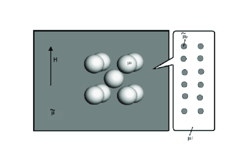
Figure 1: Jian, Gao, and Huang

For inverse ferrofluids, the peameability $\tilde{\mu}$ of host medium ferrofluid can be derived in the form as $\tilde{\mu}=\mu_{1}+\xi_{1}H_{0}^{2}$ when the magnetic particles in the ferrofluid is nonlinear to the external field, as analyzed below. As shown in Fig.(1), considering the magnetic particles with nonlinear $\tilde{\mu}_{p}$ in the ferrofluid , the local magnetic field $\textbf{H}_{1}$ inside the particle induced by external field $\textbf{H}_{0}$ is give by

$$\textbf{H}_{1}=\frac{3\mu_{f}}{\tilde{\mu}_{p}+2\mu_{f}}\textbf{H}_{0}$$ (2)

Here $\mu_{f}$ represents the host medium permeability in the ferrofluid, and the nonlinear permeability $\mu_{p}$ of the magnetic particle can be expressed as $\tilde{\mu}_{p}=\mu_{p}+\xi H_{1}^{2}$ with $\xi$ being the nonlinear coefficient. For the spherical shape particles, the effective permeability $\mu_{f,e}$ of the whole ferrofluid can be determined by the Maxwell-Garnett theory 18

$$\frac{\mu_{f,e}-\mu_{f}}{\mu_{f,e}+2\mu_{f}}=f\frac{\tilde{\mu}_{p}-\mu_{f}}{\tilde{\mu}_{p}+2\mu_{f}}$$ (3)

where $f$ denotes the volume fraction of the magnetic particles in ferrofluid. Applying Eq.(2) and (3) and performing the Taylor expansion by taking $\xi H_{1}^{2}$ as a small perturbation, we can obtain

$$\mu_{f,e}=\frac{\mu_{f}[(1+2f)\mu_{p}-2(f-1)\mu_{f}]}{(1-f)\mu_{p}+(2+f)\mu_{f}}+\frac{81f\mu_{f}^{4}\xi H_{0}^{2}}{[(1-f)\mu_{p}+(2+f)\mu_{f}](\mu_{p}+2\mu_{f})^{2}}+O[\xi^{2}]$$ (4)

Hence the nonlinear permeability of ferrofluid can be expressed as

$$\tilde{\mu}=\mu_{f,e}=\mu_{1}+\xi_{1}H_{0}^{2}$$ (5)

in which the constants $\mu_{1}=\frac{\mu_{f}[(1+2f)\mu_{p}-2(f-1)\mu_{f}]}{(1-f)\mu_{p}+(2+f)\mu_{f}},\xi_{1}=\frac{81f\mu_{f}^{4}\xi}{[(1-f)\mu_{p}+(2+f)\mu_{f}](\mu_{p}+2\mu_{f})^{2}}+O[\xi^{2}]$ We emphasize that when the magnetic particles form chains under strong external field, Eq. (3) is supposed to modify by introducing demagnetization factor 20 , but the expression of $\tilde{\mu}$ will remain unchanged by appropriately choosing $\mu_{1}$ and $\xi_{1}$.

II.2 Local Magnetic Field and Induced Dipole Moment

When the inverse ferrofluids system forms crystal under external field, there are two dominant factors effecting its effective permeability: the local field of crystal structure and the geometrical shape of the particles which makes up of the crystal. Below we will first investigate the local field factor by performing an Ewald-Kornfeld formulation so that the structural transition and long-range interaction can be taken into account explicitly. Considering the ground state of inverse ferrofluids as a body-centered-tetragonal ($bct$) lattice, which can be regarded as a tetragonal lattice, plus a basis of two particles each of which is fixed with an induced point magnetic dipole at its center. One of the two particles is located at a corner and the other one at the body center of the tetragonal unit cell, as shown in Fig.(1). Its lattice constants are denoted by $a(=b)=\xi q^{-\frac{1}{2}}$ and $c$= $\xi q$ along $x(y)$ and $z$ axes. In this case we identified a different structure transformation from the $bct$ to $fcc$ to $bcc$ by changing the uniaxial lattice constant $c$ under hard-sphere constraint. As $q$ varies the volume of unit cell remains $v_{c}=\xi^{3}$ . In this way, the degree of anisotropy of tetragonal lattice is measured by how $q$ is deviated from unity and the uniaxial anisotropic axis is along the $z$ axis. In particular, $q=0.87358$, 1 and $2^{\frac{1}{3}}$ represent the $bct$, $bcc$ and $fcc$ lattice, respectively.

In case of an external magnetic field $H_{0}$ along the $z$ axis, the induced dipole moment $\overrightarrow{\textbf{m}}$ are perpendicular to the uniaxial anisotropic axis. The local field $H_{L}$ at the lattice point $\vec{R}$=0 can be determined by using the Ewald-Kornfeld formulation  12 ; 13 ; 14 ,

$$H_{L}=\textbf{m}\cdot\sum_{j=1}^{2}\sum_{\vec{R}\neq\vec{0}}[-\gamma_{1}(R_{j})+x_{j}^{2}q^{2}\gamma_{2}(R_{j})]-\frac{4\pi\textbf{m}}{v_{c}}\sum_{\vec{G}\neq\vec{0}}\Pi(\vec{G})\frac{G_{x}^{2}}{G^{2}}\exp\left(\frac{-G^{2}}{4\eta^{2}}\right)+\frac{4\textbf{m}\eta^{3}}{3\sqrt{\pi}}$$ (6)

In this equation, $\gamma_{1}$ and $\gamma_{2}$ are two coefficients, given by,

$$\gamma_{1}(r)=\frac{\rm erfc(\eta r)}{r^{3}}+\frac{2\eta}{\sqrt{\pi}r^{2}}\exp(-\eta^{2}r^{2})$$ (7)

$$\gamma_{2}(r)=\frac{3\rm erfc(\eta r)}{r^{5}}+(\frac{4\eta^{3}}{\sqrt{\pi}r^{2}}+\frac{6\eta}{\sqrt{\pi}r^{4}})\exp(-\eta^{2}r^{2})$$ (8)

where erfc$(\eta r)$ is the complementary error function, and $\eta$ is an adjustable parameter making the summations in real and reciprocal lattices converge rapidly. In Eq. (7), $R$ and $G$ denote the lattice vector and reciprocal lattice vector, respectively,

$$\vec{R}=\xi(q^{-\frac{1}{2}}l\hat{x}+q^{-\frac{1}{2}}m\hat{y}+qn\hat{z})$$ (9)

$$\vec{G}=\frac{2\pi}{\xi}(q^{\frac{1}{2}}u\hat{x}+q^{\frac{1}{2}}v\hat{y}+q^{-1}w\hat{z})$$ (10)

where, $l,m,n,u,v,w$ are integers. In addition, $z_{j}$ and $R_{j}$ are respectively given by,

$$z_{j}=l-\frac{j-1}{2},R_{j}=|\vec{R}-\frac{j-1}{2}(a\hat{x}+a\hat{y}+c\hat{z})|$$ (11)

and $\Pi(\vec{G})=1+\exp[i(u+v+w)/\pi]$ is the structure factor. The local field will be computed by summing over all integer indices $(j,l,m,n)\neq(1,0,0,0)$ for the summation in real lattice and $(u,v,w)\neq(0,0,0)$ for the summation in the reciprocal lattice. Here we consider an infinite lattice. For finite lattices, one must be careful about the effects of different boundary conditions  15 . Because of the exponential factors, we may impose an upper limit to the indices, i.e., all induces ranging from $-L$ to $L$, where $L$ is a positive integer.

Now, let us define a local field factor $\alpha$,

$$\alpha=\frac{3v_{c}}{4\pi}\frac{H_{L}}{\textbf{m}}$$ (12)

It is worth noticing that $\alpha$ is a function of single variable $q$. Also, there is a sum rule 2$\alpha_{\perp}$ +$\alpha_{\parallel}$ =3  16 ; 17 , where $\alpha_{\parallel}$ denotes the local field factor in longitudinal field case, while $\alpha_{\perp}$ denotes the local field in transverse case. Here the longitudinal (or transverse) field case corresponds to the fact the $H_{0}$ field is parallel (or perpendicular) to the uniaxial anisotropic $z$ axis.

II.3 Nonlinear AC response in the Cases of Spheroids

Now we are in the position to take into the account the geometrical shape effect of the particles by investigating nonspheres: prolate and oblate. In MR(ER or inverse ferrofluids) fluid, the shear stress and permeability(permittivity) will be enhanced by changing the ratio of the ellipsoidal particles in the chain  Shaw such as $p$-phenylene-2, 6- benzobisthiazole polyparticle. This induced polarization can be described in demagnetizing factor, which includes the three principal axes of the spheroid. For a prolate spheroid($a=b<c$), the longitudinal demagnetizing factor $g_{l}$ along the major axis $c$ is given by $g_{l}=\frac{k\rm ln(k+\sqrt{k^{2}-1})}{(k^{2}-1)^{\frac{3}{2}}}-\frac{1}{k^{2}-1}$ with $k=\frac{c}{a}$; for oblate case($a<b=c$), $g_{l}=1-\frac{k^{2}\rm arcsin\frac{\sqrt{k^{2}-1}}{k}}{(k^{2}-1)^{\frac{3}{2}}}+\frac{1}{k^{2}-1}$. There is a sum rule for the longitude and transverse demagnetizing factor 18 ; 20 that $g_{l}+2g_{t}=1$. For prolate spheroid, because it can easily align with its major axis($c$) along the direction of the external field, while the dipole moments of nonmagnetic particles are oriented opposing the external field, here we only focus on the longitude case. It is also worth noticing that the spherical shape of particles is included when $g_{l}=g_{t}=\frac{1}{3}$.

Now We can use the developed Maxwell-Garnett theory for uniaxially anisotropic suspensions  18 ; 19 considering both the local lattice and geometrical shape effect to derive the effective permeability 20

$$\frac{\frac{1}{3}\alpha(\mu_{e}-\tilde{\mu})}{\tilde{\mu}+\frac{1}{3}\alpha(\mu_{e}-\tilde{\mu})}=p\frac{g_{l}(\mu_{0}-\tilde{\mu})}{\tilde{\mu}+g_{l}(\mu_{0}-\tilde{\mu})}$$ (13)

Similar to the technique applying in Eq.(4), combining Eq.(1) we admit

$$\mu_{e}=\frac{\mu_{1}[\alpha\mu_{1}+g_{l}(x\alpha-3p)y]}{\alpha[(\mu_{1}+g_{l}xy]}+\xi H_{0}^{2}\frac{\alpha\mu_{1}^{2}+g_{l}^{2}xy^{2}[x\alpha-3p]+2\alpha g_{l}\mu_{1}xy}{\alpha[yg_{l}-\mu_{1}]^{2}[\mu_{1}+g_{l}xy]^{2}}+\frac{3g_{l}^{2}\mu_{0}^{2}\mu_{1}^{4}px\xi^{2}H_{0}^{4}}{\alpha[\mu_{1}-g_{l}y]^{4}[\mu_{1}+g_{l}xy]^{3}}+O[\xi^{3}]$$ (14)

with $x=p-1,y=\mu_{1}-\mu_{0}$.

In the presence of external oscillating time-varying magnetic field cite21 , the magnetic particles will have nonlinear characteristics and the inverse ferrofluids system will induce harmonic response at different frequencies without phase transition 10 . In the experiment, the second term or higher order terms on the right-hand of Eq. (14) can be obtained using mixed-frequency measurements yang . In this paper, we will focus on the characteristics of the harmonics of effective permeability for the inverse ferrofluid and their nature on the magnetophoresis when particles put in: $\mu_{0},\mu_{\omega},\mu_{2\omega}...$. In case of an external sinusoidal magnetic field(ac) of the form

$$H_{0}=H_{ac}\rm sin\omega t$$ (15)

Applying Eq.(15) into Eq.(14), we can obtain zero, second and fourth order harmonics for the effective permeability: $\mu_{e}=\mu_{0}+\mu_{2\omega}\rm cos2\omega t+\mu_{4\omega}\rm cos4\omega t$. Here we give the expression for $\mu_{4\omega}$:

$$\mu_{4\omega}=\xi H_{ac}^{2}\frac{3g_{l}^{2}\mu^{4}px}{8\alpha[g_{l}xy+\mu]^{3}[\mu-g_{l}y]^{4}}$$ (16)

On the other hand, under the application of a dc and ac field, namely,

$$H_{0}=H_{dc}+H_{ac}\rm sin\omega t$$ (17)

Using the same technique we can rewrite the effective permeability as $\mu_{e}=\mu_{0}+\mu_{\omega}\rm sin\omega t+\mu_{2\omega}\rm cos2\omega t+\mu_{3\omega}\rm sin3\omega t+\mu_{4\omega}\rm cos4\omega t$, for extracting different harmonics.

II.4 Magnetophoresis in inverse ferrofluids system

Now we will investigate the magnetophoretic behavior when particles are put in inverse ferrofluids. In a standard case, a magnetically polarizable object will be trapped in a region of a focused magnetic field, or nonmagnetic particles in a magnetizable liquid(ferrofluid), provided there is sufficient magnetic response to overcome thermal energy and the magnetophoretic force 1 . Here we consider the nonmagnetically homogenous particle in the nonlinear inverse ferrofluids for simplicity, and the magnetic field is assumed to be $dc$ and hysteresis is ignored. For a magnetically linear particle under magnetophoresis, the effective magnetic dipole moment vector induced inside takes a form very similar to that for the effective dipole moment of dielectric paricle 2 ; chou , $\vec{m}=4\pi R_{eff}^{3}b\vec{H}_{0}$, where $R_{eff}$ is the effective radius of spherical or spheroidal particle and $b$ is the clausius-Mossotti factor(CMF) along the direction of external field. Here we focus on the magnetophoresis of spherical particle in inverse ferrofluids, and CMF $b$ is written as: $b=\frac{\mu_{2}-\mu_{e}}{\mu_{2}+2\mu_{e}}$ where $\mu_{2}$ is the permeability of nonmagnetic particle, and $\mu_{e}$ is the permeability of the host medium: inverse ferrofluids. It should be noted, that in a general case, for spheroidal particle, CMF $b$ is written as $\frac{1}{3}\frac{\mu_{2}-\mu_{e}}{\mu_{e}+g_{l}(\mu_{2}-\mu_{e})}$. The force exerted by a nonuniform magnetic field on the dipole can be obtained:

$$\vec{F}_{{dipole}}=\mu_{e}\vec{m}\cdot\nabla H_{0}$$ (18)

Combining the effective magnetic dipole moment, the magnetophoretic force exerted on the spherical particle in a nonuniform magnetic field can be written as,

$$\vec{F}_{MAP}=2\pi\mu_{e}R^{3}b\nabla H_{0}^{2}$$ (19)

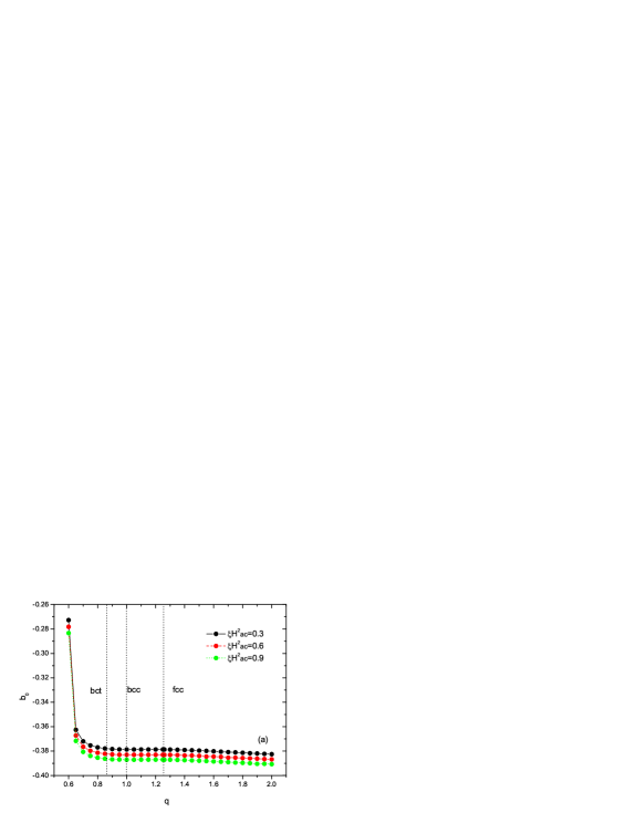
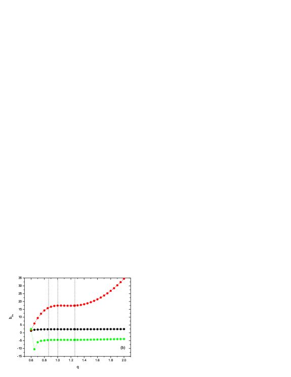
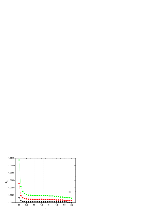
Figure 2: Jian, Gao, and Huang

Thus the magnetophoretic force on particles are proportional to the particle volume, the polarization difference and distribution of the geometric field gradient. There are two kinds of magnetophoresis depended upon the relative magnitudes of $\mu_{2}$ and $\mu_{e}$. Particles are attracted to magnetic field intensity maxima and repelled to the field-generating electrodes when $b>0$ as positive magnetophoresis and negative magnetophoresis corresponds to $b<0$. Based on the harmonics of effective permeability, the expressions for the CMF can explicitly be obtained when the lattice structure of the host medium is changed, as shown in Fig. 2. The degree of anisotropy $q$ plays an important role in determining the local field factor $\alpha$. There is a plateau during the structure transformation on the relationship between $q$ and $\alpha$ Huang , accordingly we can also predict similar behavior in CMF, especially in Fig. 2(b). It is found that increasing $q$ causes both zero and fourth order harmonic CMF decreases in Fig. 2(a) and Fig. 2(c). Note that when $q$ changes from 0.6 to 0.8 all CMF have great decreasing and CMF in Fig. 2(c) changes its sign when the nonlinearity is the highest, thus demonstrating the sensitivity of CMF when the system is under structure changes. Although the fourth-order harmonics of the local magnetic field and induced dipole moment seems to be complicated, since the strength of the nonlinear polarization of nonlinear materials can be reflected in the magnitude of the high-order harmonics of local magnetic field and dipole moment, the effective nonlinear part in the effective nonlinear magnetic constant can be expected to determine the magnitude of the fourth-order harmonics.

III Numerical Results

In the preceding section we will calculate the effect of spheroidal shape and volume fraction of nonmagnetic particles which forms bct lattice structure in the ferrofluids, on the harmonic response of CMF. For a special case, when we would like to conclude the nonharmonic response situation, the external field $H_{0}$ is constant and not vary with time namely, it can be easily obtained without tedious calculation by setting $\omega t=\frac{\pi}{2}$ for ac field in Eq. (15). Thus only the zero harmonic contributes. Similar conclusions can be obtained that only $b_{0}+b_{\omega}-b_{3\omega}$ contributes in a dc and ac field case.

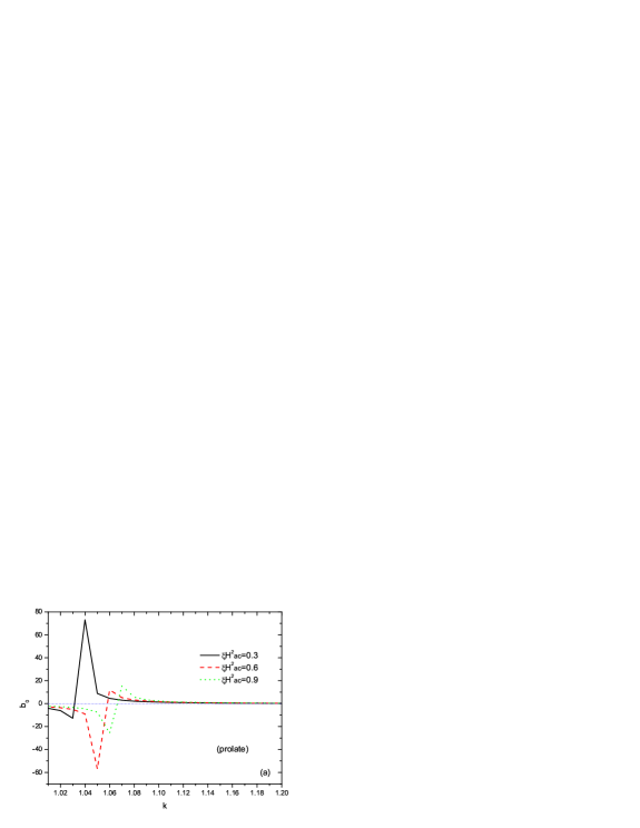
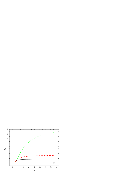
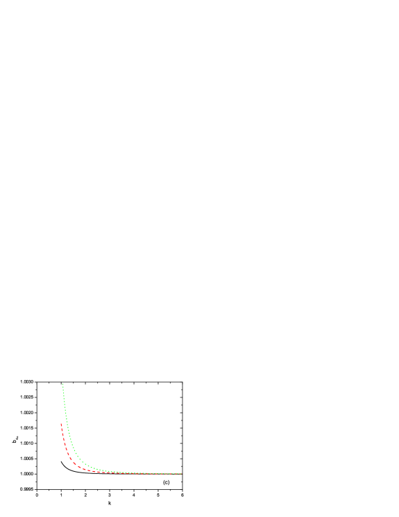
Figure 3: Jian, Gao, and Huang

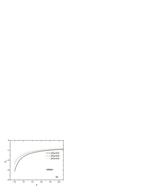
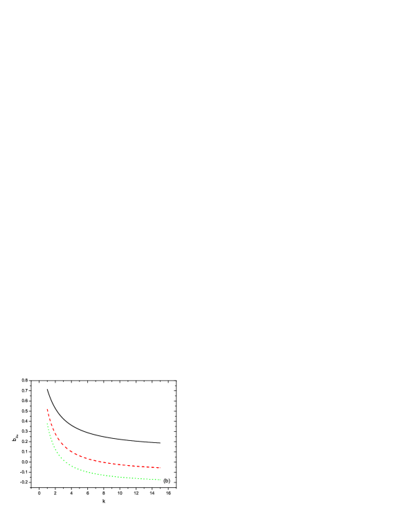
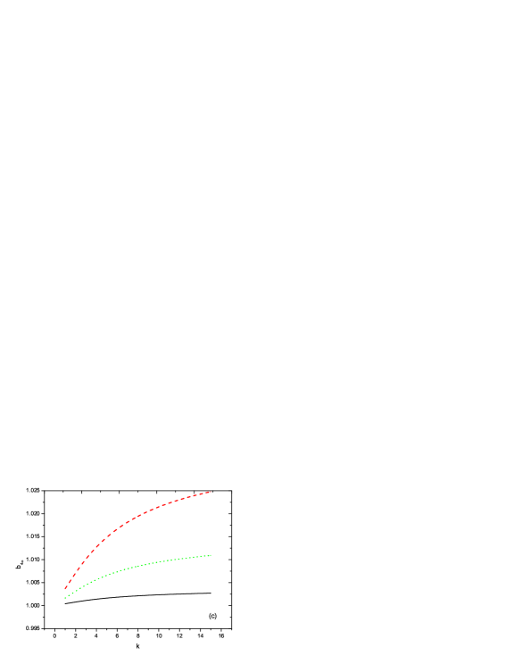
Figure 4: Jian, Gao, and Huang

In Fig. 3 and Fig. 4 we show the harmonic response of CMF for different shapes in ac field: prolate and oblate. The zero(or nonharmonic) response of CMF exhibits strong sensitivity to the prolate demagnetization factor(the shape) and some peaks are obtained, while for oblate CMF $b_{0}$ have slight change compared(Fig. 4). This can be briefly explained through self-consistent approach 22 by the spectral representation separating the material parameter $s=(1-\mu_{0}/\mu)$ from the geometrical parameters. Without considering the crystal lattice effect, the effective permeability can be derived as $\mu_{e}=\mu[1-\frac{p}{s-g_{l}(1-p)}]$. It is clear that decreasing $g_{l}$ leads to increasing $\mu_{e}$, while for prolate(oblate) case, increasing aspect ratio $k$ causes increasing(decreasing) of $g_{l}$. In the meantime, because of the existence of weak nonlinearity, the nonlinear polarization has just a perturbation effect, which can be neglected when compared to the linear part. Furthermore, we can predict that one or two shape-dominant crossover ratio at which there is no net force on the particle in the magnetophoresis. In Fig. 3(a), it is interesting that the crossover ratio is monotonically increasing as the nonlinearity increases. Fig. 4 shows that, as nonlinear characteristics increase, the harmonics response of CMF are caused to increase accordingly for oblate particles. We emphasize to point out that, although prolate and oblate particles can both exist in different system state, the alignment of one particle can only be along the longest axis(prolate) when the particle is homogenous under the external magnetic field.

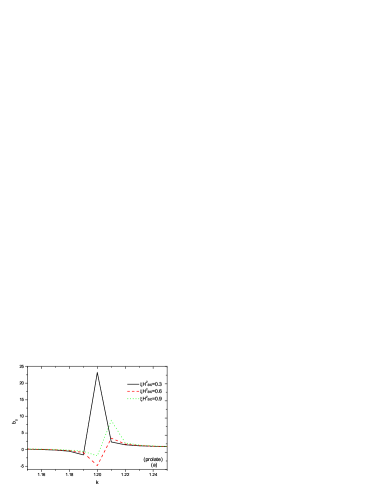
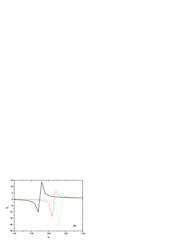
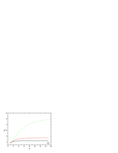
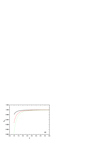
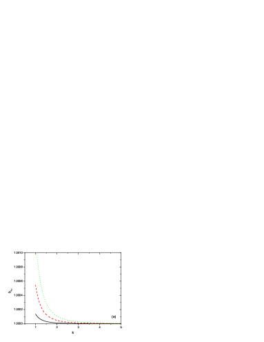
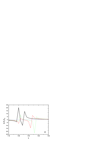
Figure 5: Jian, Gao, and Huang

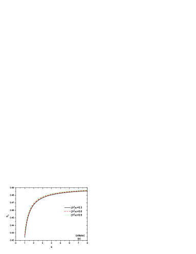
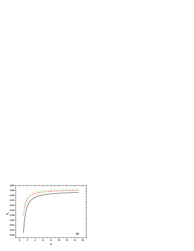
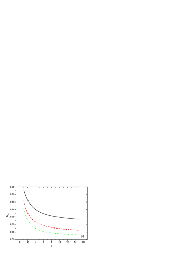
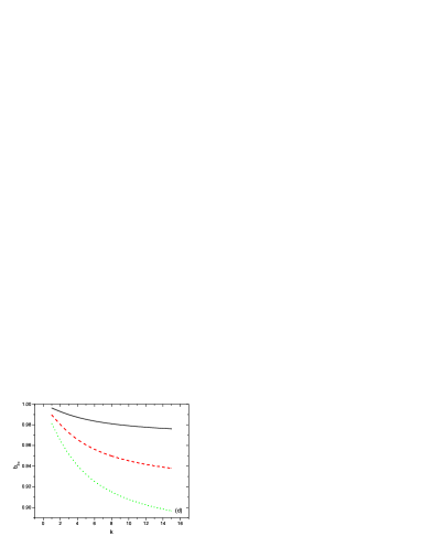
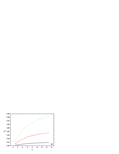
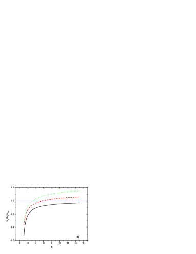
Figure 6: Jian, Gao, and Huang

Fig. 5 and Fig. 6(a)-(e) show different harmonic response of CMF for prolate and oblate particle in dc and ac field. Comparing with in single ac field, the response nature of CMF keeps unchanged for the same harmonics. So the introduction of coupling between dc and ac field add more odd harmonic response. As discussed above the nonharmonic response of CMF can be obtained as $b_{0}+b_{\omega}-b_{3\omega}$, which is shown in Fig. 5(f) and Fig. 6(f).It is also found that lower harmonic response of CMF can be several orders of magnitude larger than the higher one.

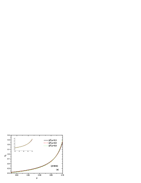
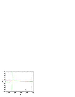
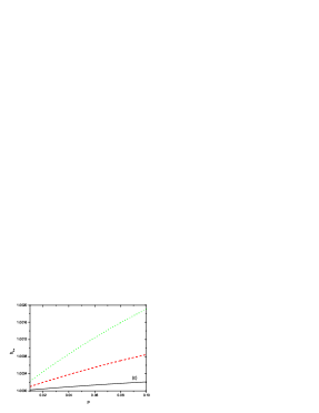
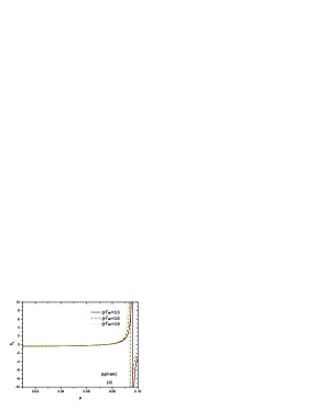
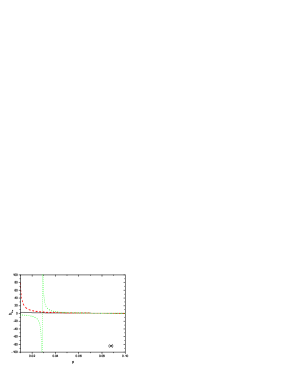
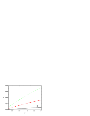
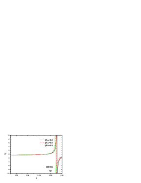
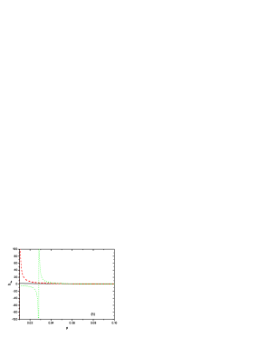
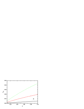
Figure 7: Jian, Gao, and Huang

Fig. 7 displays for prolate, oblate spheroidal and spherical particle, the effect of volume fraction of magnetic particles in the ferrofluids on the harmonic response of CMF. It is observed from Fig. 7(a) that the nonlinearity for nonharmonic response has little effect on CMF. The reason is that in the system of interest only ferrofluids are assumed to be nonlinear while the particles are linear. As the volume fraction of particles increases, the nonlinear component within the system have slight change naturally, yielding unchanged CMF accordingly. The second and fourth order response of CMF in Fig. 7(b) and (c) shows great variety when the volume fraction changes. This enhancement of the harmonics may arise from the mutual interaction between the dipole moments: when increasing the volume fraction, the mutual interaction becomes strong and leads to shift of harmonic response. It is observed that for prolate particles, the nature of zero-order response of CMF is greatly different from that of oblate spheroidal and spherical particles, comparing Fig. 7(a) with Fig. 7(d) and Fig. 7(g).

IV Discussion and Conclusion

In this work, we have investigated both the effect of lattice structure of crystal and the geometrical shape of particles embedded in the ferrofluids on the nonlinear response of magnetophoresis using the perturbation method. The nonlinear response of CMF under the structure transition is studied in detail. It is thus possible to perform a real-time monitoring of structure transformation. We find that the coupling of ac and dc field case can lead to fundamental and third harmonic response in the effective permeability constant and the CMF respectively. We also find that change the aspect ratio in both prolate and oblate particles can alter the harmonic and nonharmonic response and thereby causing the magnetophoretic force vanish. Furthermore, by taking into account the local-field effect from the mutual interaction, we examine the CMF response in various volume fractions, and find that increasing volume fraction can result in the enhancement of the strengths and the difference between the different nonlinearities and characteristic harmonics. Thus, it is possible to obtain a good agreement between theoretical predictions and experimental data by suitable adjustment of both the geometric parameters(for example, the particle shape) and the physical parameters(for example, the temperature, component ratio in the system, saturation magnetization, initial magnetic susceptibility). On the contrary, such fitting is useful to obtain the relevant physical information of magnetophoresis in inverse ferrofluid.

We demonstate theoretically the shape effect of the effective magnetic constant in the inverse ferrofluids system. It is in fact that the magnetic particles in the ferrofluid are inhomogeneous in the real case. A first-principle study of the dielectric dispersion of inhomogeneous suspension is presented Huang ; norina , and can be used to analyze the magnetic dispersion in the dilute limit, in which the permeability of the ferrofluid is dependent on the frequencies of external magnetic field. Also when the inhomogeneity is simplified as the shelled spheroidal particles in the ferrofluid system Bizdoaca , a self-consistent method 23 can be applied for the three-component composites. The magnetic anisotropy as well as geometric anisotropy can both be taken into account, and will be reported elsewhere.

The nonlinearity under our consideration is weak, which is common in real situations under moderate fields, while in case of strong nonlinearity, the perturbation approach is no longer valid and should be adopted using self-consistent method instead 24 . And in the above discussion, we consider the longitude case under the external field, it can also be found constricted by the relation $g_{l}+2g_{t}=1$, the harmonic response of CMF have opposite behavior.

Figure Captions

Fig.1. (Color online) Schematic graph showing the inverse ferrofluid system, in which the crystal consisted of nonmagnetic particles(permeability is denoted by $\mu_{0}$) embed in the ferrofluid($\tilde{\mu}_{0}$). Ferrofluids contain nanosize ferromagnetic particles($\tilde{\mu}_{p}$) dispersed in a carrier fluid($\mu_{f}$).

Fig.2. (Color online) The zero, second, fourth harmonic response of CMF versus degree of anisotropy $q$ for different intrinsic nonlinear characteristics in the prolate case. The bct, bcc and fcc lattices which are respectively related to $q=0.87358,1.0,2^{\frac{1}{3}}$ are shown(dot lines). Parameters: $\mu_{0}=\mu_{2}=1,\mu_{1}=2,p=0.1,k=1.2$.

Fig.3. (Color online) Cases of prolate spheroidal particles: ac field. Zero, second, fourth harmonic response of CMF versus $k=c/a$ for different intrinsic nonlinear characteristics. Parameters: $\mu_{0}=\mu_{2}=1,\mu_{1}=2,p=0.1,\alpha=0.95351$.

Fig.4. (Color online) Cases of oblate spheroidal particles: ac field. Zero, second, fourth harmonic response of CMF versus $k=c/a$ for different intrinsic nonlinear characteristics. Parameters: $\mu_{0}=\mu_{2}=1,\mu_{1}=2,p=0.1,\alpha=0.95351$.

Fig.5. (Color online) Cases of prolate spheroidal particles: ac and dc field. Zero, fundamental, second, third, fourth harmonic response of CMF versus $k=c/a$ for different intrinsic nonlinear characteristics (a)-(e). Parameters: $\mu_{0}=\mu_{2}=1,\mu_{1}=2,p=0.1,\alpha=0.1,H_{dc}=\sqrt{3.6}$. (f) show the nonharmonic response of CMF.

Fig.6. (Color online) Cases of oblate spheroidal particles: ac and dc field. Zero, fundamental, second, third, fourth harmonic response of CMF versus $k=c/a$ for different intrinsic nonlinear characteristics (a)-(e). Parameters: $\mu_{0}=\mu_{2}=1,\mu_{1}=2,p=0.1,\alpha=0.95351,H_{dc}=\sqrt{3.6}$. (f) show the nonharmonic response of CMF.

Fig.7. (Color online) Zero, second, fourth harmonic response of CMF versus volume fraction $p$ for different intrinsic nonlinear characteristics in cases of prolate((a)-(c)), oblate((g)-(i)) spheroidal particles and spherical particles((d)-(f)) under ac field. Parameters: $\mu_{0}=\mu_{2}=1,\mu_{1}=2,k=1.2,\alpha=0.95351$.

.

References

- (1) E. P. Furlani, Jour. Appl. Phys. 99, 024912 (2006); Pulak Natha, Lee R. Moore, Maciej Zborowski, Shuvo Roy and Aaron Fleischman, Jour. Appl. Phys. 99, 08R905 (2006); Ki-Ho Han and A. Bruno Fraziera, Jour. Appl. Phys. 96, 5797 (2004)
- (2) T. B. Jones, Electromechanics of Particles (Cambridge University Press, Cambridge, 1995), Chap.III.
- (3) J. H. P. Watson, J. Appl. Phys. 44, 4209 (1973).
- (4) A. T. Skjeltorp, Phys. Rev. Lett, 51, 2306 (1983); R. R. Birss, R. Gerber, and M. R. Parker, IEEE Trans. Magn. MAG-12, 892 (1976).
- (5) J. Ugelstad et al, Blood Purif. 11, 349 (1993)
- (6) J. B. Hayter, R. Pynn, S. Charles, A. T. Skjeltorp, J. Trewhella, G. Stubbs, and P. Timmins, Phys. Rev. Lett. 62, 1667 (1989)
- (7) A. Koenig, P. H ebraud, C. Gosse, R. Dreyfus, J. Baudry, E. Bertrand, and J. Bibette, Phys. Rev. Lett. 95, 128301 (2005)
- (8) Efraim Feinstein and Mara Prentiss, J. Appl. Phys. 99, 064910 (2006)
- (9) B. J. de Gans, C. Blom, A. P. Philipse, and J. Mellema, Phys. Rev. E. 60, 4518 (1999)
- (10) Y. C. Jian, J. P. Huang and R. Tao, Structure of polydisperse inverese ferrofluids: Theory and computer simulation, (to be published).
- (11) R. Tao and J. M. Sun, Phys. Rev. Lett. 67, 398 (1991); R. Tao and Q. Jiang, Phys. Rev. Lett. 73, 205 (1994)
- (12) Lei Zhou, Weijia Wen, and Ping Sheng, Phys. Rev. Lett. 81, 1509 (1998)
- (13) Chin-Yih Hong, C. C. Wu, Y. C. Chiu, S. Y. Yang, H. E. Hornga, and H. C. Yang, Appl. Phys. Lett. 88, 212512 (2006)
- (14) J. P. Huang, Phys. Rev. E 70, 041403 (2004)
- (15) P. P. Ewald, Ann. Phys. (Leipzig) 64, 253 (1921); H. Kornfeld, Z. Phys. 22, 27 (1924)
- (16) C. F. Chou, J. O. Tegenfeldt, O. Bakajin, S. S. Chan, E. C. Cox, N. Darnton, T. Duke, and R. H. Austin, Biophys. Jour. 83, 2170 (2002)
- (17) C. L. Asbury and Ger van den Engh, Biophys. Jour. 74, 1024 (1998)
- (18) J. P. Huang and K. W. Yu, Appl. Phys. Lett. 87, 071103 (2005).
- (19) M. Allen and D. Tildesley, Computer Simulation of Liquids (Oxford Science, London, 1990)
- (20) C.K. Lo and K.W. Yu, Phys. Rev. E 64, 031501 (2001)
- (21) L. D. Landau, E. M. Lifshitz, and L. P. Pitaevskii, Electrodynamics of Continuous Media, 2nd ed. (Pergamon, New York, 1984), Chap. II.
- (22) J. C. M. Garnett, Philos. Trans. R. Soc. London, Ser. A 203,385 (1904); 205, 237 (1906). C. J. F. Böttcher, Theory of Electric Polarization. 2nd ed.(Elsevier, Amsterdam), Vol 1 (1993)
- (23) D. J. Bergman and D. Stroud, Solid State Phys. 46, 146 (1992)
- (24) O. Levy, D. J. Bergman and D. Stroud, Phys. Rev. E. 52, 3184 (1995)
- (25) P. M. Hui and D. Stroud, J. Appl. Phys. 82, 4740 (1997)
- (26) P. M. Hui, P. C. Cheung and D. J. Stoud, J. Appl. Phys. 84, 3451 (1998)
- (27) G. Q. Gu, P. M. Hui and K. W. Yu, Physica B. 279, 62 (2000)
- (28) R. C. Kanu and M. T. Shaw, Inter. Jour. Mod. Phys. B. 10, 2925 (1996); R. C. Kanu and M. T. Shaw, J. Rheol. 42, 657 (1998)
- (29) J. P. Huang, L. Gao and K. W. Yu, J. Appl. Phys. 93, 2871 (2003); J. P. Huang, J. Phys. Chem. B 109, 4824 (2005); G. Wang, W. J. Tian and J. P. Huang, J. Phys. Chem. B 110, 10738 (2006); J. Lei, Jones T. K. Wan, K. W. Yu, and H. Sun, Phys. Rev. E. 64, 012903 (2001)
- (30) E. B. Wei, J. B. Song and G. Q. Gu, J. Appl. Phys. 95, 1377 (2004)
- (31) J. P. Huang, J. T. K. Wan, C. K. Lo, and K. W. Yu, Phys. Rev. E 64, 061505 (2001)
- (32) J. P. Huang and K. W. Yu, Phys. Rep. 431, 87 (2006); C. Z. Fan and J. P. Huang, Appl. Phys. Lett. 89, 1 (2006)
- (33) D. J. Bergman, Phys. Rep. 43, 377 (1978)
- (34) S. B. Norina, Proc. SPIE-OSA Biom. Opt. 5143, 126 (2003)
- (35) E. L. Bizdoaca, M. Spasova, M. Farle, M. Hilgendorff, L. M. Liz-Marzan and F. Carusob, J. Vac. Sci. Technol. A 21(4), 1515 (2003)
- (36) L. Gao, Jones T. K. Wan, K. W. Yu, and Z. Y. Li, J. Phys.: Condens. Matter. 12, 6825 (2000)
- (37) J. T. K. Wan, G. Q. Gu and K. W. Yu, Phys. Rev. E. 63, 052501 (2001)