Heat conduction through a trapped solid: effect of structural changes on thermal conductance

Abstract

We study the conduction of heat across a narrow solid strip trapped by an external potential and in contact with its own liquid. Structural changes, consisting of addition and deletion of crystal layers in the trapped solid, are produced by altering the depth of the confining potential. Nonequilibrium molecular dynamics simulations and, wherever possible, simple analytical calculations are used to obtain the thermal resistance in the liquid, solid and interfacial regions (Kapitza or contact resistance). We show that these layering transitions are accompanied by sharp jumps in the contact thermal resistance. Dislocations, if present, are shown to increase the thermal resistance of the strip drastically.

1 Introduction

The transport of heat through small and low dimensional systems has enormous significance in the context of designing useful nano-structures [1]. Recently, it was shown[2] that a narrow solid strip trapped by an external potential[3, 4, 5, 6] and surrounded by its own fluid relieves mechanical stress via the ejection or absorption of single solid layers[7, 8, 9] to and from the fluid. The trapping potential introduces large energy barriers for interfacial capillary fluctuations thereby forcing the solid-liquid interfaces on either side of the solid region to remain flat. The small size of the solid also inhibits the creation of defects since the associated inhomogeneous elastic displacement fields need to relax to zero quickly at the boundaries, making the elastic energy cost for producing equilibrium defects prohibitively large. Therefore the only energetically favourable fluctuations are those that involve transfer of complete layers which cause at most a homogeneous strain in the solid[2]. Such layering transitions were shown to affect the sound absorption properties of the trapped solid in rather interesting ways[2]. What effect, if any, do such layering transitions have for the transfer of heat?

Heat transport across model liquid-solid interfaces has been studied in three dimensions for particles with Lennard Jones interactions in Ref.[10] along the liquid-solid coexistence line. The dependence of the Kapitza (interfacial) resistance[11, 12] on the wetting properties of the equilibrum interface was the focus of this study. It was shown that a larger density jump at the interface causes higher interfacial thermal resistance. In this Letter, we use a nonequilibrium molecular dynamics simulation to investigate heat conduction through a trapped solid (in two dimensions) as it undergoes layering transitions as a response to changes in the depth of the trapping potential. Apart from the layering transition reported in Ref.[2] we find another mode of structural readjustment viz. increase in the number of atoms in the lattice planes parallel to the interface by the spontaneous generation and annihilation of dislocation pairs. The heat conductance, in our study, shows strong signatures of both of these structural transformations of the trapped solid.

2 System and simulations

We consider a two dimensional (2d) system of $N$ atoms of average density $\rho=N/A$ within a rectangular box of area $A=L_{x}\times L_{y}$ (Fig.1(a)). The applied potential, $\phi(\vec{r})=-\mu$ for $\vec{r}\in S$ which goes to zero with a hyperbolic tangent profile of width $\delta_{\phi}$ elsewhere, enhances the density ($\rho_{s}>\rho$) in the central region $S$ of area $A_{s}=L_{x}\times L_{s}$, ultimately leading it to a solid like phase. $T_{L}$ and $T_{R}>T_{L}$ are the temperatures of the two heat reservoirs in contact with the liquid regions at either end.

A large number of recent studies in lower dimensions has shown that heat conductivity is, in fact, divergent as a function of system size[13, 14, 15]. Thus it is more sensible to directly calculate the heat current $j_{E}\,(\,>0\,)$ flowing from the high to low temperature, or the conductance of the system $G=j_{E}/\Delta T$ (or resistance $R=1/G$), $\Delta T\,(\,>0\,)$ being the temperature difference, rather than the heat conductivity.

We report results for $1200$ particles interacting via the soft disk potential $u(r_{ij})=1/r_{ij}^{12}$ taken within an area of $24\times 60$. In absence of any external potential, a 2d system of soft disks at this density $\rho\approx 0.83$ remains in the fluid phase. The length and the energy scales are set by the soft disk diameter $d=1$, and temperature $k_{B}T$ respectively while the time scale is set by $\tau_{s}=\sqrt{md^{2}/k_{B}T}$. The unit of energy flux $j_{E}$ is thus $(k_{B}T/\tau_{s}d)$. The unit of resistance and conductance are $\tau_{s}d$ and $(\tau_{s}d)^{-1}$ respectively. Periodic boundary conditions are applied in the $x$-direction. We use the standard velocity Verlet scheme of molecular dynamics (MD)[16] with equal time update of time-step $\delta t$, except when the particles collide with the ‘hard walled’ heat reservoirs at $y=0$ and $y=L_{y}$. We treat the collision between the particles and the reservoir as that between a hard disk of unit diameter colliding against a hard, structure-less wall. If the time, $\tau_{c}$, of the next collision with any of the two reservoirs at either end is smaller than $\delta t$, the usual update time step of the MD simulation, we update the system with $\tau_{c}$. During collisions with the walls Maxwell boundary conditions are imposed to simulate the velocity of an atom emerging out of a reservoir at temperatures ${T}_{L}$ (at $y=0$) or ${T}_{R}$ (at $y=L_{y}$)[14]:

$$f(\vec{v})=\frac{1}{\sqrt{2\pi}}\left(\frac{m}{k_{B}T_{W}}\right)^{3/2}|v_{y}|\exp\left(-\frac{m{\vec{v}}^{2}}{2k_{B}T_{W}}\right)$$ (1)

where $T_{W}$ is the temperature ($T_{L}$ or $T_{R}$) of the wall on which the collision occurs. During each collision, energy is exchanged between the system and the bath. In the steady state, the average heat current flowing through the system can, therefore, be found easily by computing the net heat loss from the system to the two baths (say $Q_{L}$ and $Q_{R}$ respectively) during a large time interval $\tau$. The steady state heat current is given by $\langle J\rangle=\lim_{\tau\to\infty}Q_{L}/\tau=-\lim_{\tau\to\infty}Q_{R}/\tau$. In the steady state the heat current (the heat flux density integrated over $x$) is independent of $y$. This is a requirement coming from current conservation. For a homogeneous system $j_{E}=\langle J\rangle/L_{x}$. However if the system has inhomogeneities then the flux density itself can have a spatial dependence and in general we can have $j_{E}=j_{E}(x,y)$. In our simulations we have looked at $j_{E}(x,0)$ and $j_{E}(x,L_{y})$.

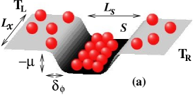
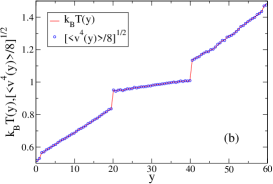
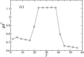
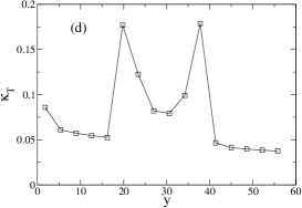
Figure 1: (Color online) (a) A schematic diagram of the system showing the liquid and solid regions produced by the external chemical potential of depth $-\mu$. The various dimensions mentioned in the text are also marked in the figure. (b) Plot of temperature profile $k_{B}T(y)$ and fourth moment of velocity $m\sqrt{\langle v^{4}(y)\rangle/8}$ at $\mu=13$. (c) The local density profile along $y$-direction at $\mu=13$. (d) The isothermal compressibility $\kappa_{T}$ as a function of $y$ at $\mu=13$. Compressibility shows strong peaks near the interfaces. Due to small size, interfacial enhancement of compressibility permeates right through the whole of solid region. In (c) and (d) lines are guides to eye.

3 Results

The system is first allowed to reach the steady state in a temperature gradient with the two walls at right and left being maintained at temperatures of $k_{B}T_{R}=1.5$ and $k_{B}T_{L}=0.5$ such that the current density integrated over the whole $x$-range is the same at all $y$. The local temperature can be defined as $k_{B}T(y)=\langle 1/2~{}mv^{2}(y)\rangle$, where the averaging is done locally over strips of width $d=1$ and length $L_{x}$. If local thermal equilibrium (LTE) is maintained we should have, $\langle v^{4}(y)\rangle=8(k_{B}T(y)/m)^{2}$. We find $k_{B}T(y)$ and $\langle v^{4}(y)\rangle$ as a function of distance $y$ from cold to hot reservoir (Fig. 1(b)). From Fig. 1(b) it is evident that the temperature profile is almost linear in the single phase regions, with sharp increase near the interfaces and LTE is approximately valid in all regions. With increased $\mu$, the temperature difference between the edges of the solid region decreases indicating an enhancement of heat conductance within the solid. The temparature jumps at the interfaces is a measure of the Kapitza or contact resistance ($R_{K}$)[12] defined as,

$$R_{K}=\frac{\Delta{T}}{j_{E}}$$ (2)

where $\Delta{T}$ is the difference in temperature across the interface. The Kapitza resistance increases with increasing trapping potential. It is evident that the interfaces are the regions of the highest resistance in the system. This large resitance can be traced back to large density mismatch at the contact of two phases. In Fig.1(c) we plot the local density profile $\rho(y)d^{2}$. The trapping region shows large density corresponding to the solid. Also the colder liquid near the reservoir on the left shows a larger density than the hotter liquid near the one on the right. In Fig.1(d) we plot the local compressibility $\kappa_{T}(y)$ defined via $\kappa_{T}=\rho^{-2}(\partial\rho/\partial\mu)_{T}$. Surprisingly, the compressibility of the interfaces is very large making the narrow solid region also unusually compressible pointing to the presence of large local number fluctuation.

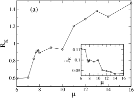
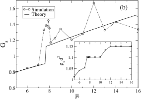
Figure 2: (left)(a)Plot of the Kapitza resistance, $R_{K}$, expressed in units of $\tau_{s}d$ as a function of the potential depth $\mu$, shows a jump at the layering transition. (right)(b) Plot of the thermal conductance of the solid region, $G_{s}$ [in units of $(\tau_{s}d)^{-1}$] as a function of $\mu$. The points denote simulation data and the solid line a free volume type calculation of heat conductance $[G_{s}]_{fv}$. The inset shows the corresponding change in solid density $\rho_{s}d^{2}$.

In Fig. 2(a) we have plotted the Kapitza resistance $R_{k}$ across the solid liquid interface, averaged over the two interfaces, as a function of the strength of the external potential $\mu$. The inset of Fig. 2(a) shows the heat flux through the system as a function of $\mu$. As $\mu$ increases, the atoms from the surrounding liquid get attracted into the potential well and the density of the liquid becomes lower. The density mismatch at the solid-liquid interface therefore increases progressively. This figure shows fairly sharp increase in $R_{k}$ as well as sharp decrease in current density $j_{E}$ near $\mu=8$ and $12$. As we will see later, these are the $\mu$ values at which the solid undergoes two types of layering transitions.

In Fig.2(b) we show the heat conductance in the solid region $G_{s}$ as a function of strength of the trapping potential $\mu$. The inset in Fig.2(b) shows the change in the averaged density of the solid region $\rho_{s}d^{2}$. The thick solid line in Fig.2(b) is an analytical estimate obtained from a free volume type calculation[17] to be discussed in the next section. The $\rho_{s}d^{2}-\mu$ plot shows clear staircase-like sharp increases near the same values of $\mu$ ($\approx$ 8 and 12) where sharp changes in thermal conductance occur. With increase in the strength of the trapping potential, we observe two modes of density enhancement: (A) A whole layer of particles enter to increase the number of lattice planes in $y$-direction. This happens, e.g., as $\mu$ is increased from $7$ to $8$. Thus in this mode the separation of lattice planes parallel to the liquid-solid interface decreases (see Fig.3(a)). (B) Each of the lattice planes parallel to the interface grow by an atom thereby decreasing the interatomic separation within each lattice plane. This happens, e.g., as one increases $\mu$ from $10$ to $12$ (see Fig.3(c)). These two modes of density fluctuations leave their signatures by enhancing the heat conductance $G_{s}$ - the effect of A being more pronounced than that of B.

With increase in $\mu$, these two modes alternate one after another, allowing the system to release extra stress developed due to particle inclusion in one direction in one cycle, by inclusion of particles in the perpendicular direction in the next cycle. Finally, at large enough $\mu$ the density of the solid region saturates ending the cycles. It is also interesting to observe, how the particles accomodate themselves going from Fig.3(a)-(d). We find strained triangular solids with $23\times 23$, $24\times 23$ and $24\times 24$ unit cells at $\mu=8,12$ and $24$ respectively (See Fig.3). In the intermediate configurations one observes metastable dislocation pairs (Fig3(d)) and peaks in the local particle density which corresponds to a few particles rapidly oscillating between two neighbouring positions (Fig3(b)) in order to maintain commensurability. Such rapid, localized, particle fluctuations may be observable in experiments.

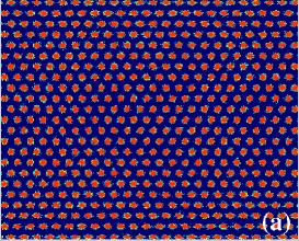
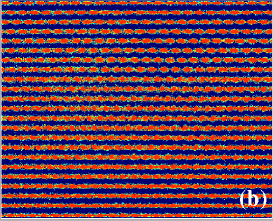
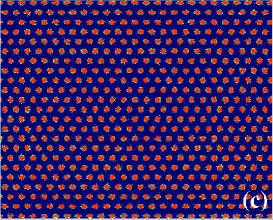
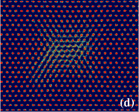
Figure 3: (Color online) Overlapped density plot of $500$ configurations in the region trapped by external potential $\mu$: (a) A $23\times 23$ triangular lattice solid formed from a $23\times 22$ triangular lattice as the potential is increased from $\mu=7$ to $\mu=8$. (b) Local density peaks hop in $x$-direction to incorporate $>23$ particles in lattice planes in response to increased potential $\mu=11$. (c) A $24\times 23$ triangular lattice solid at $\mu=12$. Notice the increase in particle numbers in the lattice planes. (d) Configuration obtained after $1.5\times 10^{4}\delta t$ as a $24\times 23$ steady state solid at $\mu=16$ is quenched to $\mu=24$. This shows a dislocation pair – a $23$-layered region trapped in between a $24$-layered solid. At steady state (after a time $10^{5}\delta t$) dislocations annihilate to produce a $24\times 24$ triangular lattice solid. Color code: blue (dark): low density and red (light): high density.

The layering transition in the solid by process (A) occurs via metastable dislocation formation and annihilation by incorporating particles from the liquid region. The kinematics of dislocation generation, transport and decay is controlled by diffusion which is a very slow process[7] in a solid compared to particle collision and kinetic energy transfer times. Thus it is possible for a system with metastable dislocation pairs to reach an effective thermal steady state. Fig.3.(d) shows overlapped configurations of the solid region containing a dislocation-antidislocation pair, as the system is quenched from $\mu=16$ to $\mu=24$. The overlapped configurations are separated by time $100\,\delta t$ and collected after a time of $1.5\times 10^{4}\,\delta t$ after the quench. At this stage the system is in a metastable state though, at the same time, maintaining LTE that we check by computing $\langle v^{4}(y)\rangle$ and $k_{B}T(y)$ locally. This gives a heat conductance $G_{s}=2.29\,(\tau_{s}d)^{-1}$. After a further wait for $10^{5}\,\delta t$ the dislocations get annihilated. At this stage the whole solid region is transformed into an equilibrium $24\times 24$-triangula lattice. On measuring the heat conductance now, we obtain $G_{s}=3.53\,(\tau_{s}d)^{-1}$. Thus with the annihilation of a single dislocation pair the conductance of the solid rises by about $54\%$! Metastable configurations with dislocation pairs, therefore, have strikingly different thermal properties in this small system. Note that in the present system, configurations containing dislocations are always metastable since dislocations are either annihilated or are lost at the interface[2].

4 Free volume heat conductance

Finally, we provide a brief sketch of an approximate theoretical approach for calculating heat conductance within the solid region. A detailed treatment of this approach is available in Ref.[17]. The continuity of the energy density can be utilized to obtain an exact expression for $\alpha$-th component of the heat flux density

$$j_{\alpha}({\bf r}) = j_{\alpha}^{K}({\bf r})+j_{\alpha}^{U}({\bf r})$$ (3)

$$= \sum_{i}\delta({\bf r}-{\bf r}_{i})h_{i}{\bf v}_{i}^{\alpha}+\frac{1}{2}\sum_{i,j\neq i}\theta(x_{i}^{\alpha}-x^{\alpha})\prod_{\nu\neq\alpha}\delta(x^{\nu}-x_{i}^{\nu})f_{ij}^{\beta}(v_{i}^{\beta}+v_{j}^{\beta}).$$

Here $\theta(x)$ is the Heaviside step function, $\delta(\dots)$ is a Dirac delta function, $h_{i}=m{\bf v}_{i}^{2}/2+\phi({\bf r}_{i})+\sum_{i>j}u(r_{ij})$, $\phi({\bf r}_{i})$ is an onsite potential and $u(r_{ij})$ is inter-particle interaction. The first term in Eq.3, $j_{\alpha}^{K}({\bf r})$, denotes the amount of energy carried by particle flux (convection) and $j_{\alpha}^{U}({\bf r})$ denotes the net rate at which work is done by particles on the left of $x^{\alpha}$ on the particles on the right (conduction). The $\alpha$-th component of the integrated heat current density over the solid region is,

$$\langle I_{\alpha}\rangle=\sum_{i}\langle~{}h_{i}v_{i}^{\alpha}\rangle-\frac{1}{4}\sum_{i,j\neq i}\left\langle~{}\frac{\partial u(r_{ij})}{\partial r_{ij}}\frac{x^{\alpha}_{ij}x^{\beta}_{ij}}{r_{ij}}(v_{i}^{\beta}+v_{j}^{\beta})~{}\right\rangle.$$ (4)

In this study we focus on the average heat current density along $y$-direction, $j_{E}=\langle I_{y}\rangle/L_{x}L_{s}$. We assume LTE and ignore conductance inside solid [17]. Then assuming the conductance of our present system to be simply proportional to that of a hard disk system with an effective diameter $\sigma$, the heat conductance in units of $(\tau_{s}d)^{-1}$ can be expressed as,

$$G_{s}=\frac{j_{E}}{\Delta T}=\left[3\frac{\rho_{s}}{L_{s}}\frac{y_{c}^{2}}{\tau_{c}}\right]\left(\frac{d}{\sigma}\right)^{2}$$ (5)

where $\rho_{s}$ is the average density of the solid, $y_{c}$ is the average separation between the colliding particles in $y$-direction and $\tau_{c}$ is the mean collision time. The extra factor of $(d/\sigma)^{2}$ is due to the mapping of the soft disks of diameter $d$ to effective hard disks of diameter $\sigma$.

We estimate $y_{c}^{2}$ and $\tau_{c}$ from the fixed neighbor free volume theory as in Ref.[17]. Briefly, we assume that a (hard) test particle moves in the fixed cage formed by the average positions of its neighbors and obtain the average values $[y_{c}^{2}]_{fv}$ from geometry and the timescale $[\tau_{c}]_{fv}=c\sqrt{V_{fv}/k_{B}T}$ where $V_{fv}$ is the available free volume of the test particle moving with a velocity derived from the temperature $k_{B}T$. The effective hard disk diameter $\sigma$ and the constant $c$ of ${\cal O}(1)$ are both treated as fitting parameters. Using $k_{B}T=1$, $d/\sigma=1.13$ and $c=0.4$ we obtain a fit to the $G_{s}-\mu$ curve with a layering transition from $22$ to $23$ layers near $\mu=8$. The fitted result, depicted as the solid line in Fig2(b), is seen to reproduce most of the qualitative features of the simulation results, especially the jump in conductance due to the layering transition.

5 Conclusion

We have shown that details of the structure have a measurable effect on the thermal properties of the trapped solid lying in contact with its liquid. In this study, we were particularly interested in exploring the impact of structural changes, viz. the layering transitions, on heat transport. One must, however, remember that, the layering transition is a finite size effect[2] and gets progressively less sharp as one goes to very large channel widths. An important consequence of this study is the possibility that the thermal resistance of interfaces may be altered using external potential which cause layering transitions in a trapped nano solid. We have shown that metastable dislocations drastically reduce the conductance of an otherwise defect free nano sized solid. Recently, electrical [18] and thermal [17] transport studies on confined solid strips have also revealed strong signatures of such structural transitions due to imposed external strain. We believe that these phenomena have the potential for useful applications e.g. as tunable thermal switches or in other nano engineered devices.

References

- [1] D. G. Cahill et al., J. Appl. Phys. 93, 793 (2003).
- [2] A. Chaudhuri, S. Sengupta, and M. Rao, Phys. Rev. Lett. 95, 266103 (2005).
- [3] H. J. Metcalf and P. van der Straten, Laser Cooling and Trapping (Springer, Heidelberg, 1999).
- [4] W. D. Phillips, Rev. Mod. Phys. 70, 721 (1998).
- [5] D. G. Grier, Nature 424, 810 (2003).
- [6] R. Haghgooie and P. S. Doyle, Phys. Rev. B 70, 061408 (2004).
- [7] D. Chaudhuri and S. Sengupta, Phys. Rev. Lett. 93, 115702 (2004).
- [8] A. Ricci, P. Nielaba, S. Sengupta, and K. Binder, Phys. Rev. E 74, 010404 (2006).
- [9] P. G. de Gennes, Langmuir 6, 1448 (1990).
- [10] J.-L. Barrat and F. Chiaruttini, Molecular Physics 101, 1605 (2003).
- [11] P. L. Kapitza, J. Phys. U.S.S.R. 4, 181 (1941).
- [12] G. L. Pollack, Rev. Mod. Phys. 41, 48 (1969).
- [13] A. Lippi and R. Livi, J. Stat Phys. 100, 1147 (2000).
- [14] F. Bonetto, J. Lebowitz, and L. Rey-Bellet, in Mathematical Physics 2000, edited by A. Fokas et al. (Imperial College Pres, London, 2000), p. 128.
- [15] P. Grassberger and L. Yang, (2002), arXiv:cond-mat/0204247.
- [16] D. Frenkel and B. Smit, Understanding Molecular Simulation, 2nd ed. (Academic Press, New York, 2002).
- [17] D. Chaudhuri and A. Dhar, Phys. Rev. E 74, 016114 (2006).
- [18] S. Datta, D. Chaudhuri, T. Saha-Dasgupta, and S. Sengupta, Europhys. Lett. 73, 765 (2006).