Numerical analysis of the quantum dots on off-normal incidence ion sputtered surfaces

Abstract

We implement substrate rotation in a 2+1 dimensional solid-on-solid model of ion beam sputtering of solid surfaces. With this extension of the model, we study the effect of concurrent rotation, as the surface is sputtered, on possible topographic regions of surface patterns. In particular we perform a detailed numerical analysis of the time evolution of dots obtained from our Monte Carlo simulations at off-normal-incidence sputter erosion. We found the same power-law scaling exponents of the dot characteristics for two different sets of ion-material combinations, without and with substrate rotation.

I INTRODUCTION

The size-tunable atomic-like properties of (e.g. II-VI and III-V) semiconductor nanocrystals have diverse applications. These properties arise from the quantum confinement of electrons or holes in the quantum dots (QDs) to a region on the order of the electrons’ de Broglie wavelength. Examples of the applications can be found in solid-state quantum computation Gershenfeld and Chuang (1998) and in electronic and opto-electronic devices like diode lasers, amplifiers, biological sensors, electrolumniscent displays, and photovoltaic cells. Colvin et al. (1994); O’Regan and Grätzel (1991)

A more recent method of fabrication is the sputtering of semiconductor surfaces with a beam of energetic ions impinging at an angle $\theta$ with respect to the direction perpendicular to the surface. Facsko et al. (1999) This has been shown to be a cost-effective and more efficient means of producing uniform high-density semiconductor nanocrystals, Facsko et al. (1999); Frost et al. (2000); Facsko et al. (2001); Gago et al. (2001) in contrast to previous methods such as epitaxy, lithographic techniques, colloidal synthesis, electrochemical techniques, and pyrolytic synthesis.

Using the continuum theory, it was shown that QD formation by $\theta=$ 0 sputtering is restricted to a very narrow region of the parameter space. Kahng et al. (2001); Frost (2002) It has also been shown that dot formation is possible for $\theta>$ 0, within a broader region, under concurrent sputtering and sample rotation.Frost (2002) Using a simple discrete solid-on-solid model, which includes the competing processes of surface roughening via sputtering and surface relaxation via thermal diffusion, we recently found that for $\theta>$ 0, without sample rotation, a dot topography is only one among other possible topographies which may arise. The type of the emerging topography depends on the longitudinal and lateral straggle of the impinging ion as it dissipates its kinetic energy via collision cascades with atoms within the material. Yewande et al. (2006)

In this study, we implement sample rotation in the simulation model along the lines of Refs. Bradley and Cirlin, 1996 and Bradley, 1996. For varying values of the ion parameters we find different kinds of surface patters, including dots. The dots are similar to those obtained without sample rotation, but the underlying oriented ripple structures are lacking. We study the time evolution of dots emerging from oblique ion incidence in more detail, performing simulations for two different sets of parameters, corresponding to two different materials (GaAs sputtered with Ar and Si sputtered with Ne) with and without rotation. We found that without rotation the average number of dots decreases with increasing fluence, but stays approximately constant for a rotated sample. Furthermore the uniformity of dots is greatly enhanced by sample rotation. Remarkably, both materials exhibit the same scaling of the dot characteristics with sputter time.

The rest of the paper is organized as follows: In section II we shall briefly review the continuum theory of sputtered amorphous surfaces. In section III we shall give a brief description of the discrete simulation models applied in this work. In section IV we study the effect of rotation on the possible topographies reported in Ref. Yewande et al., 2006; expecially off-normal incidence dot formation. Finally, in section V, we shall present and discuss our results of the analysis of dot topographies.

II CONTINUUM THEORY

In the seminal theory of P. Sigmund on ion-beam sputtering of amorphous and poly-crystalline targets, it was shown that the spatial energy distribution $E({\bf r})$ of an impinging ion may be approximated by a two-dimensional Gaussian of widths $\sigma$ and $\mu$, parallel ($z^{\prime}$-axis) and perpendicular ($x^{\prime},y^{\prime}$-axes) to the ion beam direction, respectively Sigmund (1969); Bradley and Harper (1988),

$$E({\bf r}^{\prime})=\frac{\epsilon}{(2\pi)^{3/2}\sigma\mu^{2}}\exp\biggl{(}-\frac{[z^{\prime}+a]^{2}}{2\sigma^{2}}-\frac{x^{\prime 2}+y^{\prime 2}}{2\mu^{2}}\biggr{)}\,,$$ (1)

where $\epsilon$ is the total energy of an impinging ion and $a$ the average penetration depth.

When describing the surface by a two-dimensional height field $h({\bf r},t)$ (solid-on-solid description), the normal erosion velocity $v=-[1+(\nabla h)^{2}]^{-1/2}\partial_{t}h$ at the point ${\bf r}=(0,0,0)$ is proportional to the total power transported to this point by the ions of the impinging ion beam. It may be expressed as Cuerno and Barabási (1995); Makeev and Cuerno (2002)

$$v=p_{c}\int_{R}d{\bf r}\Phi({\bf r})E({\bf r}).$$ (2)

The integral is taken over the region $R$ containing all the points at which the deposited energy contributes to the total power at ${\bf r}=0$ and $p_{c}$ is a proportionality constant.Makeev and Cuerno (2002) $\Phi({\bf r})$ is a local correction to the uniform flux $J_{f}$. Note that shadowing effects among neighboring points and redeposition of eroded material are ignored.

By standard arguments, an equation for the evolution of the surface height field $h(x,y,t)$ due to sputtering can be derived from Eq. (2), which takes on the form Bradley and Harper (1988); Cuerno and Barabási (1995)

$$(\partial_{t}h)_{S}\approx-v_{f}+v_{f}^{\prime}\partial_{x}h+\nu_{x}\partial^{2}_{x}h+\nu_{y}\partial^{2}_{y}h$$

$$+\frac{\chi_{x}}{2}(\partial_{x}h)^{2}+\frac{\chi_{y}}{2}(\partial_{y}h)^{2}+\eta_{S}({\bf r},t),$$ (3)

where the $x$-axis is parallel to the ion beam direction, $v_{f}$ is the erosion velocity of a flat surface and $\nu_{x}(\theta,\sigma,\mu)$ [$\nu_{y}(\theta,\sigma,\mu)$] is the surface-tension coefficient along [perpendicular to] the ion beam direction. Depending on the parameters $\theta,\sigma,\mu$, the quantity $\nu_{x}$ can exhibit positive as well as negative values, whereas $\nu_{y}$ is always negative. $\chi_{x}$ and $\chi_{y}$ are the coupling constants of the dominant non-linearities along the respective directions. $\eta_{S}$ is an uncorrelated noise term, with zero mean. This term represents the random arrival of the ions onto the surface.

The surface height also evolves due to surface particles hopping from one point to the other. On a coarse-grained level this can be described by the continuity equation for the conserved particle current

$$(\partial_{t}h)_{D}=-\nabla\cdot{\bf j}+\eta_{D}({\bf r},t),$$ (4)

where the local current density ${\bf j}$ is a function of the derivatives of $h$; i.e, ${\bf j}$ = ${\bf j}[\nabla^{m}h,(\nabla h)^{n}]$ ($m$ and $n$ are integers), and the acceptable functional form is subject to symmetry constraints. $\eta_{D}$ reflects the randomness inherent in the surface-diffusion process. A commonly studied example of a surface migration model is the Mullins-Herring model, which leads to the particularly simple form $\nabla\cdot{\bf j}=D\nabla^{4}h$ for the current density.Kim and Sarma (1994)

Thus, considering Eqs. (II) and (4), the time evolution of a sputtered surface is governed by a Kuramoto-Sivashinsky type equation

$$\partial_{t}h=-v_{f}+v_{f}^{\prime}\partial_{x}h+\nu_{x}\partial^{2}_{x}h+\nu_{y}\partial^{2}_{y}h+\frac{\chi_{x}}{2}(\partial_{x}h)^{2}$$

$$+\frac{\chi_{y}}{2}(\partial_{y}h)^{2}-D\nabla^{4}h+\eta({\bf r},t).$$ (5)

The exact form of each coefficient of Eq. II is given in Ref. Makeev and Cuerno, 2002 and will be used later in the analysis of our results (see Fig. (5) in section (III)).

The anisotropy ($\nu_{x}\neq\nu_{y}$, $\chi_{x}\neq\chi_{y}$) arises from the oblique incidence which leads to different erosion rates (or different rates of maximizing the exposed area) along parallel and perpendicular directions relative to the ion beam direction. From the linearized Eq. (II) it is easy to see that periodic ripples are growing with wavevector ${\bf k}=\sqrt{\max(|\nu_{x/y})|/2D}$ driven by the dominant negative surface tension. These ripples are stabilized by the surface diffusion term. With prolonged sputtering surface slopes become too big to neglect the nonlinear terms and the ripples are destroyed, after which a new rotated ripple structure may emerge. Park et al. (1999)

If the sputtered substrate is rotated with sufficiently large angular velocity, Yewande or if $\theta=$ 0, no externally induced relevant anisotropy is present. In this case ripples do not develop for the class of materials we study here and the relevant evolution equation is the isotropic version of Eq. (II), which predicts cellular structures of mean width $\sim(D/|\nu|)^{1/2}$ and mean height $\sim|\nu|/|\chi|$.Bradley (1996) According to Ref. Kahng et al., 2001, these cellular structures eventually evolve to either a dot topography ($\chi>$0) or a hole topography ($\chi<$0); which explains the normal incidence dotFacsko et al. (1999); Gago et al. (2001); Facsko et al. (2001) and holeRusponi et al. (1998, 1999) topographies found in previous experiments.

Thus, one would expect oblique incidence dot formation to result from isotropic sputtering induced by substrate rotation. However, in our recent simulations Yewande et al. (2006) we found dot topographies without sample rotation, though with some underlying (anisotropic) ripples oriented parallel to the ion beam direction. We found that the oblique incidence dots arise from a dominance of the ripples oriented parallel to the ion beam direction, over those with a perpendicular orientation; the dots being the remains of such perpendicular ripples (see Fig. 2 below) after long times.

In the next chapter we will outline the simulation method we have used in Ref. Yewande et al., 2006 and which we have extended to the case with rotation as presented in this work.

III MONTE CARLO SIMULATION

To simulate the competing processes discussed in section II on a discrete system, we use the Monte Carlo model of sputter erosion introduced in Ref. Hartmann et al., 2002 (HKGK model). To make the paper self-contained, we provide some details here. We simulate the sputtering process on an initially flat surface of size $L^{2}$ with periodic boundary conditions, by starting an ion at a random position in a plane parallel to the initial surface, and projecting it along a straight trajectory inclined at angle $\theta$ to the direction perpendicular to the averaged surface configuration and at an azimuthal angle $\phi$. An ion penetrates the solid through a depth $a$ and releases its energy according to Eq. (1). An atom at a position $(x,y,h)$ is eroded (see Fig. 1) with probability proportional to $E({\bf r^{\prime}})$ given in Eq. (1). It should be noted that, in accordance with the assumptions of the theoretical models Makeev and Cuerno (2002); Bradley and Harper (1988); Cuerno and Barabási (1995), this sputtering model neglects evaporation, redeposition of eroded material and preferential sputtering of surface material at the point of penetration. The surface is defined by a single valued, discrete time dependent SOS height function $h({\bf r},t)=h(x,y,t)$. The time t is measured in terms of the ion fluence; i.e, the number of incident ions per two-dimensional lattice site $(x,y)$. The choice of the parameters $\sigma,\mu$ and $\theta$ is discussed below. Substrate rotation, at constant angular velocity $\omega\geq\nu^{2}/D$, is implemented by keeping the substrate static and then rotating the ion beam instead, which is equivalent to keeping the ion beam direction fixed and rotating the substrate Bradley and Cirlin (1996). In our simulations we choose $\phi$ randomly from the interval $0\leq\phi<2\pi$, since, in the large $\omega$ limit the solid appears to be sputtered from all angles $\phi$.Bradley (1996)

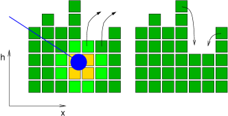
Figure 1: The model consists of a square field of discrete height variables $h(x,y)$, corresponding to piles of $h(x,y)$ particles at position $(x,y)$. Here a projection to the $h-x$ is shown. Left: Each ion impact is modeled by an distribution describing the energy deposited by the ion. Atoms on the surface are removed with a probability proportional to the energy. Right: Surface diffusion; by decreasing height differences the energy is decreased.

Our model of the sputtering mechanism sets the time scale of the simulation in a way, which allows direct comparison with experiments. Any relevant surface diffusion mechanism may be combined with this sputtering model. Yewande Here, we use a realistic solid-on-solid model of thermally activated surface diffusion Smilauer et al. (1993). Surface diffusion is simulated as a nearest neighbor hopping process with an Arrhenius hopping rate

$$R(E,T)=R_{0}\exp(-E/k_{B}T),$$ (6)

where $R_{0}=k_{B}T/\hbar$, and $T$ is the effective substrate temperature (see below). The energy barrier $E=E_{vn}+n_{n}E_{ln}+E_{se}$ consists of a substrate term ($E_{vn}=$0.75 eV), a nearest neighbor term ($E_{ln}=$0.18 eV), and a step barrier term ($E_{se}=$0.15 eV), which only contributes in the vicinity of a step edge, and is zero otherwise. In each diffusion sweep all surface particles are considered, and those that are not fully coordinated may hop to a neighboring site. Note that we have to use a higher effective temperature Yewande et al. (2005) in our simulation in order to account for the greatly enhanced surface diffusion due to thermal spikes. A thermal spike is a series of sharp peaks and minima in the spatio-temporal distribution of the surface temperature, arising from the occurence of local heating of the surface right after every ion impact, followed by rapid cooling. Hence, we have used a higher effective temperature $k_{B}T=$0.1 eV, which was estimated in our previous work and which roughly corresponds to experimental sputtering at room temperature.

The model captures the essential features of sputtered surfaces at nanometer lengthscales; especially nonlinear effects Hartmann et al. (2002); Yewande et al. (2005). Although a direct mapping of this model to the continuum equations is unavailable, the model is expected to be consistent with variants of the KS equation. Yewande et al. (2006); Lauritsen et al. (1996)

IV EFFECT OF ROTATION ON THE TOPOGRAPHIES

In this study, a lattice of linear size $L$ = 128 is used with a lattice spacing corresponding roughly to a distance of 0.5 nm. The simulated time is set such that 1 ion/atom corresponds to an ion fluence of 3$\times$10¹⁴ ions/cm². We use a sputter yield of about 7 surface atoms/ion, as compared to 5 SiO₂ molecules/ion (reduced to 0.1 SiO₂ molecules/ion with H ion) and 0.3-0.5 molecules/ion in the experiments of Refs. Mayer et al., 1994 and Habenicht et al., 1999 respectively; this may result in lengthscales differing from those of the cited experiments, but we found in our previous studies Hartmann et al. (2002); Yewande et al. (2005, 2006) that predicted universal features exist, which are directly comparable to experimental results. We will subsequently discuss such features for rotated samples.

In Ref. Yewande et al., 2006 six regions with different topographies (including e.g, smooth, hole, and dot regions) were shown to emerge for ion collisional parameters $a$ = 6, 0 $\leq\sigma\leq$ 5, 0 $\leq\mu\leq$ 5 (all measured in units of lattice spacings), at time $t$ = 3 ions/atom. In this section we study the effects of sample rotation on these topographies, in particular effects on the region with dot topography. The differences in topographies between rotated and unrotated samples are visualized in Fig. 2 and Fig. 3, for $a$ = 6, $t$ = 3, and $\theta$ = 50^∘.

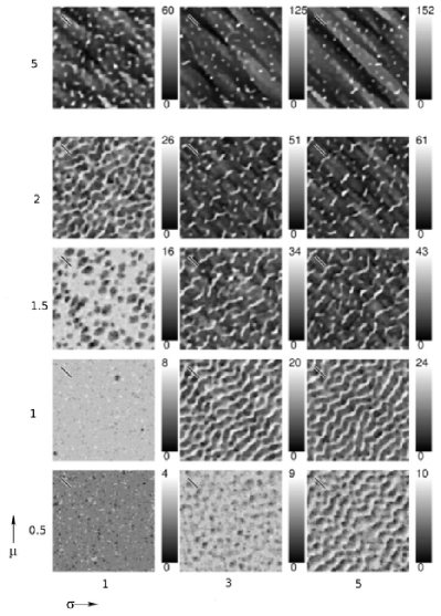
Figure 2: Possible topographies of the model, within the experimental constraints considered in Ref. Yewande et al., 2006. $t=$ 3, $a=$ 6, $\theta=$ 50^∘. Left - right columns: $\sigma$ = 1, 3, and 5, respectively. Bottom row - top row: $\mu$ = 0.5, 1, 1.5, 2, and 5, respectively. The last two profiles of the top row belong to the dot region (region V) of Ref. Yewande et al., 2006.

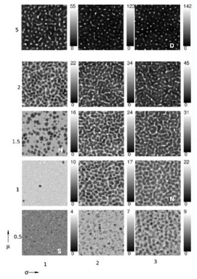
Figure 3: Profiles obtained from simultaneous sputtering and rotation, using the same parameters as in Fig. 2. $t=$ 3, $a=$ 6, $\theta=$ 50^∘. Left - right columns: $\sigma$ = 1, 3, and 5, respectively. Bottom row - top row: $\mu$ = 0.5, 1, 1.5, 2, and 5, respectively. The last two profiles of the top row belong to the dot region (region V) of Ref. Yewande et al., 2006. Structure factors of the lettered profiles are provided in Fig. 4 [S - (relatively) smooth; H - hole; N - non-oriented structures; D - dot].

As seen from Fig. 3 (and Fig. 4, see below), no anisotropy can be found with substrate rotation, as expected from the continuum theory. The ripple structures obtained for $\mu\leq$ 2 (Fig. 2) do not appear for rotated substrates. The underlying parallel ripples of the dot region (topmost row of Fig. 2) are also absent for rotated substrates. However, hole formation is not suppressed, we get holes with as without rotation as is visible in Fig. 2. This fact can be understood from the continuum theory, which predicts roughly equal erosion rates along both directions for parameters in the hole region,Yewande et al. (2006) hence there is no anisotropy to be destroyed. Furthermore, ripple patterns perpendicular with resepct to the ion beam direction are replaced by non-oriented structures, and the ordered parallel ripples are no longer present if the substrate is rotated. (see Fig. 3),

For a closer inspection, we calculate the structure factors, $S({\bf k},t)=|h({\bf k},t)|^{2}$ from the Fourier transform $h({\bf k},t)$ of the height field $h({\bf r},t)$. In particular we consider four prototypical topographies marked by letters S, H, N, D in Fig. 3. S stands for “relatively smooth”, H for “hole”, N for “non-oriented structures”, and D for “dots”. The results are shown in Fig. 4. As can be seen from this figure, and as expected, there is no anisotropy visible in all cases. In the case of the relatively smooth surface S, there is also no characteristic lengthscale. For the hole topography, H, there is still no specific lengthscale but there now exists an upper bound $k_{ub}$ on $|{\bf k}|$ due to the presence of the holes. On the surface with non-oriented structures (N) a well defined lengthscale with $k_{ub}$ as well as a lower bound $k_{lb}$ can be found. And finally, in the case of the dot topography (D), we also have a characteristic lengthscale, but $k_{lb}$ is shorter here than for the N topography, which implies that the average separation of the dots is larger than that of the non-oriented structures, as expected from Fig. 3.

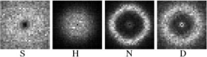
Figure 4: Structure factor of the lettered surface profiles in Fig. 3. S $\Rightarrow$ (relatively) smooth; H $\Rightarrow$ hole; N $\Rightarrow$ non-oriented structures; D $\Rightarrow$ dot. ${\bf k}={\bf 0}$ at the centre; and ${\bf k}=\frac{2\pi}{8}(\pm 1,\pm 1)$ at the corners.

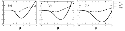
Figure 5: The coefficients, $\nu_{av}$ and $\chi_{av}$, of the isotropic version of Eq. II, Bradley (1996) for the rotated case, as functions of $\mu$. (a) $\sigma=$ 1.0, (b) $\sigma=$ 3.0, and (c) $\sigma=$ 5.0.

According to the continuum theory, there exists a single effective surface tension coefficient $\nu_{av}$ = $\nu_{x}$ + $\nu_{y}$ and a single nonlinear couplingBradley (1996) $\chi_{av}$ for all directions in rotated samples, since there is no anisotropy left in the system. Fig. 5 shows a plot of these coefficients based upon the explicit expressions in Ref. Makeev and Cuerno, 2002. As can be seen from Fig. 5 and Eq. (II) the surface roughens with time, with smaller $\nu_{av}$ ($\nu_{av}<$0) corresponding to higher roughness. Surfaces in the parameter range for which 0$>\nu_{av}\gg$ -1, are relatively smooth (S) topographies.

Figure 6: Surface roughness, $W$, with dots excluded. Main plot: $W$ as a function of $\mu$ for $\sigma=$ 5. Inset: $W$ as a function of $\sigma$ for $\mu=$ 5. $t=$ 3 ions/atom.

Considering Fig. 5, one sees that $|\nu_{av}|$ first increases, in accordance with the increasing height difference on the greyscale charts on the profiles of Fig. 3 and then it decreases as we tend towards the dot region. These changes in the roughness are not visible on the greyscale charts due to the appearance of the dots, which are considerably higher than an average surface protrusion in the dot-free profiles. Therefore we have also studied the surface roughness, with the dots excluded, as shown in Fig. 6 (Details of our dot-isolation method are discussed in the next section). In this figure, the roughness $W$ as a function of $\mu$ ($\sigma=$ 5) is shown in the main plot, where the roughness first increases and than decreases again, in accordance with the continuum theory. The inset shows a plot of $W$ versus $\sigma$, for $\mu=$ 5.

Figure 7: Time evolution of the relatively smooth topography of Fig. 2 with rotation. $\sigma=$ 3, $\mu=$ 0.5. (a)-(d): $t=$ 3, 40, 90, and 150, respectively.

When the local surface slopes become significant (with prolonged sputtering), nonlinearities become relevant. It has been shown that for $\theta=$ 0 crossover to the nonlinear regime either gives rise to dot formation (if $\chi_{av}>$ 0) or hole formation (in case $\chi_{av}<$ 0) if ion-induced effective surface diffusion is the dominant relaxation mechanism Kahng et al. (2001). This is consistent with our results for parameters at which $\chi_{av}>$ 0 in Fig. 5 (i.e, for $\mu\gtrsim$ 3). We also found holes for $\chi_{av}<$ 0 (“H” region), but hole formation for long times is not as widespread as Fig. 5 seems to indicate. In particular, the hole topography eventually evolves into cellular structures similar to those shown in Fig. 7 at long times. Since $\nu_{av}\neq$ 0, the surface roughening is not wavelength independent, which explains the presence of the non-oriented protrusions.

For very small longitudinal and lateral straggle, $\sigma\leq$ 1, $\mu\leq$ 0.5, i.e. in the “S” region, we did not find any structure up to the longest simulation times. Note that with increasing $\sigma$, the $|\nu_{av}|\approx$ 0 interval is reduced.

For non-oriented structures “N”, simulations at longer times reveal only slight changes in the structures; no dot formation (see Fig. 8) appears. Hence, we have only observed dots with rotation wherever they can be found without rotation.

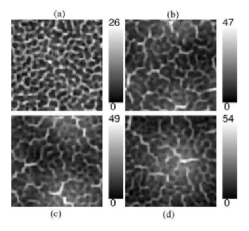
Figure 8: Time evolution of the non-oriented structures arising from rotation of rippled region of Fig. 2. $\sigma$ = 3, $\mu$ = 1.5. (a) - (d): $t$ = 3, 40, 90, and 150, respectively.

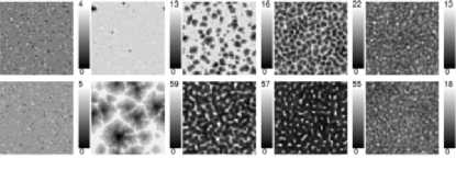
Figure 9: Topography changes as a result of changing the angle of incidence $\theta$, for $\sigma=$ 1; $\mu=$ 2 (top row), and 5 (bottom row). Top row, L-R: $\theta=$ 10, 30, 40, 50, 80. Bottom row, L-R: $\theta=$ 5, 10, 30, 50, 80.

When considering the emerging topographies of Fig. 3 at other angles of incidence, we found notable changes with $\theta$, as illustrated in Fig. 9 for $\sigma=$ 1, $\mu=$ 2 and $\sigma=1$, $\mu=5$). That is, changes from smooth $\to$ hole $\to$ non-oriented structure, and back to smooth (no structure) topographies appear. These changes imply that the roughness initially increases and then starts to decrease with increasing $\theta$ as shown in Fig. 10. In this figure $\sigma$ = 1 and data for $\mu$ = 2 and $\mu=5$ are represented by (black) circle and (red) square symbols, respectively. The behavior of the roughness with varying $\theta$ shown in Fig. 10 is in agreement with the experiments reported for Ar-ion sputtered rotating InP surfaces in Ref. Frost et al., 2000. But note that the roughness data reported in this experiment Frost et al. (2000) were obtained for an exposure time of 1200 secs., i.e.  in the steady state regime. To use such steady state values in Fig. 10 would require simulation times beyond our computational time constraints.

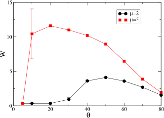
Figure 10: (Color online) Surface roughness $W$ as a function of $\theta$ for profiles shown in Fig. 9. Data for $\mu$ = 2 and 5 are represented by circle and square symbols, respectively. In both cases $\sigma$ = 1, $t$ = 3 ions/atom. Error bars are included, but they are much smaller than symbol size except at $\theta=10^{\circ}$ ($\mu=5$). For this case for about half of the runs the structure had already evolved to a non-oriented structure pattern with a considerable roughness, while the other half exhibited still a rather smooth surface. Hence, there seems to be a sharp transition in time from smooth to rough, where the transition time of finite samples fluctuates strongly.

V NUMERICAL ANALYSIS OF THE DOTS

Table 1: SRIM results for materials bombarded with noble gas ions.

Ion	Material	E/keV	$a$	$\sigma$	$\mu$
Ar	GaAs	1.6	6	5	3.8
Ar	Ge	1.6	6	5	3.8
Ne	Si	0.65	6	4.4	3.2

Focussing on topographic region “D” where dots have been found also without rotation, we obtained the experimental parameters corresponding to this region from SRIM simulations J.F. Ziegler and Littmark (1985) as shown in Table 1. We have performed two sets of simulations using the SRIM results: (i) 1.6 keV Ar ion sputtering of GaAs surfaces; where $a$ = 6, $\sigma$ = 5, $\mu$ = 3.8. (ii) 650 eV Ne ion sputtering of Silicon surfaces; where $a$ = 6, $\sigma$ = 4.4, $\mu$ = 3.2. In both cases we have used an ion beam inclination of $\theta=$50^∘ to the vertical.

In order to study the time evolution of dot characteristics (e.g. dot density, area, and height), we have used a similar clustering approach as in Ref. Yewande et al., 2005. A dot is defined as a cluster of points of local height maxima. This is done in two steps

• For any given time $t$ (we do not mention the time-dependence explicitly here) we consider the set of points

  $$M\equiv\{(x,y)|x,y\in(1,\cdots,L);h(x,y)\geq h_{c}\},$$ (7)

  where $L$ is the linear size of the system, $h_{c}$ is a cutoff height which the surface height at a point must equal/exceed for the point to be counted as (or part of) a dot. Yewande et al. (2005) We define $h_{c}$ to be a function of the average surface protrusion, which has the form: $h_{c}=h_{min}+p(\langle h\rangle-h_{min})$. Where $h_{min}$ is the lowest surface height, $\langle h\rangle$ is the average surface height, and $p$ is a fixed percentage.

• We call two points in $M$ neighbors if their distance is smaller than a given threshold $d_{c}$, we use $d_{c}=1$ here. Then, two points are called connected, if there exists a path from the first point to the other point such that all consecutive points along the path are neighbors. Now, each dot $D$ is a subset of $M$ (non-overlapping with any other dot) of maximum size such that all points in $D$ are mutually connected. Hence, dots are the transitive closures of the neighbor relation on $M$.

We start our simulations with a dot configuration obtained from a topography at $t=$ 3 ions/atom and we choose a value $p=p_{o}$ that yields the highest number of sampled dots $N_{o}$ (see Table 2). The initial clusters are shown in Fig. 11 for simulation of Ar-ion sputtering of GaAs without substrate rotation and with substrate rotation, respectively. The dot cross-section $A(D)$ is defined $A(D)=|D|$; i.e the cardinality of $D$. The average height $h_{d}$ of a single dot $D$ is defined as $h_{d}(D)=\frac{1}{|D|}\sum_{(x,y)\in D}h_{x,y}$. Note that, in order to exclude non-dot surface protrusions (see top row of Fig. 12) from our analysis, we have included an upper boundary of 50 cluster points (i.e $A(D)\leq$ 50) to our definition. In our analysis we only consider dots defined by these clusters. The results reported here are obtained from an average of 100 independent runs.

Table 2: Optimal parameters used to determine the cutoff height $h_{c}$

Simulation	$p_{o}$ (%)	$N_{o}$	State
Ar+ on GaAs	50	69	unrotated
Ar+ on GaAs	10	149	rotated
Ne+ on Si	60	76	unrotated
Ne+ on Si	20	139	rotated

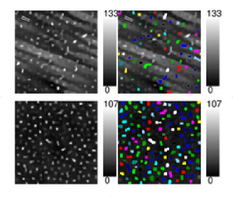
Figure 11: (Color online) Sample surface profiles for the unrotated case (top), and the rotated case (bottom) at t = 3 ions/atom. In the figures on the right the clusters formed from the corresponding profile on the left (as defined in the text) are printed on top of the profile. The scales indicate the surface height measured from the lowest height.

In Fig. 12, we show sample surface profiles without rotation (top row), and with rotation (bottom row), for simulation of 1.6 keV Ar-ion sputtering of GaAs. As can be seen from the top row of this figure, the ripples (with parallel orientation to ion beam direction) that coexist with the dots become more ordered with time, whereas the dots decrease in number with time; more analysis of these dots is provided below. On the other hand (bottom row of Fig. 12), these ripples do not exist when the substrate is subjected to concurrent rotation, and the density of the dots is more uniform.

In Fig. 13, we present results of the average number of sampled dots N_c, and the average dot height H${}_{c}=\overline{h_{d}}$, where the average is taken over all dots and all independent runs. The results of the average area of cross-section of the dots is presented in Fig. 14. In Figs. 13 and 14, open and closed circle symbols represent data obtained from Ar-GaAs with and without rotation respectively; while open and closed triangle symbols represent data obtained from Ne-Si with and without rotation respectively. The main result is that we found power law scaling of the dot characteristics with time; with or without rotation. In addition, we found the same scaling behavior for the two sets of simulation performed; i.e, 1.6 keV Ar ion sputtering of GaAs (Ar-GaAs), and 650 eV Ne ion sputtering of Si (Ne-Si).

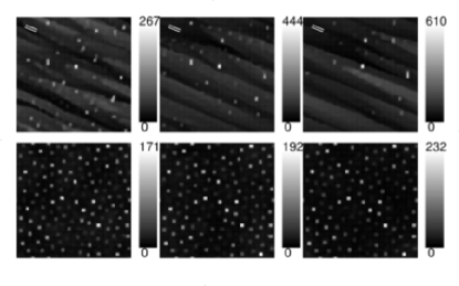
Figure 12: Surface profiles for the non-rotated (top row) and the rotated (bottom row) case. L - R, t = 10, 20, and 30 ions/atom respectively. The bar indicates the ion beam direction, and the scales indicate the surface height measured from the lowest height.

To be more specific, as can be seen from Fig. 13 (a), the average number of sampled dots decreases with time as N${}_{c}\sim t^{-\psi}$ for non-rotated samples, where $\psi=$ 0.583$\pm$0.007, while it stays approximately constant for rotated samples ($\psi\approx 0$). This indicates that the number of dots becomes insignificant without substrate rotation, so that one should use rotation if dot creation is the main purpose of the sputtering. Note that this result is already visible in Fig. 12 in qualitative form.

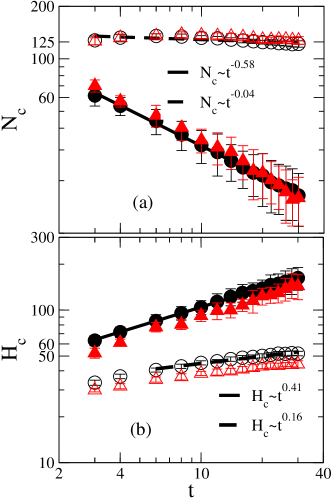
Figure 13: (Color online) Time evolution of (a) the average number N_c, and, (b) the average height H_c (both in lattice units), of the sampled dots with time (in ions/atom). Symbols: open and closed circle (triangle) symbols denote data obtained with and without substrate rotation respectively, for Ar-GaAs (Ne-Si).

On the other hand, as shown in Fig. 13 (b), the average height H_c increases with time as H${}_{c}\sim t^{\varrho}$, the increase is more rapid for the unrotated case ($\varrho=$0.409$\pm$0.004) than for the rotated case ($\varrho=$0.159$\pm$0.007). As expected, the dot height is lower with sample rotation due to the enhanced smoothening effect of the rotation. Bradley and Cirlin (1996); Bradley (1996) This smoothening also explains the higher initial number of dots for the rotated case [Fig. 13 (a)]: The dots that are not “visible” in the unrotated case, since they do not surmount the ripples, become “visible” in the rotated case since the rotation prevents ripple formation.

The mean cross sectional area A_c finally becomes almost time independent for both cases. However, as shown in Fig. 14 , an initial power law scaling A${}_{c}\sim t^{-\varsigma}$ occurs, which is more significant for the rotated case (where $\varsigma$ = 0.113$\pm$0.006) than for the unrotated case (where $\varsigma\approx$ 0).

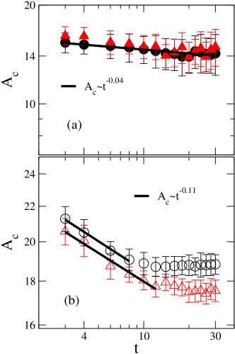
Figure 14: (Color online) Time evolution of the average area of crosssection A_c of the sampled dots with time for (a) the unrotated case, and (b) the rotated case. Symbols: open and closed circle (triangle) symbols denote data obtained with and without substrate rotation respectively, for Ar-GaAs (Ne-Si).

These results indicate that while no new dots are created with rotation (for $\theta>$ 0^∘), the uniformity of the density of the existing dots and the stability of the dot height are greatly enhanced with substrate rotation. Our results of the analysis of the dots are in agreement with previous experiments on dots obtained from normal incidence sputtering of semiconductors (Si), Gago et al. (2001) semiconductor alloys (GaSb, InSb); Facsko et al. (1999, 2001) as well as oblique incidence dots obtained from simultaneous sputtering and sample rotation (InP). Frost et al. (2000) In these experiments, the dot height has been reported to increase with time; and the average dot size have been reported to become constant with time.

To summarize, we have implemented substrate rotation for a solid-on-solid model of surface sputtering and used it to study the effects of concurrent rotation on the different possible topographies. In particular, we have studied the effect of rotation on the dot region as well as a detailed analysis of the time evolution of the dot characteristics (number, cross sectional area, and height) with and without substrate rotation. We found that different materials whose sputtering parameters fall within this region exhibit the same scaling behavior. The number of dots $N_{c}$ formed in the absence of substrate rotation decrease with time as $N_{c}\sim t^{-0.58}$, whereas $N_{c}$ is roughly constant with substrate rotation. Both with and without rotation the dot cross section $A$ finally becomes independent of time, however, it initially decreases according to $A\sim t^{-0.11}$ with rotation.

Additionally, for other choices of the sputtering conditions, we find different patterns which have not been observed experimentally so far. In particular we found transitions in time from one kind of surface structures (e.g. smooth, or holes) to other structures (like non-oriented structures), which can be explained only by the presence of non-linear effects. Hence, more sputtering experiments with different ion/substrate types and varying parameters are needed to verify whether the structures we predict by simulations can indeed be found experimentally.