Collective Oscillations in Classical Nonlinear Response of a Chaotic System

Abstract

We consider classical response in a strongly chaotic (mixing) system. As opposed to the case of stable dynamics, the nonlinear classical response in a chaotic system vanishes at large times. The physical behavior of the nonlinear response is attributed to the exponential time dependence of the stability matrix. The response also reveals certain features of collective resonances which do not correspond to any periodic classical trajectories. We calculate analytically linear and second-order response in a simple chaotic system and argue on the relevance of the model for interpretation of spectroscopic data.

Time-domain femtosecond spectroscopy constitutes a powerful tool that probes electronic and vibrational coherent dynamics of complex molecular systems in condensed phase TokmakoffetalPRL ; ZanniHochstrPNAS ; Fayer01 ; Jonas03 ; StolowJonas . Spectroscopic signals are directly related to optical response functions that carry detailed information on the underlying dynamical phenomena. At room temperatures the complexity often originates from slow strongly anharmonic vibrational modes that can be treated within the framework of classical mechanics.

A number of studies have been devoted to the classical response in stable (integrable) dynamical systems LeegwaterMukamel95 ; NEL04 ; KryvohuzCaoPRL05 . The nonlinear response functions have been shown diverge linearly with time, while the divergence can be eliminated by invoking a fully quantum description NEL04 ; KryvohuzCaoPRL05 . Although integrable dynamics represents only an approximation for realistic physical situations, weak deviations from the integrability do not eliminate the unphysical behavior of the response functions. This follows from the fact that the divergence is related to quasiperiodic motions on invariant tori KryvohuzCaoPRL05 . According to the Kolmogorov-Arnold-Moser (KAM) theory, most the invariant tori are not destroyed by small perturbations that break down integrability Arnold . Yet, stable dynamics would be typical for a close to equilibrium situation. At larger energies a generic situation would correspond to dynamical behavior with chaotic features Gutzwiller . Moreover, unstable (hyperbolic) dynamics may be more common due to the stability of chaos with respect to perturbations. It has been argued based on results of numerical analysis DellagoMukamel03 that chaotic dynamics appears to observe the convergence of the classical response functions. In spite of apparent importance, and to the best of our knowledge the problem of the nonlinear response in strongly chaotic systems has never been addressed using analytical methods. We note that analytical calculations of the response are rarely feasible in nonintegrable systems, whereas numerical simulations of chaotic dynamics are complicated by the exponential divergence of stability matrices DellagoMukamel03 .

In this Letter we show that (i) the classical response of the chaotic system exhibits decay and oscillations as a function of times between probing pulses, and (ii) the Fourier transform of $2D$ second order response function reveals broad and asymmetric peaks as signatures of chaos. This is the main result or our study.

A strongly chaotic (mixing) system is characterized by a special spectrum of the Liouville operator Ruelle86 ; RobertsMuz . The spectrum consists of complex Ruelle-Pollicott (RP) resonances that determine the asymptotic oscillations and decay of the correlations. This yields the linear response function directly related to the two-point correlation functions, in agreement with the fluctuation dissipation theorem (FDT). Nonlinear response, however, turns out to be more involved still with the noticeable effect of the resonances.

A system driven by a time-dependent external field ${\cal E}(t)$ is described by the Hamiltonian $H_{T}=H-f{\cal E}(t)$ with the the function $f(\bm{\eta})$ in phase space representing the dipole (see, e.g. Ref. DellagoMukamel03, ). The response functions $S^{(n)}$ that depend on $n$ time intervals describe the expansion of the measured signal $\langle f(\bm{\eta}(t))\rangle=\int d\bm{\eta}\,\rho f$ in a functional series in ${\cal E}$. The second-order response function reads

$$S^{(2)}(t_{1},t_{2})=\partial_{t_{1}}\int d{\bm{\eta}}fe^{-\hat{L}t_{2}}\left\{f,e^{-\hat{L}t_{1}}f\partial_{E}\rho_{0}\right\}.$$ (1)

where $\rho_{0}$ is the equilibrium distribution and $\hat{L}=\left\{H,\cdot\right\}$ is the Liouville operator of the unperturbed system.

A schematic picture of second-order response formation in a chaotic system that employs the Liouville phase space evolution is shown in Fig. 1.

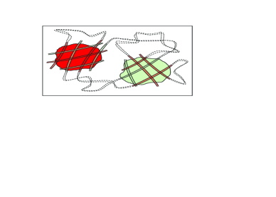
Figure 1: Schematic cross-section of the phase space along the surface given by the stable and unstable directions. Initial distribution of $f$ is presented by two regions $+$ and $-$ (dark red and light green). As time elapses the distribution elongates along unstable direction and contracts along stable one.

Propagating the observable $f$ in Eq. (1) backward in time we interpret the second-order response as an overlap of the distributions $f_{-}({\bm{\eta}})=\exp(\hat{L}t_{2})f$ and $\xi^{j}\partial_{j}f_{+}({\bm{\eta}})$ with $f_{+}=\exp(-\hat{L}t_{1})f\partial_{E}\rho_{0}$ and the vector field $\xi^{j}\partial_{j}=\{f,\cdot\}$. Since $\int d{\bm{x}}f=0$, we can for simplicity represent the function $f$ by two separate regions in the phase space where it adopts positive and negative values. In the case of hyperbolic dynamics evolution during time $t$ changes the regions’ shapes. For $|t|\gg 1$, the shape becomes similar to ribbon-like fettuccine: elongated along the unstable direction by a factor $\sim e^{\lambda t}$, narrowed along the stable one $\sim e^{-\lambda t}$ (with $\lambda$ being the Lyapunov exponent) and unchanged along the flow. Since $f_{-}$ results from reverse dynamics, the distributions $f_{+}$ and $f_{-}$ are elongated along the unstable and stable directions, respectively. Therefore, the overlap is represented by a large set of $N\sim e^{\lambda(t_{1}+t_{2})}$ small disconnected regions with the volume $v\sim e^{-\lambda(t_{1}+t_{2})}$. Since $f$ is represented by a positive and negative regions, the distribution $f_{-}$ consists of two positively and negatively ”charged” fettuccine and the cancellations result in a signal determined by a typical fluctuation proportional to $\sqrt{N}$, and the overlap integral attains a factor $\sqrt{N}v\sim e^{-\lambda(t_{1}+t_{2})/2}$ that turns out to be exponentially small. Yet, this is not the end of the story since the derivative $\xi^{j}\partial_{j}$ of a sharp feature along the stable direction can create exponentially large $\sim e^{\lambda t_{1}}$ factors. This is the Liouville space signature of the exponentially growing components of the stability matrix, which affects the response starting with second order due to FDTMKC96 ; DellagoMukamel03 . However, the divergent terms cancel out: decomposing ${\bm{\xi}}=\bm{\xi}_{0}+\bm{\xi}_{+}+\bm{\xi}_{-}$ into the direction along the flow, and unstable and stable components, we note that only the last term is potentially dangerous. Calculating the dangerous component of the overlap integral by parts we arrive at two contributions: the overlap of $\xi_{-}^{j}\partial_{j}f_{-}$ with $f_{+}$, and the overlap of $f_{-}$ with $f_{+}$ weighted with ${\rm div}{\bm{\xi}}_{-}$. The first contribution contains an additional $e^{-\lambda t_{2}}$ factor, the second one provides an additional factor independent of time. This results in a physical $\sim\exp^{-\lambda(t_{1}+t_{2})/2}$ large time asymptotics of the nonlinear response function.

Trajectories of a particle in arbitrary potential $U({\bm{r}})$ are known to be the same as for a free motion in a curved space with the metric $g_{ik}=(1-U({\bm{r}})/E)\delta_{ik}$ Arnold ; Gutzwiller . Although the potential generates nonuniform motion along the trajectories, one can expect chaotic behavior due to the exponentially growing separation between the trajectories. In addition, when the motion is finite, the accessible part of the configurational space at a given energy can be multiply connected. In the simplest case of two coordinates the motion occurs inside a disk-like region punctured by $g$ forbidden islands. Some fraction of trajectories approaches the boundaries so close that this can be qualified as reflection. Utilizing the original argument of Sinai Sinai reflection can be interpreted as continuing motion on the antipode replica of the accessible region glued to its original counterpart via the boundaries (see Appendix A and Ref. Arnold, ). The resulting compact surface has topology of a sphere with $g$ handles (Riemann surface of genus $g$). In the $g>1$ case the average curvature is negative, which results in unstable (hyperbolic) dynamics.

To rationalize the described above qualitative picture of response in a chaotic system we calculate the linear and second-order classical response functions for free motion in a Riemann surface $M^{2}$ of constant negative (Gaussian) curvature. This model that allows an exact solution has been serving as a prototype of classical chaos, as well as an example of semiclassical quantization Arnold ; Gutzwiller ; BalazsVoros .

The classical free-particle Hamiltonian

$$H({\bm{x}},\zeta)=(1/2m)g^{ik}p_{i}p_{k}=\zeta^{2}/2m\,,$$ (2)

depends on the absolute momentum value $\zeta$ only, and ${\bm{x}}\in M^{3}$ includes the two coordinates and momentum direction angle $\theta$. Therefore, the smooth compact $3D$ manifold $M^{3}$, which represents the subspace of phase space with fixed energy, is preserved in classical dynamics. Hereafter, we will use dimensionless units so that $m=1$ the curvature $K=-1$, and $\zeta=1$ (when energy is fixed). Our model allows for an exact solution due to strong Dynamical Symmetry (DS). To describe DS we adopt an agreement used in differential geometry by identifying a first-order differential operator of differentiating along the vector field with the vector field itself. We denote by $\sigma_{1}$ the vector field that describes the phase space dynamics, and set $\sigma_{z}=\partial/\partial\theta$, $\sigma_{2}=[\sigma_{1},\sigma_{z}]$. A simple local calculation yields $[\sigma_{2},\sigma_{z}]=-\sigma_{1}$ and $[\sigma_{1},\sigma_{2}]=-K\sigma_{z}$ which implies that in the constant negative curvature case the vector fields $\sigma_{z}$, $\sigma_{1}$, and $\sigma_{2}=[\sigma_{1},\sigma_{z}]$ form the Lie algebra $so(2,1)$. The group $SO(2,1)$ action in the reduced phase space $M^{3}$ is obtained by integrating of the $so(2,1)$ algebra action. DS with respect to the action of the group $G\cong SO(2,1)$ does not mean symmetry in a usual sense, i.e. that the system dynamics commutes with the group action, but rather reflects the fact that the Poisson bracket is given by a bi-vector field

$$\omega=\partial_{\zeta}\otimes\sigma_{1}-\sigma_{1}\otimes\partial_{\zeta}+\zeta^{-1}\left(\sigma_{2}\otimes\sigma_{z}-\sigma_{z}\otimes\sigma_{2}\right)\,.$$ (3)

In particular, the vector field that determines classical dynamics is given by an element $\sigma_{1}$ of the corresponding Lie algebra $so(2,1)$, whereas the stable and unstable directions are determined by $\sigma_{z}\mp\sigma_{2}$.

DS implies that the space of phase-space distributions constitutes a representation of $SO(2,1)$ and, being decomposed into a sum of irreducible representations, provides a set of uncoupled evolutions. Unitary irreducible representation of $SO(2,1)$ are well-known and can be conveniently implemented in terms of functions $\Psi(u)$ in a circle Lang . Principal series representations relevant for our calculations are labeled by imaginary parameter $s$ with the Liouville operator $\sigma_{1}=\sin u\partial_{u}+(1/2-s)\cos u$. The aforementioned decomposition identifies the angular harmonic $\Psi_{k}(u)=e^{iku}$ in a circle with a phase-space distribution $\psi_{k}(\bm{x};s)$ with given angular momentum $\sigma_{z}\psi_{k}({\bm{x}};s)=ik\psi_{k}({\bm{x}};s)$. Commutation law in $so(2,1)$ entails $\sigma_{\pm}\psi_{k}({\bm{x}};s)=(\pm k+1/2-s)\psi_{k\pm 1}({\bm{x}};s)$ with two anti-Hermitian conjugated ladder operators $\sigma_{\pm}=\sigma_{1}\pm i\sigma_{2}$, $\sigma_{\pm}^{\dagger}=\sigma_{\mp}$. Any relevant distribution can be decomposed in the modes $\psi_{k}({\bm{x}};s)$, where $s$ adopts discrete values (the spectrum). The spectrum $\{s_{\alpha}\}$ can be related to the eigenvalues of the Laplacian operator in $M^{2}$ by identifying $\nabla^{2}=-\frac{1}{2}(\sigma_{+}\sigma_{-}+\sigma_{-}\sigma_{+})$ and $-\nabla^{2}\psi_{0}({\bm{x}};s)=(1/4-s^{2})\psi_{0}({\bm{x}};s)$.

The dipole $f$ is a function in $M^{2}$, i.e. a function in phase space that does not depend on both $\zeta$ and momentum direction $\theta$, hence $\sigma_{z}f=0$, and $f$ can be expanded as a sum over the principal series representations $f=\sum_{s}B_{s}\psi_{0}(\bm{x};s)$.

The integrands in the response function (1) include the result of action of the evolution operator $e^{-\hat{L}t}$ on the components $\psi_{0}(\bm{x};s)$ of the dipole momentum and their derivatives resulting from the Poisson brackets. To simplify the calculations, we transform the expressions of response functions in a way that the evolution of derivatives of $\psi_{0}(\bm{x};s)$ does not appear.

We use the representation in the circle to find the expansion of $e^{-\hat{L}t}\psi_{0}(\bm{x};s)$ over basis vectors $\psi_{k}({\bm{x}};s)$,

$$e^{-\hat{L}t}\psi_{0}(\bm{x};s)=\sum\limits_{k=-\infty}^{+\infty}A_{k}(t;s)\psi_{k}(\bm{x};s)\,.$$ (4)

Since $e^{-\hat{L}t}\Psi_{0}(u)$ represents a function obtained as the result of the action of the evolution operator on $\Psi_{0}(u)\equiv 1$, it can be found by solving the equation $\partial_{t}g(t,u)+\hat{L}g(t,u)=0$ supplemented with initial condition $g(0,u)=1$. In the principal series representation with $\mathrm{Re}\,s=0$, $\mathrm{Im}\,s>0$, and the equation takes the following form:

$$\partial_{t}g(t,u)+\left(\sin u\partial_{u}+(1/2-s)\cos u\right)g(t,u)=0\,.$$ (5)

The solution can be easily found, and thus after the integration $\int du\,e^{-iku}g(t,u)$ we obtain $A_{k}(t;s)$:

$$A_{k}(t;s)=\frac{2(-1)^{k}\left(1-e^{-2t}\right)^{k}\Gamma(k+1/2-s)}{\sqrt{\pi}\Gamma(1/2-s)}e^{-t/2}\times$$

$${\rm Re}\left[\frac{\Gamma(s)e^{st}}{\Gamma(k+\frac{1}{2}+s)}\,_{2}F_{1}\left(k+\frac{1}{2}-s,k+\frac{1}{2},1-s,e^{-2t}\right)\right],$$

where ${}_{2}F_{1}$ is the Gauss hypergeometric function. For details see Appendix B and Ref. tobe, .

The linear response function can be obviously expressed via $A_{0}(t;s)$. The calculation involves only the first part of the Poisson bracket, and the result is conveniently represented similarly to the fluctuation-dissipation relation $S^{(1)}(t)\propto\partial_{t}A_{0}(t;s)$ MKC96 .

For large $t$ the linear response function shows damped oscillations $e^{(\pm s-1/2)t}$. The expansion in powers of $e^{-2t}$ corresponds to RP resonances RobertsMuz . Only even RP resonances contribute to the response function. The expansion is a converging series in $e^{-2t}$ if $e^{-2t}<1$, i.e. $t>0$. Since the dipole $f(\bm{x})$ can decomposed in irreducible representations characterized by different values of $s$, the linear response function constitutes a linear combination of contributions with coefficients $B_{s}^{2}$.

The second-order response function can be calculated using Eqs. (1) and (3) tobe . The calculation can be substantially simplified by propagating the observable $f$ in Eq. (1) backwards in time and making use of $\left(e^{-\hat{L}t_{2}}\right)^{\dagger}=e^{\hat{L}t_{2}}$. Then we apply Eq. (4) to decompose $e^{\hat{L}t_{2}}\psi_{0}(\bm{x};s)$ in $\psi_{k}(\bm{x};s)$ and $e^{-\hat{L}t_{1}}\psi_{0}(\bm{x};s)$ in $\psi_{l}(\bm{x};s)$. The integration over the reduced phase space includes an integral over the momentum direction $\theta$ that results in vanishing of all terms with $k\neq l\pm 1$. The second order response function consists of several contributions, $S^{(2)}=\sum_{j}\sum\limits_{p,q,r}B_{p}B_{q}B_{r}\sum_{k=0}^{\infty}(-1)^{k}S^{(2)}_{j,k}$ of similar form, e.g.:

$$S^{(2)}_{1,k}=(-1)^{k}k\left(k+\frac{1}{2}-p\right)a^{pqr}_{k}A_{k+1}^{*}(t_{2};p)\frac{\partial A_{k}(t_{1};r)}{\partial t_{1}},$$

with the matrix elements

$$a^{s_{1}s_{2}s_{3}}_{k}=\int d\bm{x}\,\psi_{k}^{*}(\bm{x};s_{1})\psi_{0}(\bm{x};s_{2})\psi_{k}(\bm{x};s_{3})\,.$$ (6)

We further establish recurrent relations for coefficients (6) that allow expressing all of them via few “initial conditions”, e.g. $a^{s_{1}s_{2}s_{3}}_{0}$. For instance, in the simplest case $s_{1}=s_{2}=s_{3}=s$, the recurrent relations read $a_{k+1}=\frac{8k^{2}+1-s^{2}}{(2k+1)^{2}-s^{2}}a_{k}-\frac{(2k-1)^{2}-s^{2}}{(2k+1)^{2}-s^{2}}a_{k-1}$, and all coefficients $a_{k}$ are expressed via $a_{0}$ due to the symmetry $a_{k}=a_{-k}$ tobe . In this case we find the asymptotic behavior $a_{k}\propto k^{-1/2\pm s}$ for $k\to\infty$. The summation over $k$ is performed numerically. The set of coefficients $a_{0}$, as well as the spectrum $\{s_{\alpha}\}$ are attributes of a particular Riemann surface. Constant curvature Riemann surfaces of genus $g$ are classified by the so-called moduli spaces whose dimensions grow linearly in $g$. Therefore, any finite set $s_{\alpha}$ of spectral elements, as well as the relevant set of coefficients $a_{0}$ can be implemented for some particular Riemann surface, and hereafter we will treat them as independent parameters.

The convergence of the series over $k$ is ensured by the dependence $A_{k}(t;s)\propto\exp(-2ke^{-t})$ for large $k$. The series is almost sign-alternating, and the dependence of the summand magnitude on $k$ becomes smoother with increasing $k$, independently of $t$. This allows for an effective procedure that evaluates the series, since it does not involve numerical summation of the exponentially increasing with $t$ number of terms. The procedure also works in any order of $e^{-t_{1}}$ and $e^{-t_{2}}$ obtained from the hypergeometric expansions of $A_{k}(t;s)$ tobe . In Ref. tobe2, we extend our study of optical response by adding Langevin noise to classical deterministic dynamics. We identify the RP resonances as the eigenvalues of the related Fokker-Planck operator $\hat{{\cal L}}=-\kappa\nabla^{2}+\hat{L}$ in the weak-noise limit $\kappa\to 0$. We demonstrate that a standard spectral decomposition of the response functions in the eigenmodes of the Fokker-Planck operator $\hat{{\cal L}}$ has a well-defined limit at $\kappa\to 0$ that reproduces our expression for the classical response functions.

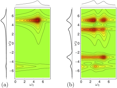
Figure 2: Absolute value of $2D$ Fourier transform of the second order response function: (a) single resonance $s=5i$, (b) linear combination of terms with two resonances $s_{1}=3i$ and $s_{2}=5i$. Linear plots show cross-sections of the spectra at $\omega_{1}=\omega_{2}=5$.

The absolute value of the $2D$ Fourier transform of the second-order response function presented in Fig. 2 shows diagonal and cross peaks, as well as a stretched along the $\omega_{1}$ direction feature (real and imaginary parts are presented in Appendix C). The latter originates from time-domain damped oscillations with variable period and can be interpreted as a signature of chaos (instability) in the underlying dynamics. Also note that in our chaotic case the peak frequencies may not be attributed to any particular periodic motions, although they can be expressed in terms of all periodic orbits via the dynamical $\zeta$-function Ruelle86 . Therefore, they can be referred to as collective chaotic resonances.

Our results can be applied to the interpretation of spectroscopic data. Classical chaos is quite generic for dynamics in large molecules and molecular networks coupled via hydrogen bonds. Even for a small number of vibrational modes, e.g. in small systems of hydrogen bonds Hbonds , the shape of the effective potential energy can lead to chaotic dynamics. Moreover, the chaos may be caused by just some regions with nonuniform curvature of the potential surface Pettini .

In the present Letter we studied classical nonlinear response in a strongly chaotic (mixing) system. Detailed analysis performed for free motion in a Riemann compact surface of constant negative curvature demonstrated that calculation of the response based on Liouville space dynamics does not have fundamental difficulties. We demonstrated that peaks in $2D$ spectra are not necessarily attributed to periodic or quasiperiodic motions, but rather can have collective nature. We argue that collective resonances should be accompanied by stretched features in $2D$ spectra that constitute a spectroscopic signature of underlying dynamical chaos.

Appendix A Effective negative curvature of configuration space

In this appendix we rationalize a close qualitative connection between classical dynamics of multidimensional motion in a potential with forbidden islands and a geodesic flow in a compact manifold with non-trivial topology. For the sake of simplicity we consider the case of two coordinates. The motion is restricted to a disk-like region punctured by forbidden islands. Boundaries of the accessible region correspond to the lines where the total energy coincides with the potential energy. To employ the original argument of Sinai Sinai we glue the accessible region of the configuration space to its antipode replica along the boundary. A reflection from the boundary can be thought of as continuing motion in the other component. The resulting surface is compact and its topology is characterized by genus $g$ (the number of handles attached to a sphere) corresponding to the number of original islands.

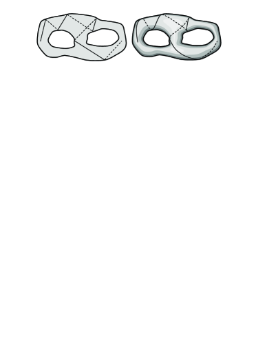
Figure 3: Motion in the multiply connected flat configuration space is equivalent to motion on the curved surface. Idealization of the hard-wall potential: Trajectories are confined within the original classically accessible $2D$ configuration space reflecting on its boundaries (left). Reflections can be viewed as transitions to the antipode surface component glued to the original one along the boundaries (right). Trajectories on the deformed smooth version of the resulting compact surface are shown as solid and dashed lines, which correspond to the original and antipode components, respectively.

In Fig. 3 we show both the original billiard-like motion in the configuration space and the equivalent motion in two components assembled together that form a compact surface of genus $g=2$. As mentioned in the main text trajectories of a particle moving in a potential resemble the geodesic lines in curved space with the metric $g_{ik}=(1-U({\bm{r}})/E)\delta_{ik}$. The regions of the configuration space that correspond to negative curvature work as a defocusing lenses, causing instability (divergence of close trajectories). For example, close trajectories diverge every time they approach the boundary of the classically inaccessible island or pass a region of a potential local maximum that belongs to the accessible region. Passing through the stable regions with positive curvature cannot compensate for the instability, since stability reflects oscillatory, rather than converging features in the dynamics of the trajectory deviation. In particular, existence of unstable regions combined with ergodicity ensures exponential divergence of trajectories over long enough times. According to the Gauss-Bonnet theorem, in the $g>1$ case the average curvature is negative, which implies regions of instability.

Appendix B Liouville-space calculation of response functions

Response functions can be obtained starting with the driven Liouville equation $\partial_{t}\rho+\hat{\cal L}={\cal E}(t)\{f,\rho\}$. The phase space distribution $\rho(\bm{\eta},t)$ is represented as a functional series in ${\cal E}(t)$ with the initial distribution $\rho_{0}$ being the zero-order contribution. In our case of interest the observable coincides with the dipole moment $f$ that represents coupling to the probe field. The linear and second-order classical response functions are expressed via the Poisson brackets as

$$S^{(1)}(t) =\int d{\bm{\eta}}\,f({\bm{\eta}})e^{-\hat{L}t}\{f({\bm{\eta}}),\rho_{0}\}\,,$$ (7)

$$S^{(2)}(t_{1},t_{2}) =\int d{\bm{\eta}}\,f({\bm{\eta}})e^{-\hat{L}t_{2}}\{f({\bm{\eta}}),e^{-\hat{L}t_{1}}\{f({\bm{\eta}}),\rho_{0}\}\}\,.$$

We start with utilizing the fact that the equilibrium distribution $\rho_{0}$ depends on energy $E=\zeta^{2}/2$ only, and make a transformation based on the FDT. This brings us to Eq. (1).

The problem of free motion in a compact surface of constant negative curvature possesses dynamical $SO(2,1)$ symmetry. DS means that the flow is determined by the $so(2,1)$ generator $\sigma_{1}$, it also conserves the stable and unstable directions; this is expressed by the relation $e^{\sigma_{1}t}(\sigma_{2}\pm\sigma_{z})=e^{\pm t}(\sigma_{2}\pm\sigma_{z})e^{\sigma_{1}t}$.

Any phase-space distribution can be decomposed into a direct sum of irreducible representations; only principal series representations of $SO(2,1)$ contribute to the linear and second-order response tobe . DS implies that the distributions in different representations evolve independently. Distributions in irreducible representation can be implemented as functions in a circle with the basis of angular harmonics $\Psi_{k}(u)=e^{iku}$. The evolution in the circle is determined by Eq. (5) that, given the initial condition $g(0,u)=\Psi(u)\equiv 1$, can be solved using the method of characteristics:

$$g(t,u)=\left(\cosh t+\sinh t\cos u\right)^{s-\frac{1}{2}}\,.$$

Implementing the correspondence of natural scalar products in $M^{3}$ and in the circle, we find the expansion coefficients in Eq. (4)

$$A_{k}(t;s)=\int\limits_{0}^{2\pi}\frac{du}{2\pi}e^{-iku}g(t,u)\,.$$

These coefficients represent the main dynamical ingredient in the response function calculation. We represent them in terms of the hypergeometric functions. Alternative representations have been derived in the context of two-point correlationsBalazsVoros ; RobertsMuz . The linear response function is determined by the dynamical part alone:

$$S^{(1)}(t)=\frac{\partial}{\partial t}\int\limits_{0}^{\infty}d\zeta\,A_{0}(\zeta t;s)\frac{\partial\rho_{0}}{\partial\zeta}\,.$$

Calculation of the second-order response function is more involved. Substituting the Poisson brackets (3) into Eq. (7) the $2D$ signal adopts a form

$$S^{(2)}(t_{1},t_{2})=\frac{\partial}{\partial t_{1}}\int d{\bm{x}}\,d\zeta\,\times$$

$$\left\{\zeta t_{2}\left(\sigma_{1}e^{\sigma_{1}\zeta t_{2}}f\right)^{*}(\sigma_{1}f)(e^{-\sigma_{1}\zeta t_{1}}f)\right.$$

$$+\left(e^{\sigma_{1}\zeta t_{2}}f\right)^{*}(\sigma_{1}f)(e^{-\sigma_{1}\zeta t_{1}}f)$$

$$\left.+\left(e^{\sigma_{1}\zeta t_{2}}f\right)^{*}(\sigma_{2}f)(\sigma_{z}e^{-\sigma_{1}\zeta t_{1}}f)\right\}\frac{\partial\rho_{0}}{\partial\zeta}\,.$$

All terms in parentheses are further expanded in irreducible representations and angular harmonics. The resulting contributions include two coefficients $A_{k}$ and a triple product given by Eq. (6). The latter is the geometrical ingredient that appears in nonlinear response functions. The simplest expression for the second-order response function that incorporates different collective resonances, originates from two terms in the decomposition $f=B_{s_{1}}\psi_{0}(\bm{x};s_{1})+B_{s_{2}}\psi_{0}(\bm{x};s_{2})$. Then the response function reads

$$S^{(2)}=\int d\zeta\frac{\partial\rho_{0}}{\partial E}\frac{\partial}{\partial t_{1}}\sum\limits_{p,q,r=s_{1},s_{2}}B_{p}B_{q}B_{r}\sum\limits_{n=0}^{\infty}(-1)^{n}\times$$

$$\Biggl{\{}\biggl{[}\biggl{(}n+\frac{1}{2}+r\biggr{)}a^{pqr}_{n}-\biggl{(}n+\frac{1}{2}+p\biggr{)}a^{pqr}_{n+1}\biggr{]}\times$$

$$\biggl{[}t_{2}\frac{\partial}{\partial t_{2}}-n\biggr{]}(A_{n}^{*}(t_{2};p)A_{n+1}(t_{1};r))$$

$$-\biggl{[}\biggl{(}n+\frac{1}{2}-p\biggr{)}a^{pqr}_{n}-\biggl{(}n+\frac{1}{2}-r\biggr{)}a^{pqr}_{n+1}\biggr{]}\times$$

$$\biggl{[}t_{2}\frac{\partial}{\partial t_{2}}+n+1\biggr{]}(A_{n+1}^{*}(t_{2};p)A_{n}(t_{1};r))\Biggr{\}}\,.$$

It turns out that the resulting second-order response function may be represented as a double expansion over RP resonances. The expansion is nontrivial: one encounters diverging series if the expansion of quantities $A_{n}(t;s)$ is performed first. Fortunately, we have found an efficient scheme for numerical evaluation of the seriestobe . The procedure also demonstrates that the second-order response is indeed expanded in the RP resonances.

Appendix C 2D spectra for spectroscopy of a chaotic system

In this appendix we present some details on $2D$ spectra that characterize the second-order response of a chaotic dynamical system considered in this Letter. Experimental data on $2D$ time-domain spectroscopy that probes the response function $S^{(2)}(t_{1},t_{2})$ is usually presented using the so-called $2D$ spectra that constitute a numerical $2D$ Fourier transform of the response function with respect to $t_{1}$ and $t_{2}$. The absolute value of the $2D$ spectra for our dynamical system are given in Fig. 2, whereas in Fig. 4 we present the real and imaginary parts.

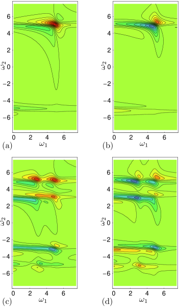
Figure 4: Real and imaginary parts of $2D$ spectra: (a) real part, (b) imaginary part with the single resonance $s=5i$; (c) real part, (d) imaginary part of linear combination of terms with two different resonances $s_{1}=3i$ and $s_{2}=5i$.

As follows from the general picture presented in the main text, for a given unperturbed dynamics the response function depends on the expansion of the dipole function $f$ in the eigenmodes of the Laplace operator: each eigenmode provides with an oscillation in the signal. Since the dipole is generally a smooth function of the system coordinates, the number of eigenmodes that participate in the expansion is typically small. To study the important features of the signals we consider the cases of one and two oscillation in the signal. In the first case we see a diagonal peak with a stretched feature along $\omega_{1}$ direction; such stretching never occurs due to a periodic orbit in an integrable system even if it is coupled to a harmonic bath. In the second case we see both diagonal and cross peaks accompanied by the stretched features.

References

- (1) A. Tokmakoff, M. J. Lang, D. S. Larsen, G. R. Fleming, V. Chernyak, and S. Mukamel, Phys. Rev. Lett. 79, 2702 (1997).
- (2) M. C. Asplund, M. T. Zanni, and R. M. Hochstrasser, Proc. Natl. Acad. Sci. USA 97, 8219 (2000).
- (3) M. D. Fayer, Ann. Rev. Phys. Chem. 52, 315 (2001).
- (4) D. M. Jonas, Ann. Rev. Phys. Chem. 54, 425 (2003).
- (5) A. Stolow and D. M. Jonas, Sciense 305, 1575 (2004).
- (6) J. A. Leegwater and S. Mukamel, J. Chem. Phys. 102, 2365 (1995).
- (7) W. G. Noid, G. S. Ezra, and R. F. Loring, J. Phys. Chem. B 108, 6536 (2004).
- (8) M. Kryvohuz and J. Cao, Phys. Rev. Lett. 95, 180405 (2005); 96, 030403 (2006); J. Chem. Phys.122, 024109 (2005).
- (9) M. C. Gutzwiller, Chaos in Classical and Quantum Mechanics, Springer Verlag, 1990.
- (10) V. I. Arnold, Mathematical Methods of Classical Mechanics, Springer Verlag, 1989.
- (11) N. L. Balazs and A. Voros, Phys. Rep. 143, 109 (1986).
- (12) Y. G. Sinai, Russ. Math. Surv. 25, 137 (1970).
- (13) C. Dellago and S. Mukamel, Phys. Rev. E 67, 035205(R) (2003); J. Chem. Phys. 119, 9344 (2003).
- (14) D. Ruelle, Phys. Rev. Lett. 56, 405 (1986).
- (15) S. Roberts and B. Muzykantskii, J. Phys. A: Math. Gen. 33, 8953 (2000).
- (16) S. Mukamel, V. Khidekel, and V. Chernyak, Phys. Rev. E 53, R1 (1996).
- (17) P. C. Martin, Mesurements and correlation functions (Gordon and Breach, New York, 1968).
- (18) A. A. Kirillov, Elements of the Theory of Representation of Groups, Springer Verlag, 1986.
- (19) S. Lang, , Addison-Wesley, 1975.
- (20) F. L. Williams, Lectures on the Spectrum of .
- (21) S. V. Malinin and V. Y. Chernyak, to be published.
- (22) S. V. Malinin and V. Y. Chernyak, to be published.
- (23) J. D. Eaves, J. J. Loparo, C. J. Fecko, S. T. Roberts, A. Tokmakoff, and P. L. Geissler, Proc. Natl. Acad. Sci. USA 102, 13019 (2005).
- (24) L. Casetti, C. Clementi, and M. Pettini, Phys. Rev. E 54, 5969 (1996).