One-particle dynamical correlations in the one-dimensional Bose gas

Abstract

The momentum- and frequency-dependent one-body correlation function of the one-dimensional interacting Bose gas (Lieb-Liniger model) in the repulsive regime is studied using the Algebraic Bethe Ansatz and numerics. We first provide a determinant representation for the field form factor which is well-adapted to numerical evaluation. The correlation function is then reconstructed to high accuracy for systems with finite but large numbers of particles, for a wide range of values of the interaction parameter. Our results are extensively discussed, in particular their specialization to the static case.

1 Introduction

For many decades now, there has been a sustained interest in the physics of one-dimensional quantum systems, in no small part due to Bethe’s fundamental paper on the Heisenberg spin chain [1]. This publication laid the foundation for what has today become one of the most important fields of mathematical physics, namely the theory of Bethe Ansatz integrable models.

More recently, renewed motivation for the study of interacting quantum models in 1D has come from their growing number of experimental realizations. The simplest system to consider is probably the one-dimensional gas of bosons with local (delta function) interaction (known as the Lieb-Liniger model [2]), which can effectively describe atoms confined using optical lattices [3, 4, 5, 6, 7, 8, 9, 10, 11]. A wide range of interactions are accessible, even the strongly-interacting (free fermion-like) limit considered long ago by Tonks and Girardeau [12, 13].

The integrability of the Lieb-Liniger model is by now textbook material [14, 15, 16, 17], and many of the standard methods now used in the field were in fact first developed and applied to it. For example, after the construction of the ground state and elementary excitations in [2], the Yang-Yang approach to thermodynamics was introduced in [18], leading the way to nonperturbative results on the equilibrium properties of the infinite system at arbitrary temperatures.

The motivation of the present paper is to help further our understanding of the interacting Bose gas in one dimension, by addressing one of the long-standing unresolved problems associated to it: the calculation of correlation functions. The importance of this is clear, in view of the fact that most experimentally-accessible response functions are expressible in terms of a few basic dynamical correlation functions of local physical fields.

Because of the relative complexity of the Bethe Ansatz eigenfunctions, it has proved much more difficult to provide information on correlation functions than on thermodynamics. For the interacting Bose gas, the first set of results probably dates back to the work of Girardeau [13], who considered the strongly-interacting limit. This represents a major simplification in that the spectrum becomes that of free fermions. The bosonic density operator then coincides with a free fermionic one, in view of its blindness to particle statistics. Handling particle statistics in the same limit allows to obtain the one-body density matrix as the determinant of a Fredholm integral operator, both at zero and nonzero temperatures [19, 20, 21, 22].

Away from the Tonks-Girardeau (TG) limit, static local moments of the density operator can be obtained. The second moment $g_{2}=\langle:n^{2}(x):\rangle$ is given directly from the derivative of the partition function with respect to the interaction parameter (the Hellmann-Feynman theorem) [23], but higher moments $g_{n}$ with $n>2$ are more challenging. These were computed for arbitrary temperature in a large coupling expansion in [24, 25, 26]. At zero temperature, the third moment $g_{3}$ was obtained exactly for any interaction in [27] using an integrable lattice regularization of the Lieb-Liniger model coupled with Conformal Field Theory [28, 29] considerations.

The full calculation of correlation functions beyond either the static of local cases remains analytically intractable to this day. Besides formulations for the asymptotics based on Conformal Field Theory, there exist important results providing determinant representations of the exact correlators in terms of auxiliary quantum fields, which ultimately map the infinite-volume problem to the calculation of the determinant of a Fredholm operator obeying a completely integrable integro-differential equation [30, 31, 32, 33, 34]. The asymptotics of the correlation functions can then be obtained by solving a Riemann-Hilbert problem (see [15] and references therein for an introduction to the subject). Closed-form analytical expressions for general correlation functions have however not yet been obtained.

Here, we make use of another strategy which one of us originally developed for dynamical spin-spin correlation functions in Heisenberg spin chains [35, 36]. Our objective is not to give final answers to the theoretical computation of correlation functions, but rather to provide a reliable and practical computational scheme for obtaining them to very high precision. This will be of great help for experimental comparisons (where finite resolutions are inevitable) or comparison with other theoretical methods. We specialize here to one-body correlations, following on our earlier work [37] on dynamical density-density correlations.

The overall strategy is summarized as follows: two-point correlation functions are expressed as an appropriate sum of form factors over intermediate states, and the summation is carried out numerically. The form factors of local operators are expressed as determinants of matrices whose entries are simple functions of the sets of Bethe rapidities of the two eigenstates involved (for the density, they were obtained in [38, 31]; see however the more practical representaion we offer here for the field form factor). The summation over intermediate states can itself be aggressively optimized by making use of the fact that not all intermediate states contribute equally to the desired correlator. Such an optimized method is in principle applicable to any integrable model as long as the determinant representations of the form factors are known, and was baptized the ABACUS method [39]. We here carry on with our study of the Lieb-Liniger model by providing the corresponding computations for its one-particle dynamical correlation function.

The plan of the paper is as follows. We first review the basic formulation of the theory, and define the correlations we will be interested in. The Algebraic Bethe Ansatz for the model is thereafter presented, and used to derive a simplified representation for the one-particle form factor in terms of the determinant of a single matrix. We then present the results for the correlation functions for a range of values of the interaction parameter, and discuss the results in detail, in particular their specialization to the static case (momentum distribution function and one-body density matrix). Conclusions and directions for future work are presented at the end.

2 Definitions

We consider a ring of length $L$, with $N$ bosonic particles interacting repulsively with each other through a local potential of strength $c$. The time evolution of this system is controlled by the Lieb-Liniger Hamiltonian [2]

$${\cal H}_{N}=-\sum_{j=1}^{N}\frac{\partial^{2}}{\partial x_{j}^{2}}+2c\sum_{1\leq j<l\leq N}\delta(x_{j}-x_{l}).$$ (1)

An alternate second-quantized formulation is obtained by introducing canonical Bose fields $\Psi(x)$ and $\Psi^{\dagger}(x)$ with equal-time commutation relations

$$\left[\Psi(x),\Psi^{\dagger}(y)\right]=\delta(x-y),\hskip 14.22636pt\left[\Psi(x),\Psi(y)\right]=\left[\Psi^{\dagger}(x),\Psi^{\dagger}(y)\right]=0.$$ (2)

The Fock vacuum $|0\rangle$ is then defined by

$$\Psi(x)|0\rangle=0,\hskip 14.22636pt\langle 0|\Psi^{\dagger}(x)=0,\hskip 14.22636pt\langle 0|0\rangle=1,$$ (3)

and thus the model corresponds to the quantum nonlinear Schrödinger equation,

$$H=\int_{0}^{L}dx\left[\partial_{x}\Psi^{\dagger}(x)\partial_{x}\Psi(x)+c\Psi^{\dagger}(x)\Psi^{\dagger}(x)\Psi(x)\Psi(x)\right].$$ (4)

The Bethe Ansatz provides a basis for the Fock space. More precisely, in the repulsive case $c>0$ which we are considering, each eigenfunction in the $N$-particle sector is fully described by a set of $N$ real parameters $\{\lambda\}_{N}$, solution to a set of coupled nonlinear equations (the Bethe equations, which we will review and discuss in more details in the next section).

Our aim here is to present computations of the zero temperature one-particle dynamical correlation function

$$G_{2}(x,t)\equiv\langle\Psi^{\dagger}(x,t)\Psi(0,0)\rangle_{N}$$ (5)

as a function of the interaction parameter $c$ (we consider here only the repulsive case $c>0$). By identifying the state $|\{\lambda\}\rangle$ with the ground state and using the closure relation of Bethe eigenstates, this correlation function can be represented as a sum over form factors of the local field operator between ground- and excited state as

$$G_{2}(x,t)=\sum_{\{\mu\}}\frac{\langle\{\lambda\}|\Psi^{\dagger}(x,t)|\{\mu\}\rangle\langle\{\mu\}|\Psi(0,0)|\{\lambda\}\rangle}{\langle\{\lambda\}|\{\lambda\}\rangle\langle\{\mu\}|\{\mu\}\rangle}.$$ (6)

The evaluation of this expression can be performed in three steps: first, finding the solution of the Bethe equations; second, computing the form factors; finally, performing the summation over intermediate states. We begin by providing a new representation for the form factors, using the Algebraic Bethe Ansatz, which allows all these steps to be efficiently implemented numerically for finite numbers of particles.

3 Algebraic Bethe Ansatz and Form Factors

The central object of the Algebraic Bethe Ansatz [40] (or Quantum Inverse Scattering Method; for an introduction to the concepts and terminology, see [15]) is the $R$-matrix, which solves the Yang-Baxter equation and takes the following form for the Lieb-Liniger model (quantum nonlinear Schrödinger equation):

$$R(\lambda,\mu)=\left(\begin{array}[]{cccc}f(\mu,\lambda)&0&0&0\\ 0&g(\mu,\lambda)&1&0\\ 0&1&g(\mu,\lambda)&0\\ 0&0&0&f(\mu,\lambda)\end{array}\right),$$ (11)

in which

$$g(\lambda,\mu)=\frac{ic}{\lambda-\mu},\hskip 14.22636ptf(\lambda,\mu)=\frac{\lambda-\mu+ic}{\lambda-\mu}.$$ (12)

Other standard functions which we will use later are defined as

$$h(\lambda,\mu)=\frac{\lambda-\mu+ic}{ic},\hskip 14.22636ptt(\lambda,\mu)=\frac{(ic)^{2}}{(\lambda-\mu)(\lambda-\mu+ic)}=\frac{g(\lambda,\mu)}{h(\lambda,\mu)}.$$ (13)

The monodromy matrix, which will be used to construct all the conserved charges (in particular, the Hamiltonian) is represented in auxiliary space as

$$T(\lambda)=\left(\begin{array}[]{cc}A(\lambda)&B(\lambda)\\ C(\lambda)&D(\lambda)\end{array}\right),$$ (16)

where the $A,B,C,D$ operators act in the Fock space as follows. The vacuum is an eigenvector of $A$ and $D$,

$$A(\lambda)|0\rangle=a(\lambda)|0\rangle,\hskip 14.22636ptD(\lambda)|0\rangle=d(\lambda)|0\rangle$$ (17)

with $a(\lambda)=e^{-iL\lambda/2}$ and $d(\lambda)=e^{iL\lambda/2}$, whereas $B$ and $C$ respectively act as raising and lowering operators with the annihilation properties

$$\langle 0|B(\lambda)=0,\hskip 14.22636ptC(\lambda)|0\rangle=0.$$ (18)

The commutation relations between these operators are quadratic, and given by

$$R(\lambda,\mu)(T(\lambda)\otimes T(\mu))=(T(\mu)\otimes T(\lambda))R(\lambda,\mu).$$ (19)

The Hamiltonian is related by trace identities to the trace of the monodromy matrix, $A(\lambda)+D(\lambda)$, and these can therefore be diagonalized simultaneously. The (unnormalized) eigenvectors of the Hamiltonian are constructed as

$$|\{\lambda\}_{N}\rangle=\prod_{j=1}^{N}B(\lambda_{j})|0\rangle,\hskip 14.22636pt\langle\{\lambda\}_{N}|=\langle 0|\prod_{j=1}^{N}C(\lambda_{j}),$$ (20)

provided that the rapidities are solution to the Bethe equations

$$e^{i\lambda_{j}L}=\prod_{l\neq j}\frac{\lambda_{j}-\lambda_{l}+ic}{\lambda_{j}-\lambda_{l}-ic},\hskip 14.22636ptj=1,...,N$$ (21)

or in logarithmic form,

$$\lambda_{j}+\frac{1}{L}\sum_{l=1}^{N}2~{}\mbox{arctan}\frac{\lambda_{j}-\lambda_{l}}{c}=\frac{2\pi}{L}I_{j},\hskip 14.22636ptj=1,...,N$$ (22)

where the quantum numbers $I_{j}$ are half-odd integers for $N$ even, and integers for $N$ odd. Proper eigenfunctions are obtained for sets of non-coincident rapidities $\lambda_{j}\neq\lambda_{l},j\neq l$. Since the left-hand side of (22) is a monotonous function of $\lambda_{j}$, it can be proven that all solutions are real [18]; we can moreover span the whole Fock space by choosing sets of ordered quantum numbers $I_{j}>I_{l},j>l$ meaning that $\lambda_{j}>\lambda_{l},j>l$.

Once the Bethe equations are solved for the rapidities, the eigenstate is fully characterized. The state norm is obtained from the Gaudin-Korepin formula [14, 41], which can be proven by making use of the commutation relations between $B$ and $C$ operators:

$$\langle\{\lambda\}_{N}|\{\lambda\}_{N}\rangle=c^{N}\prod_{j>k=1}^{N}\frac{\lambda_{jk}^{2}+c^{2}}{\lambda_{jk}^{2}}\mbox{det}_{N}{\cal G}(\{\lambda\})\equiv||\{\lambda\}_{N}||^{2}$$ (23)

in which ${\cal G}$ is the Gaudin matrix, whose entries are simple analytical functions of the rapidities,

$${\cal G}_{jk}(\{\lambda\}_{N})=\delta_{jk}\left[L+\sum_{l=1}^{N}K(\lambda_{j},\lambda_{l})\right]-K(\lambda_{j},\lambda_{k})$$ (24)

where the kernel is

$$K(\lambda,\mu)=\frac{2c}{(\lambda-\mu)^{2}+c^{2}}.$$ (25)

The energy and momentum of an eigenstate are also given by simple functions of the rapidities, namely

$$E(\{\lambda\}_{N})=\sum_{j}(\lambda_{j}^{2}-h)\equiv E_{\lambda},\hskip 28.45274ptP(\{\lambda\}_{N})=\sum_{j}\lambda_{j}\equiv P_{\lambda}$$ (26)

where $h$ is a chemical potential used to set the filling in a grand-canonical ensemble.

For our purposes, we also need explicit expressions for the form factors of the field operators $\Psi(x,t)$ and $\Psi^{\dagger}(x,t)$ between Bethe eigenstates. By making use of the fact that the energy and momentum are diagonal operators in this basis, we can explicitly take the space and time dependence into account and write

$$\langle\{\mu\}_{N-1}|\Psi(x,t)|\{\lambda\}_{N}\rangle=e^{i(E_{\mu}-E_{\lambda})t-i(P_{\mu}-P_{\lambda})x}F(\{\mu\}_{N-1};\{\lambda\}_{N}),$$

$$\langle\{\lambda\}_{N}|\Psi^{\dagger}(x,t)|\{\mu\}_{N-1}\rangle=e^{i(E_{\lambda}-E_{\mu})t-i(P_{\lambda}-P_{\mu})x}{\bar{F}}(\{\mu\}_{N-1};\{\lambda\}_{N}).$$ (27)

where

$$F(\{\mu\}_{N-1};\{\lambda\}_{N})=\langle 0|\prod_{j=1}^{N-1}C(\mu_{j})\Psi(0,0)\prod_{j=1}^{N}B(\lambda_{j})|0\rangle$$ (28)

and ${\bar{F}}$ is the conjugate. In these notations, the correlation function (5) becomes

$$G_{2}(x,t)=\sum_{\{\mu\}_{N-1}}e^{id(x,t;\lambda,\mu)}\frac{|F(\{\mu\}_{N-1};\{\lambda\}_{N})|^{2}}{||\{\lambda\}_{N}||^{2}||\{\mu\}_{N-1}||^{2}}$$ (29)

in which

$$d(x,t;\lambda,\mu)=(E_{\lambda}-E_{\mu})t-i(P_{\lambda}-P_{\mu})x.$$ (30)

The explicit evaluation of the summation in (29) to obtain a closed-form expression for the correlation function remains an open problem in the theory of integrable models. We will here however make use of the building blocks which were developed in this spirit. Namely, in [31], the following useful expression was obtained for the field operator form factor:

$$F(\{\mu\}_{N-1};\{\lambda\}_{N})=-i\sqrt{c}\prod_{N-1\geq j>k\geq 1}g(\mu_{j},\mu_{k})\prod_{N\geq j>k\geq 1}g(\lambda_{k},\lambda_{j})\times$$

$$\times\prod_{l=1}^{N}\prod_{j=1}^{N}h(\lambda_{l},\lambda_{j})\prod_{j=1}^{N-1}d(\mu_{j})\prod_{l=1}^{N}d(\lambda_{l}){\cal M}i(\{\lambda\})$$ (31)

$${\cal M}i(\{\lambda\})=\left(1+\frac{\partial}{\partial\alpha}\right)\mbox{det}_{N-1}(S_{jk}-\alpha S_{Nk})|_{\alpha=0}$$ (32)

$$S_{jk}=t(\mu_{k},\lambda_{j})\frac{\prod_{a=1}^{N-1}h(\mu_{a},\lambda_{j})}{\prod_{a=1}^{N}h(\lambda_{a},\lambda_{j})}-t(\lambda_{j},\mu_{k})\frac{\prod_{a=1}^{N-1}h(\lambda_{j},\mu_{a})}{\prod_{a=1}^{N}h(\lambda_{j},\lambda_{a})}.$$ (33)

Although equation (31) offers an exact representation of the form factors for fixed $N$, (32) is not convenient for numerical purposes. We therefore here first rewrite the form factors in terms of a single matrix determinant without derivative, which is much more economically evaluated numerically. The trick is simple, and consists in getting rid of the auxiliary parameter $\alpha$ in (32) by using the fact that, given two matrices $A$ and $B$ of which $B$ has rank $1$, the following identity holds:

$$\mbox{det}(A+\alpha B)=(1-\alpha)\mbox{det}A+\alpha\mbox{det}(A+B).$$ (34)

Therefore,

$${\cal M}i(\{\lambda\})=\left(1+\frac{\partial}{\partial\alpha}\right)\mbox{det}_{N-1}(S_{jk}-\alpha S_{N,k})|_{\alpha=0}=\mbox{det}_{N-1}(S_{jk}-S_{Nk}).$$ (35)

Consider now the $N-1$ $\times$ $N-1$ matrix $W$ with entries

$$W_{jk}=\frac{1}{\mu_{j}-\lambda_{k}}\frac{\prod_{a=1}^{N}(\mu_{j}-\lambda_{a})}{\prod_{a=1,\neq j}^{N-1}(\mu_{j}-\mu_{a})}.$$ (36)

Since the lines of this matrix are proportional to $1\over(\mu_{j}-\lambda_{k})$, the determinant of this matrix is easily computed:

$$\mbox{det}W=\prod_{a>b=1}^{N-1}\frac{\lambda_{b}-\lambda_{a}}{\mu_{b}-\mu_{a}}\prod_{a=1}^{N-1}(\mu_{a}-\lambda_{N}).$$ (37)

Consider now rewriting (35) as

$$\mbox{det}_{N-1}(S_{jk}-S_{Nk})=\frac{\mbox{det}\left(\sum_{l=1}^{N-1}(S_{jl}-S_{Nl})W_{lk}\right)}{\mbox{det}W}.$$ (38)

The matrix product above can be calculated explicitly. Consider the sum

$$G_{jk}^{+}=\sum_{l=1}^{N-1}t(\mu_{l},\lambda_{j})W_{lk}$$ (39)

and the auxiliary contour integral

$$I=\frac{1}{2\pi i}\oint_{|z|=R\rightarrow\infty}\frac{dz(ic)^{2}}{(z-\lambda_{j})(z-\lambda_{k})(z-\lambda_{j}+ic)}\frac{\prod_{a=1}^{N}(z-\lambda_{a})}{\prod_{a=1}^{N-1}(z-\mu_{a})}.$$ (40)

The integration contour is a big circle of radius $R$ containing all poles of the integrand. The value of this integral is then given by the residue at infinity, which equals zero since the integrand behaves like $1\over z^{2}$ at $z\rightarrow\infty$. On the other hand, the sum of the residues at points $z=\mu_{a}$, $a=1,...,N-1$ inside the contour gives exactly $G_{jk}^{+}$. In addition, there is a pole at $z=\lambda_{j}-ic$ and, for $j=k$, we also have a pole at $z=\lambda_{j}$. Since the sum over all of these residues is zero, we obtain

$$G_{jk}^{+}=-ic\delta_{jk}\frac{\prod_{a\neq j}^{N}(\lambda_{j}-\lambda_{a})}{\prod_{a=1}^{N-1}(\lambda_{j}-\mu_{a})}+\frac{ic}{\lambda_{k}-\lambda_{j}+ic}\frac{\prod_{a=1}^{N}(\lambda_{a}-\lambda_{j}+ic)}{\prod_{a=1}^{N-1}(\mu_{a}-\lambda_{j}+ic)}.$$ (41)

Similarly, we have the identity

$$G_{jk}^{-}=\sum_{l=1}^{N-1}t(\lambda_{j},\mu_{l})W_{lk}$$

$$=ic\delta_{jk}\frac{\prod_{a\neq j}^{N}(\lambda_{j}-\lambda_{a})}{\prod_{a=1}^{N-1}(\lambda_{j}-\mu_{a})}-\frac{ic}{\lambda_{j}-\lambda_{k}+ic}\frac{\prod_{a=1}^{N}(\lambda_{j}-\lambda_{a}+ic)}{\prod_{a=1}^{N-1}(\lambda_{j}-\mu_{a}+ic).}$$ (42)

This whole procedure allows us to rewrite the matrix product $\sum_{l=1}^{N-1}(S_{jl}-S_{Nl})W_{lk}$, finally leading to

$${\cal M}i(\{\lambda\})=i^{N-1}c^{2(N-1)}\frac{\prod_{a>b}^{N}(\lambda_{a}-\lambda_{b})\prod_{a>b}^{N-1}(\mu_{b}-\mu_{a})}{\prod_{a=1}^{N}\prod_{b=1}^{N-1}(\lambda_{a}-\mu_{b})}\mbox{det}_{N-1}U_{jk},$$ (43)

in which the matrix $U$’s entries are functions of the rapidities of the left and right eigenstates,

$$U_{jk}(\{\mu\},\{\lambda\})=\delta_{jk}(\frac{V^{+}_{j}-V^{-}_{j}}{i})+\frac{\prod_{a=1}^{N-1}(\mu_{a}-\lambda_{j})}{\prod_{a\neq j}^{N}(\lambda_{a}-\lambda_{j})}(K(\lambda_{j}-\lambda_{k})-K(\lambda_{N}-\lambda_{k}))$$ (44)

in which

$$V^{\pm}_{j}=\frac{\prod_{a=1}^{N-1}(\mu_{a}-\lambda_{j}\pm ic)}{\prod_{a=1}^{N}(\lambda_{a}-\lambda_{j}\pm ic)}.$$ (45)

For the repulsive Bose gas which we are considering, the $U$ matrix has purely real entries. The matrix elements also conveniently coincide with those obtained in [38] for the (integral of the) local density operator, and which we used in [37] to compute density correlation functions.

4 Dynamical one-particle correlation function

From the results of the previous section, we can therefore rewrite the one-body dynamical correlation function (5) as

$$G_{2}(x,t)\equiv\langle\Psi^{\dagger}(x,t)\Psi(0,0)\rangle_{N}=\sum_{\{\mu\}_{N-1}}e^{id(x,t;\lambda,\mu)}G(\{\mu\},\{\lambda\}),$$ (46)

in which the correlation weight for a given intermediate state is explicitly given by the following function of its rapidities $\{\mu\}_{N-1}$ and of the set of ground state rapidities $\{\lambda\}_{N}$:

$$G(\{\mu\},\{\lambda\})=c^{2N-1}\frac{\prod_{j>k=1}^{N}(\lambda_{jk}^{2}+c^{2})^{2}}{\prod_{a=1}^{N}\prod_{b=1}^{N-1}(\lambda_{a}-\mu_{b})^{2}}\frac{[\mbox{det}_{N-1}U(\{\mu\},\{\lambda\})]^{2}}{||\{\lambda\}_{N}||^{2}||\{\mu\}_{N-1}||^{2}}$$ (47)

where the $U$ matrix entries are given by equation (44), and the state norms are given by (23) and (24).

In the present context, it is more convenient to consider the space and time Fourier transform of the correlation function,

$$G_{2}(k,\omega)=\int_{0}^{L}dx\int_{-\infty}^{\infty}dte^{i\omega t-ikx}G_{2}(x,t)$$

$$=2\pi L\sum_{\{\mu\}_{N-1}}\delta(\omega-E_{\{\mu\}}+E_{\{\lambda\}})\delta_{k,P_{\{\mu\}}-P_{\{\lambda\}}}G(\{\mu\},\{\lambda\}),$$ (48)

which explicitly displays that each intermediate Bethe eigenstate contributes all its correlation weight $G$ at a single point in the $k$, $\omega$ plane.

A particular intermediate state can be composed of a number of single-particle excitations. Due to the fermion-like structure of the ground state, these take two different basic forms, namely (following the terminology of [2]) Type I (particle) and Type II (hole). Particle-like excitations are obtained by adding an extra occupied quantum number outside the ground state interval, while the hole-like excitations are obtained by removing one of the occupied ground state quantum numbers. Type I modes are Bogoliubov-like particles existing at any momentum, and whose dispersion relation (in the infinite system) interpolates between $\varepsilon_{I}(k)=k^{2}$ at the noninteracting $\gamma=0$ point to $\varepsilon_{I}(k)=k^{2}+2\pi n|k|$ (where $n=N/L$ is the density) as $\gamma\rightarrow\infty$. Type II particles do not appear in Bogoliubov theory. Their dispersion relation coincides with the lower threshold of the correlation function, and vanishes at $k=2k_{F}$, with the Fermi momentum given by $k_{F}=\pi n$. Both types of excitations have a dispersion relation which approaches $k\rightarrow 0$ with a slope equal to the velocity of sound $v_{s}(\gamma)$.

The action of the field operator on a Bethe eigenstate is found to be relatively innocuous, in the sense that the size distribution of its matrix elements in this basis is very strongly peaked. There are in other words only relatively few form factors of large value, and all of these involve only up to a handful of elementary excitations. The trace over the Fock space of intermediate states can thus be performed in a highly optimized way by searching for and concentrating the computational effort on these important intermediate states (part of the idea of the ABACUS method). This is implemented with a recursive search algorithm.

In order to verify the accuracy of our results, we make use of the observation that integrating the one-body correlation function (48) over frequency and summing over momenta simply yields back the density of the gas,

$$\int_{-\infty}^{\infty}\frac{d\omega}{2\pi}\frac{1}{L}\sum_{k}G_{2}(k,\omega)=\sum_{\{\mu\}_{N-1}}G(\{\mu\},\{\lambda\})$$

$$=G_{2}(x=0,t=0)=\langle\Psi^{\dagger}(0,0)\Psi(0,0)\rangle=n,$$ (49)

which provides a convenient sumrule for our method. Physically, for large enough $N$ and $L$, there is only one important physical parameter, which is defined as $\gamma=c/n$. All the results presented here are obtained by setting the density to one, and varying the interaction parameter $c$.

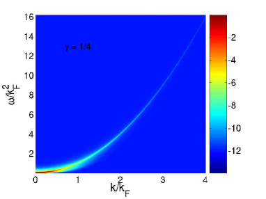
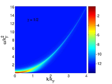
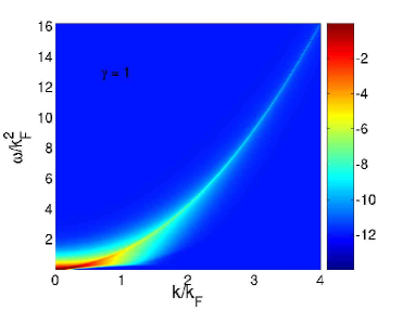
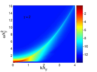
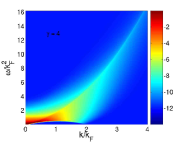
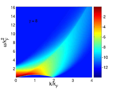
Figure 1: Pseudocolor plots of the logarithm of the dynamical one-body correlation function of the Lieb-Liniger gas, for $\gamma=1/4,1/2,1,2,4$ and $8$. The data was obtained from systems at unit density and $N=150$ particles. The horizontal axis is momentum, and the vertical one energy. Sum rule saturations are listed in Table 1. At small $\gamma$, the correlation weight at fixed momentum falls mostly around the Type I dispersion relation.

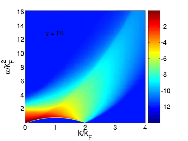
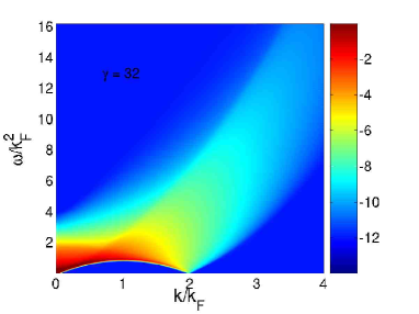
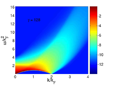
Figure 2: Same as Figure 1, but now for $\gamma=16,32,64$ and $128$, showing the progression of the distribution of correlation weight in the strongly-interacting regime. As $\gamma$ increases, more correlation weight gets concentrated near the lower threshold.

4.1 Results

Table 1: Sum rule saturation percentages achieved as a function of the interaction parameter, for various values of $N$. The last line gives the contribution coming from states outside of the sub-Fock space used for the numerics, as computed from the asymptotic form of the static correlator (see text).

$N,\gamma$	1/4	1/2	1	2	4	8	16	32	64	128
$50$	100	100	100	99.99	99.98	99.96	99.94	99.92	99.91	99.91
$100$	100	100	99.99	99.98	99.96	99.92	99.85	99.81	99.78	99.75
$150$	100	99.99	99.98	99.95	99.91	99.71	99.61	99.33	99.44	99.20
$200$	99.99	99.96	99.92	99.87	99.64	99.28	98.83	98.59	98.43	98.33
$k>4k_{F}$	$2\cdot 10^{-4}$	$8\cdot 10^{-4}$	0.003	0.007	0.018	0.032	0.047	0.058	0.064	0.067

Our results for the dynamical one-body correlation function (5) for different values of $\gamma$ are presented in Figures 1 and 2 as density plots. To obtain continuous curves, the energy delta functions in (48) are smoothened into Gaussians of width slightly larger than the typical interlevel spacing. The color coding of these figures follows the logarithm of the correlation function. All data presented in these was obtained by considering systems of $N=150$ particles with unit density. For each individual plot, around seventy million intermediate states were taken into account, yielding extremely good saturation of the sum rule (49), as summarized in Table 1. The summation we actually perform is restricted to intermediate states within a window of momentum $k\in[0,4k_{F}]$, composed of (possibly many) single-particle excitations of momentum $|k|<k_{max}=8k_{F}$. The correlation weight carried by states outside of this sub-Fock space is negligible, as can be clearly seen from the sum rule saturations achieved. This can also be independently checked because the large $k$ tail of the static correlation function is exactly known from [42] (as discussed more extensively in the next section, see Eq. (55) below). In the last row of Table 1 we report the contributions calculated from Eq. (55) for all the states with $k>4k_{F}$. We checked that the error due to finite $N$ and to subleading corrections to Eq. (55) do not change the accuracy we reported. From these data it is evident that states with $k>4k_{F}$ contribute for almost all the missing part for $N=50$ and for a relevant part for $N=100$. In all cases, the (rest of the) missing part of the sum rules is therefore ascribed to intermediate states within the sub-Fock space we consider, but which we do not include in the summation. In fact, our sum only considers an extremely small fraction of all the available intermediate states within the sub-Fock space, made of only a handful of elementary excitations. The distribution of correlation weight between $0,2,4,6$ and $8$ particle states for a given value $\gamma=16$ for different values of $N$ is given in Table 2 (here, $2n$ particle states are made from $n$ particle-hole excitations on the ground state of $N-1$ particles). These numbers represent lower bounds of the contributions from the different classes of states. There are large variations of this distribution as a function of $N$, although the full correlator itself remains more or less invariant. The general scenario is that $0$ and $2$ particle contributions are strictly decreasing functions of $N$, while higher particle number contributions first increase and thereafter decrease, with a maximum at $N^{max}_{2n}$ such that $N^{max}_{2n}>N^{max}_{2m}$ if $n>m$. As a function of $\gamma$, we observe as naturally expected that for small $\gamma$, intermediate states with smaller (larger) numbers of particles carry more (less) weight, with more weight shifting to higher particle numbers when $\gamma$ increases.

We also provide in the left panels of Figures 3 and 4 a series of fixed-momentum cuts for a number of values of the interaction parameter, with data for two different system sizes, smoothened as explained above (without smoothing, these would be $\delta$ peaks; the smoothing however blurs the lower threshold slightly). At small $\gamma$, the correlation is peaked around the Type I dispersion relation. As the interaction parameter increases, the peak becomes broader and moves towards lower energies, as expected in view of the increasing fermion-like nature of the system. At intermediate values of $k$, the correlation width also increases with $\gamma$, with the peaks eventually shifting altogether from high to low energies. The difference between the $N=100$ and $N=150$ curves can mostly be ascribed to imperfect sumrule saturation (the logarithm of the correlation function is plotted, and therefore the actual difference between curves lies in regions where the correlation weight is extremely small).

On the right panels of these figures, the same data sets are used to plot the integrated correlation,

$$G^{I}_{2}(k,\omega)=\int_{0}^{\omega}d\omega^{\prime}G_{2}(k,\omega)=$$

$$=2\pi L\sum_{\{\mu\}_{N-1}}\Theta(\omega^{\prime}-E_{\{\mu\}}+E_{\{\lambda\}})\delta_{k,P_{\{\mu\}}-P_{\{\lambda\}}}G(\{\mu\},\{\lambda\}),$$ (50)

for which no smoothing procedure is necessary. These curves are in fact series of steps of height corresponding to the correlation weight of any intermediate state lying at this point in $k$, $\omega$ space. In the infinite size limit, these would become smooth curves whose $\omega$ derivative would be the one-body correlation function. The discreteness of the steps due to the finite number of particles can just be made out in the plots. The fact that no artificial smoothing of the delta functions is used in these data sets makes them the most appropriate objects for eventual comparison with other theoretical or numerical methods (as e.g. those employed in Refs. [43] for the dynamical structure factor).

Table 2: Distribution of sum rule weight between intermediate states involving $N_{p}$ particles, with $N_{p}=0,2,4,6$ and $8$. The numbers given are the fraction of the total sumrule associated to each sub-type of excited state which was obtained during the runs. We present data for $\gamma=16$, for three values of $N$. These are lower bounds only, since we only scan over a very small fraction of the total number of multiparticle states.

$N,N_{p}$	0	2	4	6	8	TT
50	0.29075	0.47437	0.22541	0.00877	0.00006	0.99936
100	0.22157	0.46575	0.29119	0.01979	0.00018	0.99848
150	0.18881	0.45288	0.32627	0.02813	—	0.99609

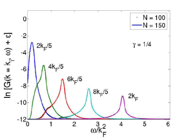
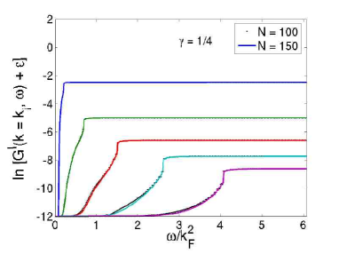
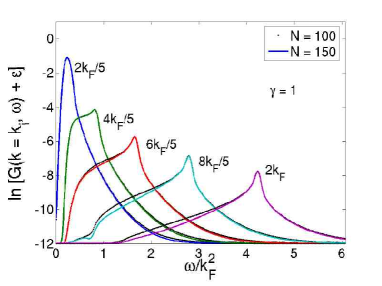
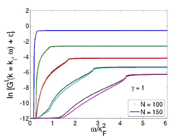
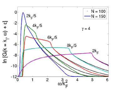
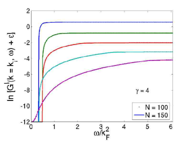
Figure 3: Left: fixed-momentum cuts of the logarithm of the one-body correlation function, for $\gamma=1/4,1$ and $4$. As $\gamma$ increases, the peaks widen. Right: logarithm of the integrated correlation function (50) for the same values of $k$ and $\gamma$ ($\varepsilon=10^{-12}$ is a regulator for the logarithm).

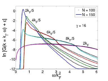
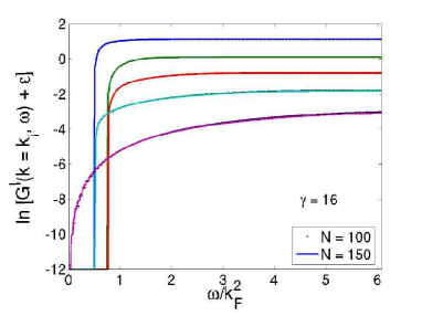
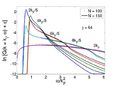
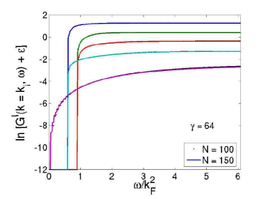
Figure 4: Same as above, now for $\gamma=16$ and $64$. The peaks have moved to low energy.

5 Momentum distribution function and one-body density matrix

From the data of the dynamical one-particle correlation function presented in the previous section it is very easy to recover the static correlation function

$$n(k)=\int_{0}^{\infty}\frac{d\omega}{2\pi}G_{2}(k,\omega)\,.$$ (51)

$n(k)$ represents the relative occupation of the single particle state of momentum $k$ and is consequently known as the momentum distribution function. It is the quantity that is directly measured in the ballistic expansion of a trapped gas (see e.g., the review [44]). Its Fourier transform is the one-body density matrix

$$\rho(x) = \sum_{s=-\infty}^{\infty}n\left(\frac{2\pi s}{L}\right)\cos\left(\frac{2\pi xs}{L}\right)$$ (52)

$$= \frac{\int_{0}^{L}\Psi^{*}_{0}(x_{1}+x,x_{2},\dots,x_{N})\Psi_{0}(x_{1},x_{2},\dots,x_{N})dx_{2}\dots dx_{N}}{\int_{0}^{L}|\Psi_{0}(x_{1},x_{2},\dots,x_{N})|^{2}dx_{1}\dots dx_{N}}\,,$$ (53)

where $\Psi_{0}(x_{1},x_{2},\dots,x_{N})$ is the $N$-body ground-state wavefunction. $\rho(x)$ is the reduced density matrix of a single particle when all the other degrees of freedom have been integrated out.

Given its theoretical and experimental importance, the momentum distribution function is the correlation function that has been mostly studied in the literature. In the TG limit, its exact expression is known since the work of Lenard [19]: for finite $N$ and $L$, $\rho(x)$ can be written as a simple Toeplitz determinant (see also [45]) and the momentum distribution function can be readily obtained via Fourier transform. The Lenard formula has been re-obtained in the framework of algebraic Bethe Ansatz in Ref. [22]. Some analytical asymptotic expansions in the TG limit have been reported in Refs. [46, 21, 45, 47] and a $1/\gamma$ expansion has been developed in [48]. We mention that these results have been recently generalized to a lattice of impenetrable bosons [49] and to anyonic gases [50].

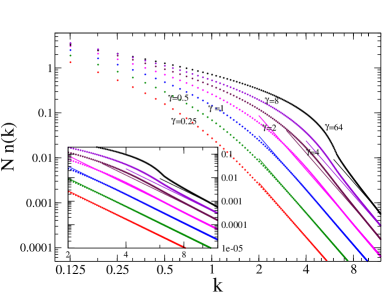
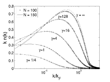
Figure 5: Momentum distribution function for some representative value of $\gamma$. Left: $n(k)$ in log-log scale. In the inset the large momentum section of and the asymptotic $k^{-4}$ law. Right: plot of $kn(k)$ as function of $k$ in log-scale (this can be conveniently compared with the data of Ref. [55]). The exactly known Tonks-Girardeau ($\gamma\rightarrow\infty$) limit is plotted as reference.

In the case of finite coupling constant, only the asymptotic expansion for small and large momenta are known. The infrared behavior can be obtained from the hydrodynamic theory of low-energy excitations [51]

$$n(k)\propto k^{\alpha-1}\,,$$ (54)

where $\alpha=v_{s}/(4\pi n)$ and $v_{s}$ is the speed of sound. The above result holds for $k\ll\xi^{-1}$, where $\xi=\sqrt{2}/v_{s}$ is the healing length. The corresponding behavior of the one-body density matrix is $\rho(x)\propto x^{-\alpha}$ for $x\gg\xi$. The exponent $\alpha$ interpolates between $0$ and $1/2$ when the coupling constant $\gamma$ is increased from $0$ to $\infty$. The large momentum tail can be elegantly obtained by using simple theorems on the Fourier transform [42] and can be related to the previously calculated second moment of the density operator [24], yielding ($n(k)$ corresponds to $w(p)$ in Ref. [42] and not to $W(p)$)

$$Nn(k)={\gamma^{2}e^{\prime}(\gamma)}\left(\frac{n}{k}\right)^{4}\,,\qquad{\rm for}\,\;k\to\infty$$ (55)

where $e(\gamma)$ is the ground-state energy per particle in the thermodynamic limit (in the TG limit this formula was previously obtained in Ref. [47, 45]). Similarly a small $x$ expansion can be written for the one-body density matrix:

$$\frac{\rho(x)}{n}=1+\sum_{i=1}^{\infty}c_{i}|nx|^{i}\,.$$ (56)

The $k^{-4}$ law for $n(k)$ implies that the lowest odd power in this Taylor expansion is $|x|^{3}$, thus $c_{1}=0$. The coefficient $c_{3}$ is easily read from Eq. (55), yielding $c_{3}=\gamma^{2}e^{\prime}(\gamma)/12$ [42]. $c_{2}$ can be obtained [42] using the Hellmann-Feynman theorem: $c_{2}=-1/2[e(\gamma)-\gamma e^{\prime}(\gamma)]$. The other coefficients $c_{i}$ with $i>3$ are still unknown.

To the best of our knowledge the results reported above are all that is exactly known about the momentum distribution function (some results for finite and small $N$ are reported in Ref. [52]). In particular nothing is known for finite coupling in the intermediate window of momenta, that is actually the region easier to access in experiments (in fact the infrared behavior is usually obscured by the harmonic trap, see e.g. [7, 53, 54, 55, 56]). As a consequence, up to now this interesting regime has been investigated only with purely numerical methods as Quantum Monte Carlo [55] and density matrix renormalization group [53]. However, these methods, although very powerful, were unable to describe all the physics from the infrared to the ultraviolet. Our results demonstrate that the ABACUS method is able to do this.

In Fig. 5 we present $n(k)$ as function of $k$ for several values of the interacting parameter and for $N=100,150$. The curves clearly show that finite size effects are negligible on this scale. We also plot $kn(k)$ for comparison with the Quantum Monte Carlo data of Ref. [55]: the data shows an overall qualitative agreement. The exact result of Lenard for the TG limit is also given for comparison.

One advantage of our method is that we are able to reproduce the $k^{-4}$ law to high accuracy. In the inset of Fig. 5 we plot $n(k)$ versus $k$ for large momenta and for several values of $\gamma$. The $k^{-4}$ tails are evident, and agree with the asymptotic curves predicted from Eq. (55). We stress that in these curves there is no fitting parameter, both the power-law and the numerical prefactor are fixed according to Eq. (55). This therefore confirms that our method provides accurate results even at high momentum.

Now we turn to the real spatial dependence of this correlation function. From our data, the one-body density matrix is easily obtained by means of Fourier transform according to Eq. (53). In Fig. 6 we plot $\rho(x)$ as function of $x/L$ for some values of $\gamma$. The inset in log-log scale clearly shows the power-law behavior $x^{-\alpha}$ for $x\gg\xi$ (but smaller than $L/2$). At large distances there are evident deviations due to the finiteness of the system. Conformal field theory [57] predicts that for periodic boundary conditions the correlation function gets modified according to

$$\rho(x)\propto\left(\frac{\pi}{L\sin(\pi x/L)}\right)^{\alpha}\,.$$ (57)

For $x\ll L$, this form reproduces the power-law $x^{-\alpha}$, but it also completely describes the behavior for any $x$ with the only condition $x\gg\xi$. In fact, plotting $L^{\alpha}\rho(x)$ versus $x/L$ all the curves for various values of $N$ fall on the same master curve, which depends on $\gamma$ only through the exponent $\alpha$. The proportionality constant in Eq. (57) can be fixed by imposing a given value at $x=L/2$, but in Fig. 6 we let it free and consequently there is no fitting parameter again. It is evident that only for very small value of $x/L$ it is possible to notice the effect of the finite healing length $\xi$.

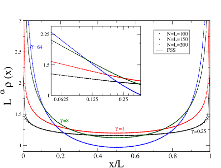
Figure 6: One-body density matrix $\rho(x)$ for $\gamma=64,8,1,0.25$ and $N=100,150,200$ compared with the finite-size scaling (FSS) form. Inset: The same plot in log-log scale to show the power law behavior for $\xi\ll x<L/2$.

The small $x$ behavior is also easily accessed with ABACUS. In Fig. 7 we report $\rho(x)$ for very small $x$ (up to $x=1$) for $N=100$. Compared to Fig. 6 we are now showing a very small fraction of the total plot. The numerical data are compared with the Taylor expansion Eq. (56) with the coefficients $c_{2}$ and $c_{3}$ evaluated in Ref. [42]. For very small $x$ the agreement is perfect and again there is no fitting parameter. However, we notice that Eq. (56) with only two $c_{i}$’s describes a very limited region, probably very difficult to reach in real systems. A curious fact can be easily deduced from Fig. 6: the correction to the asymptotic result is positive for large $\gamma$ and negative for small values, so the unknown coefficient $c_{4}$ changes sign as $\gamma$ increases (contrary to $c_{2}$ and $c_{3}$, which are always respectively negative and positive). From our data, this change should occur around $\gamma\sim 8$.

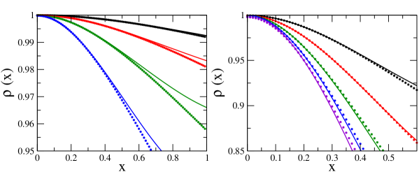
Figure 7: Small $x$ behavior of the one-body density matrix $\rho(x)$, compared with the asymptotic result Eq. (56). Left: $\gamma=0.25,0.5,1,2$ from top to bottom. Right: $\gamma=4,8,16,32,64$ from top to bottom.

6 Conclusion

In conclusion, we have presented results for the one-body dynamical correlation function of the one-dimensional Bose gas (Lieb-Liniger model) by using the ABACUS method, mixing integrability and numerics. We obtained the full momentum and frequency dependence of the correlations, for values of the interaction parameter interpolating continuously from the weakly-interacting regime to the strongly-interacting Tonks-Girardeau regime. We wish to stress that the present method not only yields previously inaccessible results on the dynamics, but by extension also allows to go beyond other methods when restricting to static quantities. For example, we have showed how our results, integrated to recover the static correlation function, are the first to be in agreement with all asymptotic predictions.

We hope that our results will provide motivation for further experimental work on quasi-one-dimensional gases, in particular on the direct observation of dynamical correlation functions in these systems. On the other hand, we intend to use the correlation functions we have obtained for the idealized Bose gas as a starting point for addressing more general situations, including the effects of intertube coupling and/or confining potential. Other possibilities include the study of entanglement in this stongly-correlated system, using measures expressible in terms of simple combinations of the correlation functions we have studied. We will report on these issues in future publications.

References

References

- [1] H. A. Bethe, Zeitschrift für Physik 71, 205 (1931).
-
[2]
E. H. Lieb and W. Liniger, Phys. Rev. 130, 1605 (1963);
E. H. Lieb, Phys. Rev. 130, 1616 (1963). - [3] A. Görlitz, J. M. Vogels, A. E. Leanhardt, C. Raman, T. L. Gustavson, J. R. Abo-Shaeer, A. P. Chikkatur, S. Gupta, S. Inouye, T. P. Rosenband, D. E. Pritchard, W. Ketterle, Phys. Rev. Lett. 87, 130402 (2001).
- [4] M. Greiner, I. Bloch, O. Mandel, T. W. Hänsch and T. Esslinger, Phys. Rev. Lett. 87, 160405 (2001).
- [5] M. Greiner, O. Mandel, T. Esslinger, T. W. Hänsch and I. Bloch, Nature 415, 39 (2002).
- [6] H. Moritz, T. Stöferle, M. Köhl and T. Esslinger, Phys. Rev. Lett. 91, 250402 (2003).
- [7] B. Paredes, A. Widera, V. Murg, O. Mandel, S. Falling, I. Cirac, G. V. Shlyapnikov, T. W. Hänsch and I. Bloch, Nature 429, 277 (2004).
- [8] T. Kinoshita, T. Wenger and D. S. Weiss, Science 305, 1125 (2004).
- [9] M. Köhl, T. Stöferle, H. Moritz, C. Schori and T. Esslinger, Appl. Phys. B 70, 1009 (2004).
- [10] C. D. Fertig, K. M. O’Hara, J. H. Huckans, S. L. Rolston, W. D. Phillips and J. V. Porto, Phys. Rev. Lett. 94, 120403 (2005).
- [11] T. Kinoshita, T. Wenger and D. S. Weiss, Nature 440, 900 (2006).
- [12] L. Tonks, Phys. Rev. 50, 955 (1936).
-
[13]
M. Girardeau, J. Math. Phys. (N.Y.) 1, 516 (1960);
M. Girardeau, Phys. Rev. 139, B500 (1965). - [14] M. Gaudin, “La fonction d’onde de Bethe”, Masson (Paris) (1983).
- [15] V. E. Korepin, N. M. Bogoliubov and A. G. Izergin, “Quantum Inverse Scattering Method and Correlation Functions”, Cambridge, 1993, and references therein.
- [16] M. Takahashi, “Thermodynamics of One-Dimensional Solvable Models”, Cambridge, 1999, and references therein.
- [17] D. C. Mattis, “The Many-body Problem”, World Scientific, Singapore, 1993.
- [18] C. N. Yang and C. P. Yang, J. Math. Phys. (N.Y.) 10, 1115 (1969).
- [19] A. Lenard, J. Math. Phys. 5, 930 (1964).
- [20] A. Lenard, J. Math. Phys. 7, 1268 (1966).
- [21] M. Jimbo, T. Miwa, Y. Mori and M. Sato, Physica 1D, 80 (1980).
- [22] V. E. Korepin and N. A. Slavnov, Commun. Math. Phys. 129, 103 (1990).
- [23] K. V. Kheruntsyan, D. M. Gangardt, P. D. Drummond and G. V. Shlyapnikov, Phys. Rev. Lett. 91, 040403 (2003).
- [24] D. M. Gangardt and G. V. Shlyapnikov, Phys. Rev. Lett. 90, 010401 (2003).
- [25] D. M. Gangardt and G. V. Shlyapnikov, New Jour. Phys. 5, 79.1 (2003).
-
[26]
M. A. Cazalilla, Phys. Rev. A 67, 53606 (2003);
M.T. Batchelor and X.-W. Guan, Laser Phys. Lett. 4, 77 (2007) [cond-mat/0608624]. -
[27]
V. V. Cheianov, H. Smith and M. B. Zvonarev,
Phys. Rev A 73, 51604 (2006) [cond-mat/0506609];
V. V. Cheianov, H. Smith and M. B. Zvonarev, J. Stat. Mech. (2006) P08015 [cond-mat/0602468]. - [28] A. A. Belavin, A. M. Polyakov and A. B. Zamolodchikov, Nucl. Phys. B 241, 333 (1984).
- [29] P. Di Francesco, P. Mathieu and D. Sénéchal, Conformal Field Theory, Springer, 1997.
- [30] V. E. Korepin and N. A. Slavnov, Commun. Math. Phys. 136, 633 (1991).
- [31] T. Kojima, V. E. Korepin and N. A. Slavnov, Commun. Math. Phys. 188, 657 (1997).
- [32] T. Kojima, V. E. Korepin and N. A. Slavnov, Commun. Math. Phys. 189, 709 (1997).
- [33] A. R. Its and N. A. Slavnov, Teor. Mat. Fiz. 119, 179 (1999).
- [34] N. A. Slavnov, Teor. Mat. Fiz. 121, 117 (1999).
- [35] J.-S. Caux and J. M. Maillet, Phys. Rev. Lett. 95, 077201 (2005).
- [36] J.-S. Caux, R. Hagemans and J. M. Maillet, J. Stat. Mech. (2005) P09003.
- [37] J.-S. Caux and P. Calabrese, Phys. Rev. A 74, 031605(R) (2006).
- [38] N. A. Slavnov, Teor. Mat. Fiz. 79, 232 (1989); ibid., 82, 389 (1990).
- [39] Algebraic Bethe Ansatz Computation of Universal Structure factors. See http://staff.science.uva.nl/jcaux/ABACUS.html.
- [40] L. D. Faddeev, E. K. Sklyanin and L. A. Takhtajan, Theor. Math. Phys. 40, 688 (1980).
- [41] V. E. Korepin, Commun. Math. Phys. 86, 391 (1982).
- [42] M. Olshanii and V. Dunjko, Phys. Rev. Lett. 91, 090401 (2003).
-
[43]
J. Brand and A. Yu. Cherny, Phys. Rev. A 72, 033619 (2005);
A. Yu. Cherny and J. Brand, Phys. Rev. A 73, 023612 (2006);
G. G. Batrouni et al, Phys. Rev. A 72, 031602 (2005);
M. Gattobigio, J. Phys. B 39, S191 (2006). - [44] W. Ketterle, D.S. Durfee, D.M. Stamper-Kurn, Contribution to the proceedings of the 1998 Enrico Fermi summer school on Bose-Einstein condensation in Varenna, Italy [cond-mat/9904034].
- [45] P. J. Forrester, N. E. Frankel, T. M. Garoni and N. S. Witte, Phys. Rev. A 67, 43607 (2003) [cond-mat/0211126]
-
[46]
H. G. Vaidya and C. A. Tracy, Phys. Rev. Lett. 42, 3(1979);
H. G. Vaidya and C. A. Tracy, Phys. Rev. Lett. 43, 1540 (1979). - [47] A. Minguzzi, P. Vignolo and M. P. Tosi, Phys. Lett. A 294, 222 (2002).
-
[48]
D. B. Creamer, H. B. Thacker and D. Wilkinson,
Phys. Rev. D 23, 3081 (1981);
M. Jimbo and T. Miwa, Phys. Rev. D 24, 3169 (1981). -
[49]
D. M. Gangardt, J. Phys. A 37, 9335 (2004);
D. M. Gangardt and G. V. Shlyapnikov, New J. of Phys. 8, 167 (2006). - [50] R. Santachiara, F. Stauffer and D. C. Cabra, cond-mat/0610402.
-
[51]
L. Reatto and G. V. Chester, Phys. Rev. 155, 88 (1967);
M. Schwartz, Phys. Rev. B. 15, 1399 (1977);
F. D. M. Haldane, Phys. Rev. Lett. 47, 1840 (1981). - [52] P. J. Forrester, N. E. Frankel and M. I. Makin, Phys. Rev. A 74, 43614 (2006).
- [53] B. Schmidt and M. Fleischhauer, cond-mat/0608351.
- [54] T. Paperbrock, Phys. Rev. A 67, 41601 (2003).
- [55] G. E. Astrakharchik and S. Giorgini, Phys. Rev. A 68 , 31602 (2003).
- [56] D. L. Luxat and A. Griffin, Phys. Rev. A 67, 043603 (2003).
- [57] See, e.g., chapter 11 in J. Cardy, Scaling and renormalization in Statistical Physics, Cambridge University Press.