Symmetric and asymmetric states in a mesoscopic superconducting wire in the voltage driven regime

Abstract

The response of a mesoscopic homogeneous superconducting wire, connected with bulk normal metal reservoirs, is investigated theoretically as function of the applied voltage. The finite relaxation length of the nonequilibrium quasiparticle distribution function $\overline{L_{E}}$ is included where we assumed that our wire is in the dirty limit. We found that both symmetric and asymmetric states can exist which are characterized by a stationary symmetric and asymmetric distribution of the order parameter with respect to the center of the wire. Current voltage characteristics of the wire with length $L>\overline{L_{E}}$ being in the symmetric state show a pronounced S-behavior. The asymmetric state may exist only for voltages larger than some critical value and coexist with the symmetric state in a finite voltage interval. For wires with $L\sim\overline{L_{E}}$ the asymmetric state survives up to higher values of the voltage than the symmetric one and may exist both in the voltage and the current driven regimes. We propose an experiment to observe reversible switching between those stationary symmetric and asymmetric states.

I Introduction

Modifications of the quasiparticle distribution function $f(E)$ in a superconductor will drastically influence its properties. Injection(extraction) of the quasiparticles via a tunnel junction suppresses(enhances) the superconducting gap Chi ; Blamire and creates a charge imbalance in the sample Clarke ; external electro-magnetic radiation excites quasiparticles to higher energy levels and can considerably increase the superconducting gap and the critical current Dmitriev ; Eliashberg ; moving vortices will change $f(E)$ resulting in the dependence of the vortex viscosity on the vortex velocity Larkin ; fast oscillations of the superconducting gap in superconducting bridges or in phase slip centers leads to a dynamical nonequilibrium distribution $f(E)$ and results in strongly nonlinear current-voltage characteristics Tinkham .

Recently, the effect of nonequilibrium $f(E)$ induced by an applied voltage was studied in a dirty superconducting wire (whose mean path length $\ell$ is smaller than the coherence length at zero temperature $\xi_{0}$) that was connected to large normal metal reservoirs with no tunnel barriers Keizer . Theoretically it was found that there is a critical voltage $V_{c}$ above which the superconductor exhibits a first order transition to the normal state. This effect is connected with a strong modification of the quasiparticle distribution function $f(E)$ and especially its odd part $f_{L}(E)=f(-E)-f(E)$, by the applied voltage. The applied voltage leads to the excitation of quasiparticles to energy levels near the energy gap resulting in a strong modification (i.e. diminishing) of the order parameter.

In the present work we study the same system as Ref. Keizer but include the finite relaxation time $\tau_{E}$ of the nonequilibrium quasiparticle distribution function $f(E)$ due to inelastic electron-phonon interaction which was neglected in Ref. Keizer . We show, that the finite length $\overline{L_{E}}=\sqrt{\tau_{E}D}$ ($D$ is the diffusion constant) weakens the effect of the applied voltage on the superconducting properties and changes qualitatively the shape of the IV characteristic (it becomes S-shaped) already for wires with length $L$ of several $\overline{L_{E}}$. Furthermore we find that in our homogeneous wire there are stationary states with both symmetric and asymmetric distributions of the order parameter (with respect to the center of the wire). The asymmetric state exists only at voltage larger than some critical value and can coexist with the stationary symmetric states in a finite voltage interval. For wires with length $L\sim\overline{L_{E}}$ it survives up to larger applied voltages than the symmetric one and at specific conditions even for larger currents.

The paper is organized as follows. In section II we present our theoretical model. In sections III and IV we discuss the existence of the symmetric and asymmetric states, respectively. Finally, in section V we present our conclusions and propose an experimental setup to observe the reversible transitions between the predicted symmetric and asymmetric states.

II Model

We used a quasi-classical approach to calculate the nonequilibrium properties of a superconductor in the dirty limit and restrict ourselves to temperatures near $T_{c}$. This allows us to use the Usadel equation Usadel for the normal $\alpha(E)=\cos\Theta$ and anomalous $\beta(E)=\sin\Theta$ quasi-classical Green functions in relatively simple form Schmid ; Kramer ; Watts-Tobin

$$\frac{d^{2}\Theta}{dx^{2}}+((2iE-\frac{1}{L_{E}^{2}})-(\nabla\varphi)^{2}\cos\Theta)\sin\Theta+2|\Delta|\cos\Theta=0.$$ (1)

In the same limit the diffusive type equation for the space dependence of the transverse (even in energy) $f_{T}(E)=1-f(E)-f(-E)$ and longitudinal (odd in energy) $f_{L}(E)=f(-E)-f(E)$ parts of the quasiparticle distribution function $2f(E)=1-f_{L}(E)-f_{T}(E)$ are given by

$$\nabla((N_{1}^{2}-R_{2}^{2})\nabla f_{L})+2N_{2}R_{2}\nabla\varphi\nabla f_{T}$$

$$-\frac{N_{1}}{L_{E}^{2}}(f_{L}-f_{L}^{0})=0,$$ (2a)

$$\nabla((N_{1}^{2}+N_{2}^{2})\nabla f_{T})+2N_{2}R_{2}\nabla\varphi\nabla f_{L}-$$

$$\frac{N_{1}}{L_{E}^{2}}(f_{T}-\phi\frac{\partial f_{L}^{0}}{\partial E})-2N_{2}|\Delta|f_{T}=0.$$ (2b)

Here $\varphi$ is the phase of the order parameter $\Delta=|\Delta|e^{i\phi}$, $\phi$ is an electrostatic potential, $N_{1}(E)+iR_{1}(E)=\cos\Theta(E)$, $N_{2}(E)+iR_{2}(E)=\sin\Theta(E)$ and $f_{L}^{0}(E)=\tanh(E/2T)$ is the odd part of the equilibrium Fermi-Dirac distribution function of the quasiparticles. The dimensionless length $L_{E}=\sqrt{D\tau_{E}}/\xi_{0}=\sqrt{\tau_{E}\Delta_{0}/\hbar}$ defines the range over which the nonequilibrium distribution of the quasiparticles may exist in the sample.

Within the same approach we have the rather simple self-consistent stationary equation for the order parameter $\Delta$

$$a_{1}\frac{d^{2}\Delta}{dx^{2}}+(1-a_{2}|\Delta|^{2}+\Psi_{1}+i\Psi_{2})\Delta=0,$$ (3)

which is analogous to the Ginzburg-Landau equation Thinkham but with the additional terms $\Psi_{1}=\int_{0}^{\infty}R_{2}(f_{L}-f_{L}^{0})dE/|\Delta|$ and $\Psi_{2}=\int_{0}^{\infty}N_{2}f_{T}dE/|\Delta|$. Because we are interested in a stationary solution we removed all time-dependent terms in Eq. (2-3) which are present in the original equations. Schmid ; Kramer ; Watts-Tobin

In Eqs. (1-3) the order parameter $\Delta$ is scaled by the zero-temperature value of the order parameter $\Delta_{0}\simeq 1.76k_{B}T_{c}$ (in weak coupling limit), distance is in units of the zero temperature coherence length $\xi_{0}=\sqrt{\hbar D/\Delta_{0}}$ and temperature in units of the critical temperature $T_{c}$. Because of this choice of scaling the numerical coefficients in Eq. (3) are $a_{1}\simeq 0.69$ and $a_{2}\simeq 0.33$. The current is scaled in units of $j_{0}=\Delta_{0}/(\xi_{0}\rho_{n}e)$ and the electrostatic potential is in units of $\phi_{0}=\Delta_{0}/e$ ($\rho_{n}$ is the normal state resistivity and $e$ is the electric charge).

The deviation of $f_{L}(E)$ from its equilibrium value $f_{L}^{0}$ may considerably influence the value of the order parameter through the term $\Psi_{1}$. The nonzero $f_{T}(E)$ is mainly responsible for the appearance of the charge imbalance in the superconductor and the conversion of the normal current to the superconducting one and vice versus. The latter one occurs due to the Andreev reflection process (term $2N_{2}|\Delta|f_{T}$ in Eq. (2b)) or/and due to inelastic electron-phonon interaction (term $N_{1}(f_{T}-\phi\partial f^{0}/\partial E)/L_{E}^{2}$ in Eq. (2b)).

The system of Eqs. (1-3) was numerically solved using an iterative procedure. First Eq. (3) was solved by the Euler method (we add a term $\partial\Delta/\partial t$ in the right hand side of Eq. (3)) until $|\Delta|$ became time independent. Than Eqs. (1-2) were solved from which we obtained new potentials $\Psi_{1}$ and $\Psi_{2}$ which were then inserted in Eq. (3). This iterations process was continued until convergence was reached. In some voltage interval no convergence was reached and we identify it as the absence of stationary solutions to Eqs. (1-3). Thus our numerical procedure automatically checks the stability of the found stationary symmetric and asymmetric states.

The numerical solution of Eqs. (1-3) converges much faster than the equivalent but more complicated Eqs. (5,7,8,9) in Ref. Keizer . This allowed us to consider on the one hand a rather large interval of parameters but on the other hand it restricts the validity of the obtained results to the temperature interval $0.9<T/T_{c}<1$ which roughly corresponds to the validity condition $\Delta(T)/k_{B}T_{c}\ll 1$ of Eqs. (1-3)Watts-Tobin .

Knowing the solution of Eqs. (1-3) the current in the system can be found using the following equation

$$j=2a_{1}|\Delta|^{2}\nabla\varphi$$

$$+\int_{0}^{\infty}\left((N_{1}^{2}+N_{2}^{2})\nabla f_{T}+2N_{2}R_{2}f_{L}\nabla\varphi\right)dE.$$ (4)

The first term in Eq. (4) may be identified as a superconducting current and the second one as a normal one. Assuming that the effect of the free charges is negligible in the superconductors the electrostatic potential is determined by the following expression

$$\phi=\int_{0}^{\infty}N_{1}f_{T}dE.$$ (5)

We used the following boundary conditions for the system of Eqs. (1-3)

$$\Theta(\pm L/2)=\Delta(\pm L/2)=0,$$ (6a)

$$f_{L}(\pm L/2)=\frac{1}{2}\left(\tanh\left(\frac{E+V(\pm L/2)}{2T}\right)+\tanh\left(\frac{E-V(\pm L/2)}{2T}\right)\right),$$ (6b)

$$f_{T}(\pm L/2)=\frac{1}{2}\left(\tanh\left(\frac{E+V(\pm L/2)}{2T}\right)-\tanh\left(\frac{E-V(\pm L/2)}{2T}\right)\right),$$ (6c)

which models the situation where there is a direct electrical contact of our superconducting wire of length L with large normal metal reservoirs at an applied voltage $V(\pm L/2)$.

III Symmetric states

In Fig. 1 we present our calculated current-voltage (IV) characteristics of the superconducting wire with length $L=100$, temperature $T=0.98$ and different $L_{E}$. In this section we consider the case of symmetric applied voltage $V(\pm L/2)=\mp V$.

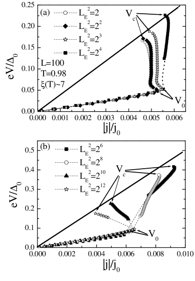
Figure 1: Current-voltage characteristics of the superconducting wire with length $L=100$, temperature $T=0.98$ and different relaxation lengths $L_{E}$. Figure (a) corresponds to the case $L_{E}<\xi(T)\sim 7$ and figure (b) to the case $L_{E}\gg\xi(T)$. Solid line shows the IV characteristic in the normal state. Dashed lines in both (a) and (b) mark the voltage interval where there are no stationary solutions to Eqs. (1-3).

When $L_{E}\lesssim\xi(T)\ll L$ the $f_{L}(E)$ decays on the scale of the coherence length and practically does not influence the value of the order parameter. When the current density in the wire exceeds the critical value (marked by $V_{0}$ in Fig. 1), the N-S borders (formed near the ends of the wire due to the boundary condition Eq. (6c)) become unstable and start to move to the center of the wire. The superconducting region decreases and it effectively increases the resistance of the whole sample leading to a decrease of the current up to its critical value. This process results in the ”vertical line”-like region in the IV characteristics of the wire. The longer the sample, the wider will be this ”vertical line”-like region. Finally, at the critical voltage $V_{c}$ the region where $|\Delta|\neq 0$ is reduced to about $\xi(T)$ and a first order phase transition to the normal state occurs.

In this limit we may use the so called ’local equilibrium model’ which leads to the extended time-dependent Ginzburg-Landau (TDGL) equations Kramer ; Watts-Tobin . A simple analysis based on those equations Vodolazov shows an increasing critical current with a stable N-S border when increasing the parameter $\gamma=2\tau_{E}\Delta_{0}/\hbar=2L_{E}^{2}$. This is the reason for the increase of the maximal possible current in Fig. 1(a) for small values of $L_{E}$. A direct comparison with results calculated within the extended TDGL equations (see Fig. 2) show qualitatively the same behavior.

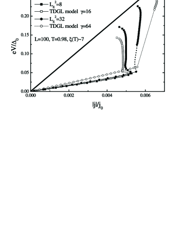
Figure 2: Comparison of the results obtained through solution of Eqs. (1-3) with results of a numerical solution of the extended TDGL equations. Up to $L_{E}\sim\xi(T)$ the extended TDGL equations gives qualitatively the same results. Dashed lines mark the voltage interval where no stationary solutions of Eqs. (1-3) and the TDGL equations can be found.

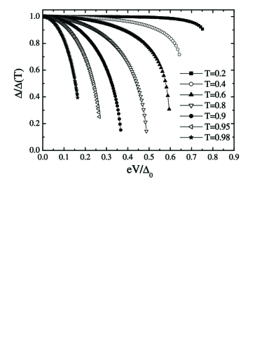
Figure 3: Dependence of the order parameter on the parameter V as obtained from Eq. (7) for different temperatures.

In the opposite limit $L_{E}\sim L\gg\xi(T)$ the nonzero $f_{L}(E)$ considerably affects the value of the order parameter everywhere in the sample. In Ref. Keizer it was shown for $T=0$ and $L_{E}=\infty$, that when the applied voltage is of about $\Delta_{0}$ the superconducting order parameter vanishes everywhere in the sample and it leads to a first order phase transition to the normal state. Actually, qualitatively the same is true for arbitrary temperature: when the voltage reaches approximately $\Delta(T)$ the order parameter starts to decrease rapidly. In Fig. 3 we show the dependence of $|\Delta|(V)$ ours1 for a spatially homogeneous distribution of $\Delta$ and $f_{L}(E)$ as found from a numerical solution of the model equation for the order parameter

$$1=\delta\int_{|\Delta|}^{1/\sinh(\delta)}\frac{\tanh\left(\frac{E+V}{2T}\right)+\tanh\left(\frac{E-V}{2T}\right)}{2\sqrt{E^{2}-|\Delta|^{2}}}dE,$$ (7)

with $\delta=N(0)\nu/\Delta_{0}=0.3$ ($N(0)$ is the density of states of electrons at Fermi surface and $\nu$ is a coupling constant) and where instead of the equilibrium weight factor due to the quasiparticles $\tanh(E/2T)$ Thinkham, we use the nonequilibrium one for the case of half voltage drop $V$.

At low temperatures the order parameter practically does not vary with $V$ up to some critical voltage and it results in the absence of that parts in the IV characteristics with negative differential resistance (see Ref. Keizer ). Contrary, at higher temperatures, $|\Delta|$ may vary strongly with $V$ (see Fig. 3) and it leads to a decay of the full current in the sample because effectively the resistance of the wire grows with increasing the voltage. It results in the appearance of a pronounced part with negative differential resistance dV/dI in the IV characteristic (see Fig. 2 in Ref. Keizer and Fig. 1(b) for $L_{E}^{2}=2^{12}$ and $L_{E}^{2}=2^{10}$) for $V>V_{0}$. No stationary solutions to Eq. (1-3) were found for samples with length larger than approximately $10\xi(T)$ at $V\gtrsim V_{0}$ and temperatures not far from $T_{c}$ (see illustration in Fig. 4 for $T=0.98$). This is connected with the fact that the superconducting current reaches a value close to the depairing current density in long samples but for shorter ones the negative second derivative $d^{2}|\Delta|/d^{2}x$ starts to play an essential role in Eq. (3) and stabilizes the stationary state with nonzero $|\Delta|$.

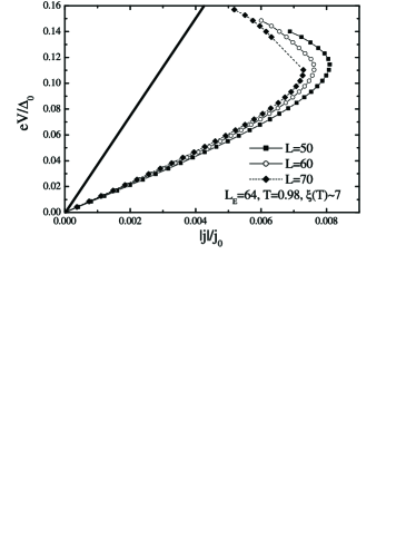
Figure 4: Current-voltage characteristics of the superconducting wire with relaxation length $L_{E}=64$, temperature $T=0.98$ and different wire lengths L (dashed line marks the voltage interval with no stationary solutions of Eqs. (1-3)). It demonstrates the absence of the stationary states at $V\sim V_{0}$ with increasing length of the wire.

For intermediate wire lengths $L\gg L_{E}\gg\xi(T)$ the situation is more complicated. At $V=V_{0}$ due to the suppression of the $|\Delta|$ near the edges by $f_{L}(E)$ the order parameter decays and the current decreases with increasing voltage. In Fig. 5 we show the spatial distribution of the order parameter for different values of the voltage for $L_{E}=64$ and $L_{E}=16$ (L=100, T=0.98). Due to the decay of $f_{L}$ on the scale $L_{E}$ and the term $\Psi_{1}$ in Eq. (3), the order parameter also starts to vary on a distance of about $L_{E}$. That’s why the order parameter is finite in a wider region of the wire with $L\sim L_{E}$ than for wires with $L\gg L_{E}$ even at $V\sim V_{c}$. The suppression of $|\Delta|$ near the ends of the short wire (with respect to $L_{E}$) is mainly connected with the relaxation of $f_{L}(E)$ due to the coupling with the transverse mode in Eq. (2a) (see discussion below).

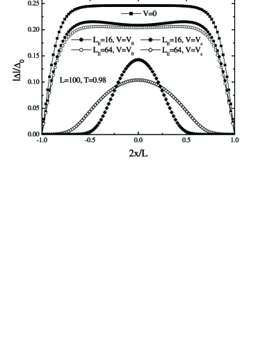
Figure 5: Distribution of the order parameter in a superconducting wire of length $L=100$ being in the symmetric superconducting state at different values of the applied voltage and relaxation lengths $L_{E}$.

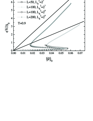
Figure 6: Current-voltage characteristics of the superconducting wires of different lengths and electron-phonon relaxation time (solid curves correspond to the normal state of the wires with lengths $L=100$ and $L=200$). It shows, that for a fixed temperature (not too close to $T_{c}$ in order to satisfy the condition $L_{E}\gg\xi(T)$) and relaxation length $L_{E}$ it is possible to find the length of the sample for which the IV characteristic will have a pronounced S-behavior.

When the region of the suppression of $|\Delta|$ increases up to about $L_{E}$ the effect of the nonequlibrium $f_{L}(E)$ becomes less pronounced, $|\Delta|$ decreases much slower with increasing voltage and the current starts to increase again. At some moment it reaches a value close to the depairing current density in the center of the wire and the state with a nonequlibrium and a stationary distribution of the order parameter becomes unstable ours2 . Phase slip centers should appear in the wire. This is observed as the absence of a stationary solution to Eqs. (1-3) in some range of applied voltage (marked dashed lines in Fig. 1(b)). With further increasing voltage the superconducting region decreases and we find again a stationary solution. At this voltage, the size of the superconducting region is too small to ’carry’ a phase slip state and is close to the critical size $10\xi(T)$ found above for the stability of the stationary state in the wire with $L_{E}\sim L$. The above mechanism leads to a S-shape for the IV characteristics for the intermediate case $L\gg L_{E}\gg\xi(T)$. This feature is more visible if we consider low temperatures and study samples of different lengths (see Fig. 6).

The relaxation of $f_{L}(E)$ and $f_{T}(E)$ to equilibrium occurs not only via the inelastic electron-phonon interaction but also due to the coupling terms $2DN_{2}R_{2}\nabla\varphi\nabla f_{T,L}$ in Eqs. (2a,b). They are nonzero in the region where the order parameter changes near the N-S border and where $\nabla f_{T,L}\neq 0$. This mechanism effectively relaxes the nonequilibrium $f_{L,T}(E)$ at energies close to $|\Delta|$ (where the product $N_{2}R_{2}\neq 0$). In Fig. 7 we present the spatial dependence of $f_{L}(E,x)-f_{L}^{0}(E)$ and $f_{T}(E,x)$ for different values of the energy for a wire with length L=100, temperature T=0.98, relaxation length $L_{E}=64$, applied voltage $V=0.08$ and with zero and nonzero coupling terms $2DN_{2}R_{2}\nabla\varphi\nabla f_{T,L}$ in Eq. (2). We notice that for energies close to $|\Delta|$ the coupling of the longitudinal mode with the transverse one leads even to a change in sign of $f_{L}(E)$ in the central part of the sample and hence to a smaller value of the term $\Psi_{1}$ in Eq. (3). The change of the relaxation length of the transverse mode $f_{T}$ is not so pronounced, but is still noticeable and justifies the faster decay due to coupling with the longitudinal mode.

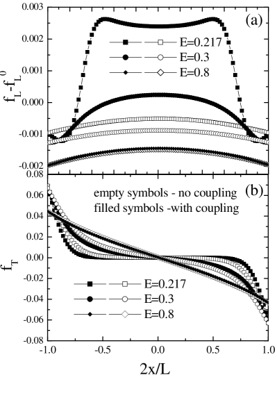
Figure 7: Spatial dependence of $f_{L}-f_{L}^{0}$ (a) and $f_{T}$ (b) at different energies for zero and nonzero coupling terms $2N_{2}R_{2}\nabla\varphi\nabla f_{L,T}$ in Eqs. (2a,b). Parameters of the wire: L=100, $L_{E}^{2}=2^{9}$, $T=0.98$, $V=0.08$, $\Delta(x=0,V=0.08)\simeq 0.216$.

That effect provides the dependence of the shape of the current-voltage characteristic of the wire on temperature (see Fig. 8) for fixed length of the sample and strength of the electron-phonon interaction even when $L\gg L_{E}>\xi(T)$. Above discussed additional mechanism of relaxation effectively shortens the relaxation length of $f_{L,T}(E)$ for $V\gtrsim V_{0}$ and decreases the effect of nonequilibrium when $L_{E}$ approaches $\xi(T)$. It moves the wire from the limit $L\gg L_{E}\gg\xi(T)$ to the limit $L\gg L_{E}\sim\xi(T)$ at some temperature close to $T_{c}$.

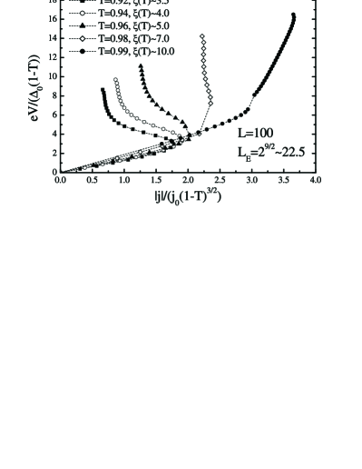
Figure 8: Current-voltage characteristics of the superconducting wire of fixed length and strength of the electron-phonon interaction for different temperatures. It shows the change of the shape of the IV characteristic when $L_{E}$ approaches $\xi(T)$.

IV Asymmetric states

To understand the origin of the asymmetric states in a superconducting wire let us consider as a example the mesoscopic normal metal wire half of which has a resistance larger than the other half. Applying a voltage to such a sample the voltage drop in the high resistance part will be larger than in the low resistance part (for definition we suppose that $R_{left}>R_{right}$) in order to satisfy the continuity of the current along the wire, i.e. $I(x)={\rm const}$. It means that if we put V=0 in the center of our inhomogeneous wire we have $|V(-L/2)|>|V(L/2)|$. Hence the deviation of the quasiparticle distribution functions from equilibrium in the left and right normal reservoirs ($f(E,x\pm L/2)-1/(\exp(E/T)+1)$) will depend not only on the value of the applied voltage but also on the properties of the mesoscopic wire.

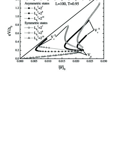
Figure 9: Current-voltage characteristics of the symmetric (empty symbols) and asymmetric (filled symbols) states. Solid curve shows the normal state. Dashed curves mark regions of absence of the stationary symmetric states. The stationary asymmetric state does not exist for $V<V_{0}$ - voltage where negative-differential resistance appears for symmetric state.

To find corresponding superconducting state in our homogeneous system we use the asymmetric boundary conditions $V(\pm L/2)=\mp V+dV$. The addition dV is determined from the condition of constant current along the wire. It increases from zero (at $V\simeq V_{0}$) to a finite value (at $V_{c}^{a}$ - critical voltage of the asymmetric state). No asymmetric states were found for $V<V_{0}$. In Fig. 9 we show typical IV characteristics and in Fig. 10 we present the corresponding distribution of the order parameter for symmetric and asymmetric states at the same values of the voltage. It is obvious from the above discussion that the order parameter is more suppressed on the side of the wire with maximal absolute value of the voltage. For example if we change the sign of dV the order parameter distribution in Fig. 10 will be symmetrically reflected with respect to x=0.

It is interesting to note that such an asymmetric state may exist up to larger values of the voltage when $L\gtrsim L_{E}\gg\xi$, and even for larger values of the current, than the symmetric state (latter property is realized for lengths $L\sim L_{E}$ for which the IV characteristic changes slope from a negative to a positive one for the symmetric state when $V>V_{0}$). Another interesting property is the existence of the stationary asymmetric state for voltages when the stationary symmetric state is absent (see Fig. 9).

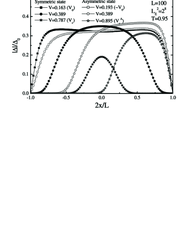
Figure 10: Order parameter distribution for asymmetric and symmetric states.

The range of the existence of the stationary asymmetric state is rather small in comparison with the symmetric state when the length of the wire is much larger than $L_{E}$. It exists only at voltages near $V_{0}$ (see Figs. 9 and 11 for small ratios $L_{E}/L$).

We did not find stationary asymmetric states for wires with $L_{E}\sim\xi(T)$. For small values $L_{E}\ll\xi(T)$ the asymmetric state is nearly the same as the symmetric one but shifted with respect to the point $x=0$ and the IV characteristics are found to be nearly the same for both symmetric and asymmetric states. This is explained by the negligible effect of $f_{L}(E)$ on the value of the order parameter in this limit.

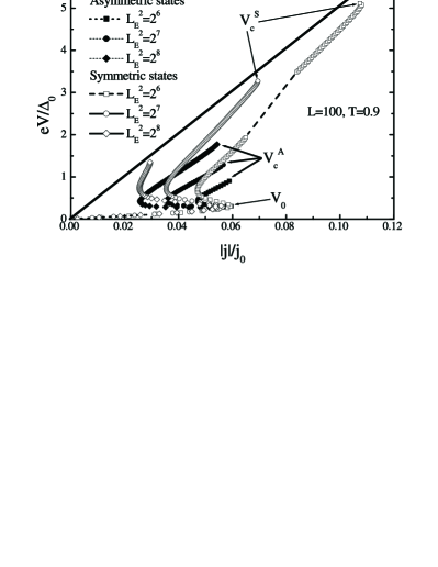
Figure 11: Current-voltage characteristics for symmetric and asymmetric states for wires with different $L_{E}$.

V Conclusion

The response of a dirty superconducting wire that is connected to normal metal banks, to an applied voltage, strongly depends on the ratio between the length of the sample $L$, the coherence length $\xi$ and relaxation length $\overline{L_{E}}$ of the nonequilibrium quasiparticle distribution function $f(E)$. The latter one, was determined in our calculations by the inelastic electron-phonon interaction $\overline{L_{E}}=\sqrt{D\tau_{E}}$ with an energy independent characteristic time $\tau_{E}$. Applied voltage suppresses the superconducting order parameter both via the creation of the superconducting current and the modification of the quasiparticle distribution function. First mechanism is prevalent when $L_{E}\lesssim\xi(T)$ and the second one is dominant in the opposite limit $L_{E}\gg\xi(T)$ for samples with $L\sim L_{E}$. For wires with $L\gg L_{E}\gg\xi(T)$ the transition to the normal state is mainly induced by the superconducting current.

We found that for the following two cases $L\gg\xi(T)>L_{E}$ and $L\gtrsim L_{E}\gg\xi(T)$ there are three stationary solutions to Eqs. (1-3) at given value of the applied voltage difference $2V>2V_{0}$ - one symmetric state and two asymmetric states (which are symmetrically reflected to the center of the wire) which are characterized by symmetric and asymmetric distribution of the order parameter, respectively. The degeneracy is most pronounced in the limit $L\gtrsim L_{E}\gg\xi(T)$ because the order parameter may vary on the distance of order $L_{E}\gg\xi$ due to the long relaxation length of the odd (in energy) part of the nonequilibrium quasiparticle distribution function and it provides the basis for the appearance of new effects. For example it leads to an S-behavior of the IV characteristic of the wire being in the symmetric state. In the same limit the stationary asymmetric state may exist even when the symmetric one exist only as a time-dependent one (phase slip state) (see Fig. 9). Moreover, for a specific temperature and length $L_{E}\gg\xi(T)$ there exist length of the sample for which a stationary asymmetric state does exist up to a larger value of the current than the stationary symmetric one (see Fig. 9 and compare for $L_{E}^{2}=2^{8}$).

We should mention here, that in the extended TDGL equation there is no direct effect of the voltage on the value of the order parameter. This is because of the ”local equilibrium approximation” (valid in the limit $L_{E}\ll\xi(T)$) Kramer ; Watts-Tobin where it was assumed that $f_{L}-f_{L}^{0}$ is only proportional to the time variation of the value of the order parameter $\partial|\Delta|/\partial t$ and hence is zero in the stationary case. But it is interesting to note that the asymmetric state could also be obtained by this equation. For example the asymmetric state exists for $\gamma=32,L=100,T=0.98$ (see inset in Fig. 1a) at $0.217<V<0.242$. But we did not find in this model the wire parameters for which asymmetric and symmetric states could exist at the same value of the voltage.

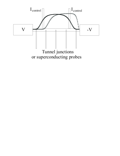
Figure 12: Proposed experimental setup to measure transitions between symmetric and asymmetric states and current-voltage characteristic of both states. The curves with empty and filled symbols show the order parameter distribution for a wire with parameters from Fig. 10 and V=0.389.

Experimentally the asymmetric state may be realized by adding additional contacts to the superconducting wire with control current close to the ends of the wire (see Fig. 10). It is better to contact the wire with the reservoirs made from the same material and to apply a strong enough magnetic field to suppress the superconductivity in the reservoirs. This procedure will provide good contact with normal reservoirs. Applying strong enough current to only one of the current contacts we locally destroy superconductivity and force an asymmetric distribution of the order parameter. After switching off the control current the asymmetric distribution should be stable (at proper choice of the working point at the IV characteristic). To come back to the symmetric state we should apply a control current at the both current contacts and it will force the recovering the symmetric state in the wire. We will need a series of tunnel junctions along the wire to measure locally the strength of the order parameter. Other alternative is to use superconducting (SC) probes to distinguish the part of the superconductor with attached SC-probe in the normal or superconducting state. When in the normal state the superconducting probe measures the electrostatic potential.

Good candidates to observe these symmetric and asymmetric states is dirty aluminium and zinc with their relatively large coherence lengths ($\xi_{Al}(0)\sim 0.15\mu m$, $\xi_{Zn}(0)\sim 0.25\mu m$ ) and $\overline{L_{E}}(Al)\sim 9\mu m$, $\overline{L_{E}}(Zn)\sim 35\mu m$ ($L_{E}(Al)\sim 60$, $L_{E}(Zn)\sim 140$). The expected temperature range for the validity of our results is $0.9<T/T_{c}<1$. The most strict restriction to observe these effects is that there should be only a small heating of the sample. Heating will initiate the transition of the sample to the normal state and hide the main effects.

For other low-temperature superconductors (Nb, Pb, In, Sn) we have $L_{E}<10$ (we used data for $\tau_{E}$ at $T\sim T_{c}$ from Ref. Stuivinga ). It means that at $T\geq 0.9$ the coherence length is comparable with $L_{E}$. For these conditions we did not find asymmetric states. Moreover the effect of nonequilibrium in the odd part of the quasiparticle distribution function that is connected with the applied voltage is rather small for these parameters and the extended TDGL equations gives result which are qualitatively similar to the one obtained here.

- (1) C. C. Chi and J. Clarke, Phys. Rev. B 20, 4465 (1979).
- (2) M. G. Blamire, E. C. G. Kirk, J.E. Evetts, and T. M. Klapwijk, Phys. Rev. Lett. 66, 220 (1991).
- (3) J. Clarke, in: Nonequlibrium superconductivity, edited by D.N. Langenberg and A.I. Larkin, (Elsevier Science Publisher B.V., Berlin, 1986), p. 1 and references therein.
- (4) V. M. Dmitriev, V. N. Gubankov and F. Ya. Nad’, in: Nonequlibrium superconductivity, edited by D.N. Langenberg and A.I. Larkin, (Elsevier Science Publisher B.V., Berlin, 1986), p. 163 and references therein.
- (5) G. M. Eliashberg and B. I. Ivlev, in: Nonequlibrium superconductivity, edited by D.N. Langenberg and A.I. Larkin, (Elsevier Science Publisher B.V., Berlin, 1986), p. 211 and references therein.
- (6) A.I. Larkin and Yu. N. Ovchinnikov, in: Nonequlibrium superconductivity, edited by D.N. Langenberg and A.I. Larkin, (Elsevier Science Publisher B.V., Berlin, 1986), p. 493 and references therein.
- (7) M. Tinkham, Introduction to superconductivity, (McGraw-Hill, NY, 1996).
- (8) R. S. Keizer, M. G. Flokstra, J. Aarts, and T. M. Klapwijk, Phys. Rev. Lett. 96, 147002 (2006).
- (9) K. D. Usadel, Phys. Rev. Lett. 25, 507 (1970).
- (10) A. Schmid and G. Schön, J. Low Temp. Phys. 20, 207 (1975).
- (11) L. Kramer and R.J. Watts-Tobin, Phys. Rev. Lett. 40, 1041 (1978).
- (12) R.J. Watts-Tobin, Y. Krähenbühl, and L. Kramer, J. Low Temp. Phys. 42, 459 (1981).
- (13) D. Y. Vodolazov, A. Elmurodov, and F. M. Peeters, Phys. Rev. B 72, 134509 (2005).
- (14) We found that for there exist two solutions to Eq. (7). Because we are not interested in this temperature interval we did not investigate this phenomena in detail.
- (15) Here we should mention that for relatively large relaxation length the critical current for the stability of the N-S border is larger than the depairing current density and superconductivity becomes unstable in the center of the wire. The reason is that the superconducting current (not the whole current) destroys superconductivity, but it is small at the N-S border for large .
- (16) M. Stuivinga, J. E. Mooij, and T. M. Klapwijk, J. Low Temp. Phys. 46, 555 (1982).