Phase separation of a driven granular gas in annular geometry

Abstract

This work investigates phase separation of a monodisperse gas of inelastically colliding hard disks confined in a two-dimensional annulus, the inner circle of which represents a “thermal wall”. When described by granular hydrodynamic equations, the basic steady state of this system is an azimuthally symmetric state of increased particle density at the exterior circle of the annulus. When the inelastic energy loss is sufficiently large, hydrodynamics predicts spontaneous symmetry breaking of the annular state, analogous to the van der Waals-like phase separation phenomenon previously found in a driven granular gas in rectangular geometry. At a fixed aspect ratio of the annulus, the phase separation involves a “spinodal interval” of particle area fractions, where the gas has negative compressibility in the azimuthal direction. The heat conduction in the azimuthal direction tends to suppress the instability, as corroborated by a marginal stability analysis of the basic steady state with respect to small perturbations. To test and complement our theoretical predictions we performed event-driven molecular dynamics (MD) simulations of this system. We clearly identify the transition to phase separated states in the MD simulations, despite large fluctuations present, by measuring the probability distribution of the amplitude of the fundamental Fourier mode of the azimuthal spectrum of the particle density. We find that the instability region, predicted from hydrodynamics, is always located within the phase separation region observed in the MD simulations. This implies the presence of a binodal (coexistence) region, where the annular state is metastable. The phase separation persists when the driving and elastic walls are interchanged, and also when the elastic wall is replaced by weakly inelastic one.

I Introduction

Flows of granular materials are ubiquitous in nature and technology jaeger . Examples are numerous and range from Saturn’s rings to powder processing. Being dissipative and therefore intrinsically far from thermal equilibrium, granular flows exhibit a plethora of pattern forming instabilities ristow ; aranson+tsimring . In spite of a surge of recent interest in granular flows, their quantitative modeling remains challenging, and the pattern forming instabilities provide sensitive tests to the models. This work focuses on the simple model of rapid granular flows, also referred to as granular gases: large assemblies of inelastically colliding hard spheres campbell ; kadanoff ; thorsten1 ; thorsten2 ; goldhirsch1 ; brilliantov . In the simplest version of this model the only dissipative effect taken into account is a reduction in the relative normal velocity of the two colliding particles, modeled by the coefficient of normal restitution, see below. Under some additional assumptions a hydrodynamic description of granular gases becomes possible. The Molecular Chaos assumption allows for a description in terms of the Boltzmann or Enskog equations, properly generalized to account for the inelasticity of particle collisions, followed by a systematic derivation of hydrodynamic equations sela ; brey1 ; lutsko . For inhomogeneous (and/or unsteady) flows hydrodynamics demands scale separation: the mean free path of the particles (respectively, the mean time between two consecutive collisions) must be much less than any characteristic length (respectively, time) scale that the hydrodynamic theory attempts to describe. The implications of these conditions can be usually seen only a posteriori, after the hydrodynamic problem in question is solved, and the hydrodynamic length/time scales are determined. We will restrict ourselves in this work to nearly elastic collisions and moderate gas densities where, based on previous studies, hydrodynamics is expected to be an accurate leading order theory campbell ; kadanoff ; thorsten1 ; thorsten2 ; goldhirsch1 ; brilliantov . These assumptions allow for a detailed quantitative study (and prediction) of a variety of pattern formation phenomena in granular gases. One of these phenomena is the phase separation instability, first predicted in Ref. livne1 and further investigated in Refs. argentina ; brey2 ; khain1 ; livne2 ; baruch2 ; khain2 . This instability arises already in a very simple, indeed prototypical setting: a monodisperse granular gas at zero gravity confined in a rectangular box, one of the walls of which is a “thermal” wall. The basic state of this system is the stripe state. In the hydrodynamic language it represents a laterally uniform stripe of increased particle density at the wall opposite to the driving wall. The stripe state was observed in experiment kudrolli , and this and similar settings have served for testing the validity of quantitative modeling kadanoff2 ; esipov ; grossman . It turns out that (i) within a “spinodal” interval of area fractions and (ii) if the system is sufficiently wide in the lateral direction, the stripe state is unstable with respect to small density perturbations in the lateral direction livne1 ; brey2 ; khain1 . Within a broader “binodal” (or coexistence) interval the stripe state is stable to small perturbations, but unstable to sufficiently large ones argentina ; khain2 . In both cases the stripe gives way, usually via a coarsening process, to coexistence of dense and dilute regions of the granulate (granular “droplets” and “bubbles”) along the wall opposite to the driving wall argentina ; livne2 ; khain2 . This far-from-equilibrium phase separation phenomenon is strikingly similar to a gas-liquid transition as described by the classical van der Waals model, except for large fluctuations observed in a broad region of aspect ratios around the instability threshold baruch2 . The large fluctuations have not yet received a theoretical explanation.

This work addresses a phase separation process in a different geometry. We will deal here with an assembly of hard disks at zero gravity, colliding inelastically inside a two-dimensional annulus. The interior wall of the annulus drives the granulate into a non-equilibrium steady state with a (hydrodynamically) zero mean flow. Particle collisions with the exterior wall are assumed elastic. The basic steady state of this system, as predicted by hydrodynamics, is the annular state: an azimuthally symmetric state of increased particle density at the exterior wall. The phase separation instability manifests itself here in the appearance of dense clusters with broken azimuthal symmetry along the exterior wall. Our main objectives are to characterize the instability and compute the phase diagram by using granular hydrodynamics (or, more precisely, granular hydrostatics, see below) and event driven molecular dynamics simulations. By focusing on the annular geometry, we hope to motivate experimental studies of the granular phase separation which may be advantageous in this geometry. The annular setting avoids lateral side walls (with an unnecessary/unaccounted for energy loss of the particles). Furthermore, driving can be implemented here by a rapid rotation of the (slightly eccentric and possibly rough) interior circle.

We organized the paper as follows. Section II deals with a hydrodynamic description of the annular state of the gas. As we will be dealing only with states with a zero mean flow, we will call the respective equations hydrostatic. A marginal stability analysis predicts a spontaneous symmetry breaking of the annular state. We compute the marginal stability curves and compare them to the borders of the spinodal (negative compressibility) interval of the system. In Section III we report event-driven molecular dynamics (MD) simulations of this system and compare the simulation results with the hydrostatic theory. In Section IV we discuss some modifications of the model, while Section V contains a summary of our results.

II Particles in an annulus and granular hydrostatics

The density equation. Let $N$ hard disks of diameter $d$ and mass $m=1$ move, at zero gravity, inside an annulus of aspect ratio $\Omega=R_{\text{ext}}/R_{\text{int}}$, where $R_{\text{ext}}$ is the exterior radius and $R_{\text{int}}$ is the interior one. The disks undergo inelastic collisions with a constant coefficient of normal restitution $\mu$. For simplicity, we neglect the rotational degree of freedom of the particles. The (driving) interior wall is modeled by a thermal wall kept at temperature $T_{0}$, whereas particle collisions with the exterior wall are considered elastic. The energy transferred from the thermal wall to the granulate dissipates in the particle inelastic collisions, and we assume that the system reaches a (non-equilibrium) steady state with a zero mean flow. We restrict ourselves to the nearly elastic limit by assuming a restitution coefficient close to, but less than, unity: $1-\mu\ll 1$. This allows us to safely use granular hydrodynamics goldhirsch1 . For a zero mean flow steady state the continuity equation is obeyed trivially, while the momentum and energy equations yield two hydrostatic relations:

$$\nabla\cdot\mathbf{q}(\mathbf{r})+I=0\,,\;\;\;p=const\,,$$ (1)

where $\mathbf{q}$ is the local heat flux, $I$ is the energy loss term due to inelastic collisions, and $P=P(n,T)$ is the gas pressure that depends on the number density $n(\mathbf{r})$ and granular temperature $T(\mathbf{r})$. We adopt the classical Fourier relation for the heat flux $\mathbf{q}(\mathbf{r})=-\kappa\nabla T(\mathbf{r})$ (where $\kappa$ is the thermal conductivity), omitting a density gradient term. In the dilute limit this term was derived in Ref. brey1 . It can be neglected in the nearly elastic limit which is assumed throughout this paper.

The momentum and energy balance equations read

$$\nabla\cdot\left[\kappa\nabla T(\mathbf{r})\right]=I\,,\;\;\;p=const\,,$$ (2)

To get a closed formulation, we need constitutive relations for $p(n,T)$, $\kappa(n,T)$ and $I(n,T)$. We will employ the widely used semi-empiric transport coefficients derived by Jenkins and Richman jenkins for moderate densities:

$$\begin{split}\kappa=\frac{2dnT^{1/2}\tilde{G}}{\pi^{1/2}}\left[1+\frac{9\pi}{16}\left(1+\frac{2}{3\tilde{G}}\right)^{2}\right],\\ I=\frac{8(1-\mu)nT^{3/2}\tilde{G}}{d\sqrt{\pi}}\,,\end{split}$$ (3)

and the equation of state first proposed by Carnahan and Starling carnahan

$$p=nT(1+2\tilde{G})\,,$$ (4)

where $\tilde{G}=\nu(1-\frac{7\nu}{16})/(1-\nu)^{2}$ and $\nu=n\left(\pi d^{2}/4\right)$ is the solid fraction. Let us rescale the radial coordinate by $R_{\text{int}}$ and introduce the rescaled inverse density $Z(r,\theta)=n_{c}/n(r,\theta)$, where $n_{c}=2/\left(\sqrt{3}d^{2}\right)$ is the hexagonal close packing density. The rescaled radial coordinate $r$ now changes between $1$ and $\Omega\equiv R_{\text{ext}}/R_{\text{int}}$, the aspect ratio of the annulus. As in the previous work khain1 , Eqs. (2), (4) and (3) can be transformed into a single equation for the inverse density $Z(r)$:

$$\nabla\cdot\left[\mathcal{F}(Z)\nabla Z\right]=\Lambda\mathcal{Q}(Z)\,,$$ (5)

where

$$\begin{split}\mathcal{F}(Z)=\mathcal{F}_{1}(Z)\mathcal{F}_{2}(Z),\\ \mathcal{Q}(Z)=\frac{6}{\pi}\frac{Z^{1/2}\mathcal{G}}{(1+2\mathcal{G})^{3/2}},\\ \mathcal{F}_{1}(Z)=\frac{\mathcal{G}(Z)\left[1+{\frac{9\pi}{16}}\left(1+\frac{2}{3\mathcal{G}}\right)^{2}\right]}{Z^{1/2}(1+2\mathcal{G})^{5/2}},\\ \mathcal{F}_{2}(Z)=1+2\mathcal{G}+\frac{\pi}{\sqrt{3}}\frac{Z\left(Z+\frac{\pi}{16\sqrt{3}}\right)}{\left(Z-\frac{\pi}{2\sqrt{3}}\right)^{3}},\\ \mathcal{G}(Z)=\frac{\pi}{2\sqrt{3}}\frac{\left(Z-\frac{7\pi}{32\sqrt{3}}\right)}{\left(Z-\frac{\pi}{2\sqrt{3}}\right)^{2}}.\end{split}$$ (6)

The dimensionless parameter $\Lambda\equiv(2\pi/3)(1-\mu)\left(R_{\text{int}}/d\right)^{2}$ is the hydrodynamic inelastic loss parameter. The boundary conditions for Eq. (5) are

$$\partial Z(1,\theta)/\partial\theta=0\quad\text{and}\quad\nabla_{n}Z(\Omega,\theta)=0\,,$$ (7)

The first of these follows from the constancy of the temperature at the (thermal) interior wall which, in view of the constancy of the pressure in a steady state, becomes constancy of the density. The second condition demands a zero normal component of the heat flux at the elastic wall. Finally, working with a fixed number of particles, we demand the normalization condition

$$\int_{0}^{2\pi}\int_{1}^{\Omega}Z^{-1}(r,\theta)rdrd\theta=\pi f(\Omega^{2}-1)\,,$$ (8)

where

$$f=\frac{N}{\pi n_{c}R_{\text{int}}^{2}(\Omega^{2}-1)}$$

is the area fraction of the grains in the annulus. Equations (5)-(8) determine all possible steady state density profiles, governed by three dimensionless parameters: $f$, $\Lambda$, and $\Omega$.

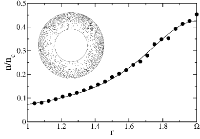
Figure 1: The normalized density profiles obtained from the MD simulations (the dots) and hydrostatics (the line) for $\Omega=2$, $\Lambda=81.09$, and $f=0.356$ (equivalently, $z_{\Omega}=2.351$). The simulations were carried out with $N=1250$ particles, $\mu=0.92$, and $R_{\text{int}}=22.0$. Also shown is a typical snapshot of the system at the steady state as observed in the MD simulation.

Annular state. The simplest solution of the density equation (5) is azimuthally symmetric ($\theta$-independent): $Z=z(r)$. Henceforth we refer to this basic state of the system as the annular state. It is determined by the following equations:

$$\begin{split}\left[r\mathcal{F}(z)z^{\prime}\right]^{\prime}=r\Lambda\mathcal{Q}(z),\;z^{\prime}(\Omega)=0,\;\text{and}\\ \int_{1}^{\Omega}z^{-1}rdr=(\Omega^{2}-1)f/2\,,\end{split}$$ (9)

where the primes denote $r$-derivatives. In order to solve the second order equation (9) numerically, one can prescribe the inverse density at the elastic wall $z_{\Omega}\equiv z(\Omega)$. Combined with the no-flux condition at $r=\Omega$, this condition define a Cauchy problem for $z(r)$ livne2 ; khain1 . Solving the Cauchy problem, one can compute the respective value of $f$ from the normalization condition in Eq. (9). At fixed $\Lambda$ and $\Omega$, there is a one-to-one relation between $z_{\Omega}$ and $f$. Therefore, an alternative parameterization of the annular state is given by the scaled numbers $z_{\Omega}$, $\Lambda$, and $\Omega$. The same is true for the marginal stability analysis performed in the next subsection.

Figure 1 depicts an example of annular state that we found numerically. One can see that the gas density increases with the radial coordinate, as expected from the temperature decrease via inelastic losses, combined with the constancy of the pressure throughout the system. The hydrodynamic density profile agrees well with the one found in our MD simulations, see below.

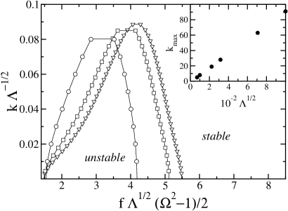
Figure 2: The main graph: the marginal stability curves $k=k(f)$ (where $k$ is an integer) for $\Omega=1.5$ and $\Lambda=10^{4}$ (circles), $\Lambda=5\times 10^{4}$ (squares), and $\Lambda=10^{5}$ (triangles). For a given $\Lambda$ the annular state is stable above the respective curve and unstable below it, as indicated for $\Lambda=10^{4}$. As $\Lambda$ increases the marginal stability interval shrinks. The inset: the dependence of $k_{max}$ on $\Lambda^{1/2}$. The straight line shows that, at large $\Lambda$, $k_{max}\propto\Lambda^{1/2}$.

Phase separation. Mathematically, phase separation manifests itself in the existence of additional solutions to Eqs. (5)-(8) in some region of the parameter space $f$, $\Lambda$, and $\Omega$. These additional solutions are not azimuthally symmetric. Solving Eqs. (5)-(8) for fully two-dimensional solutions is not easy livne1 . One class of such solutions, however, bifurcate continuously from the annular state, so they can be found by linearizing Eq. (5), as in rectangular geometry livne1 ; khain1 . In the framework of a time-dependent hydrodynamic formulation, this analysis corresponds to a marginal stability analysis which involves a small perturbation to the annular state. For a single azimuthal mode $\sim\sin(k\theta)$ (where $k$ is integer) we can write $Z(r,\theta)=z(r)+\varepsilon\;\Xi(r)\sin(k\theta)$, where $\Xi(r)$ is a smooth function, and $\varepsilon\ll 1$ a small parameter. Substituting this into Eq. (5) and linearizing the resulting equation yields a $k$-dependent second order differential equation for the function $\Gamma(r)\equiv\mathcal{F}[Z(r)]\,\Xi(r)$:

$$\Gamma^{\prime\prime}_{k}+\frac{1}{r}\Gamma^{\prime}_{k}-\left(\frac{k^{2}}{r^{2}}+\frac{\Lambda\mathcal{Q}^{\prime}(Z)}{\mathcal{F}(Z)}\right)\Gamma_{k}=0\,.$$ (10)

This equation is complemented by the boundary conditions

$$\Gamma(1)=0\;\;\;\mbox{and}\;\;\;\Gamma^{\prime}(\Omega)=0\,.$$ (11)

For fixed values of the scaled parameters $f$, $\Lambda$, and $\Omega$, Eqs. (10) and (11) determine a linear eigenvalue problem for $k$. Solving this eigenvalue problem numerically, one obtains the marginal stability hypersurface $k=k(f,\Lambda,\Omega)$. For fixed $\Lambda$ and $\Omega$, we obtain a marginal stability curve $k=k(f)$. Examples of such curves, for a fixed $\Omega$ and three different $\Lambda$ are shown in Fig. 2. Each $k=k(f)$ curve has a maximum $k_{max}$, so that a density modulation with the azimuthal wavenumber larger than $k_{max}$ is stable. As expected, the instability interval is the largest for the fundamental mode $k=1$. The inset in Fig. 2 shows the dependence of $k_{max}$ on $\Lambda^{1/2}$. The straight line shows that, at large $\Lambda$, $k_{max}\propto\Lambda^{1/2}$, as in rectangular geometry khain1 .

Two-dimensional projections of the ($f$, $\Lambda$, $\Omega$)-phase diagram at three different $\Omega$ are shown in Fig. 3 for the fundamental mode. The annular state is unstable in the region bounded by the marginal stability curve, and stable elsewhere. Therefore, the marginal stability analysis predicts loss of stability of the annular state within a finite interval of $f$, that is at $f_{min}(\Lambda,\Omega)<f<f_{max}(\Lambda,\Omega)$.

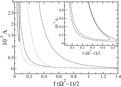
Figure 3: Two-dimensional projections on the $[\Lambda$, $f\,(\Omega^{2}-1)/2]$ plane of the phase diagram at $\Omega=1.5$ (the solid line), $\Omega=3$ (the dotted line), and $\Omega=5$ (the dashed line). The inset shows more clearly, for $\Omega=3$, that the marginal stability curve (the solid line) lies within the negative compressibility region (bounded by the dashed line).

The physical mechanism of this phase separation instability is the negative compressibility of the granular gas in the azimuthal direction, caused by the inelastic energy loss. To clarify this point, let us compute the pressure of the annular state, given by Eq. (4). First we introduce a rescaled pressure $P=p/(n_{c}T_{0})$ and, in view of the pressure constancy in the annular state, compute it at the thermal wall, where $T=T_{0}$ is prescribed and $z(1)$ is known from our numerical solution for the annular state. We obtain

$$P(f,\Lambda,\Omega)=\frac{1+2\mathcal{G}(z(1))}{z(1)}\,.$$

The spinodal (negative compressibility) region is determined by the necessary condition for the instability: $\left(\partial P/\partial f\right)_{\Lambda,\Omega}<0$, whereas the borders of the spinodal region are defined by $\left(\partial P/\partial f\right)_{\Lambda,\Omega}=0$. Typical $P(f)$ curves for a fixed $\Omega$ and several different $\Lambda$ are shown in Fig. 4. One can see that, at sufficiently large $\Lambda$, the rescaled pressure $P$ goes down with an increase of $f$ at an interval $f_{1}<f<f_{2}$. That is, the effective compressibility of the gas with respect to a redistribution of the material in the azimuthal direction is negative on this interval of area fractions. By joining the spinodal points $f_{1}$ and (separately) $f_{2}$ at different $\Lambda$, we can draw the spinodal line for a fixed $\Omega$. As $\Lambda$ goes down, the spinodal interval shrinks and eventually becomes a point at a critical point $(P_{c},f_{c})$, or $(\Lambda_{c},f_{c})$ (where all the critical values are $\Omega$-dependent). For $\Lambda<\Lambda_{c}$ $P(f)$ monotonically increases and there is no instability.

What is the relation between the spinodal interval $(f_{1},f_{2})$ and the marginal stability interval $(f_{min},f_{max})$? These intervals would coincide were the azimuthal wavelength of the perturbation infinite (or, equivalently, $k\rightarrow 0$), so that the azimuthal heat conduction would vanish. Of course, this is not possible in annular geometry, where $k\geq 1$. As a result, the negative compressibility interval must include in itself the marginal stability interval $(f_{min},f_{max})$. This is what our calculations indeed show, see the inset of Fig. 3. That is, a negative compressibility is necessary, but not sufficient, for instability, similarly to what was found in rectangular geometry khain1 .

Importantly, the instability region of the parameter space is by no means not the whole region the region where phase separation is expected to occur. Indeed, in analogy to what happens in rectangular geometry argentina ; khain2 , phase separation is also expected in a binodal (or coexistence) region of the area fractions, where the annular state is stable to small perturbations, but unstable to sufficiently large ones. The whole region of phase separation should be larger than the instability region, and it should of course include the instability region. Though we did not attempt to determine the binodal region of the system from the hydrostatic equations (this task has not been accomplished yet even for rectangular geometry, except in the close vicinity of the critical point khain2 ), we determined the binodal region from our MD simulations reported in the next section.

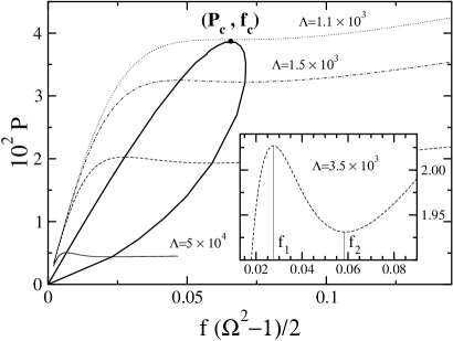
Figure 4: The scaled steady state granular pressure $P$ versus the grain area fraction $f$ for $\Omega=1.5$ and $\Lambda=1.1\times 10^{3}$ (the dotted line), $\Lambda=1.5\times 10^{3}$ (the dash-dotted line), $\Lambda=3.5\times 10^{3}$ (dashed line), and $\Lambda=5\times 10^{4}$ (the solid line). The inset shows a zoom-in for $\Lambda=3.5\times 10^{3}$. The borders $f_{1}$ and $f_{2}$ of the spinodal interval are determined from the condition $\left(\partial P/\partial f\right)_{\Lambda,\Omega}=0$. The thick solid line encloses the spinodal balloon where the effective azimuthal compressibility of the gas is negative.

III MD Simulations

Method. We performed a series of event-driven MD simulations of this system using an algorithm described by Pöschel and Schwager thorsten3 . Simulations involved $N$ hard disks of diameter $d=1$ and mass $m=1$. After each collision of particle $i$ with particle $j$, their relative velocity is updated according to

$$\vec{v}_{ij}^{\,\prime}=\vec{v}_{ij}-\left(1+\mu\right)\left(\vec{v}_{ij}\cdot\hat{r}_{ij}\right)\hat{r}_{ij}\,,$$ (12)

where $\vec{v}_{ij}$ is the precollisional relative velocity, and $\hat{r}_{ij}\equiv\vec{r}_{ij}/\left|\vec{r}_{ij}\right|$ is a unit vector connecting the centers of the two particles. Particle collisions with the exterior wall $r=R_{\text{ext}}$ are assumed elastic. The interior wall is kept at constant temperature $T_{0}$ that we set to unity. This is implemented as follows. When a particle collides with the wall it forgets its velocity and picks up a new one from a proper Maxwellian distribution with temperature $T_{0}$, see e.g. Ref. thorsten3 , pages 173-177, for detail. The time scale is therefore $d(m/T_{0})^{1/2}=1$. The initial condition is a uniform distribution of non-overlapping particles inside the annular box. Their initial velocities are taken randomly from a Maxwellian distribution at temperature $T_{0}=1$. In all simulations the coefficient of normal restitution $\mu=0.92$ and the interior radius $R_{\text{int}}/d=22.0$ were fixed, whereas the the number of particles $527\leq N\leq 7800$ and the aspect ratio $1.5\leq\Omega\leq 6$ were varied. In terms of the three scaled hydrodynamic parameters the heat loss parameter $\Lambda=81.09$ was fixed whereas $f$ and $\Omega$ varied.

To compare the simulation results with predictions of our hydrostatic theory, all the measurements were performed once the system reached a steady state. This was monitored by the evolution of the total kinetic energy $(1/2)\sum_{i=1}^{N}\vec{v}_{i}^{\;2}$, which first decays and then, on the average, stays constant.

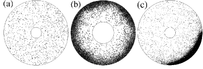
Figure 5: Typical steady state snapshots for $N=1250$ and $\Omega=6$ (a); $N=5267$ and $\Omega=3$ (b), and $N=6320$ and $\Omega=6$ (c). Panels (a) and (b) correspond to annular states of the hydrostatic theory, whereas panel (c) shows a broken-symmetry (phase separated) state.

Steady States. Typical steady state snapshots of the system, observed in our MD simulation, are displayed in Fig. 5. Panel (a) shows a dilute state where the radial density inhomogeneity, though actually present, is not visible by naked eye. Panels (b) and (c) do exhibit a pronounced radial density inhomogeneity. Apart from visible density fluctuations, panels (a) and (b) correspond to annular states. Panel (c) depicts a broken-symmetry (phase separated) state. When an annular state is observed, its density profile agrees well with the solution of the hydrostatic equations (5)-(8). A typical example of such a comparison is shown in Fig. 1.

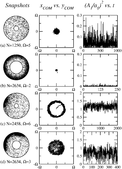
Figure 6: Typical steady state snapshots (the left column) and the temporal evolution of the COM (the middle column) and of the squared amplitude of the fundamental Fourier mode (the right column). The temporal data are sampled each $150$ collisions per particle. Each row corresponds to one simulation with the indicated parameters. The vertical scale of panels a and b was stretched for clarity.

Let us fix the aspect ratio $\Omega$ of the annulus at not too a small value and vary the number of particles $N$. First, what happens on a qualitative level? The simulations show that, at small $N$, dilute annular states, similar to snapshot (a) in Fig. 5, are observed. As $N$ increases, broken-symmetric states start to appear. Well within the unstable region, found from hydrodynamics, a high density cluster appears, like the one shown in Fig. 5c, and performs an erratic motion along the exterior wall. As $N$ is increased still further, well beyond the high-$f$ branch of the unstable region, an annular state reappears, as in Fig. 5b. This time, however, the annular state is denser, while its local structure varies from a solid-like (with imperfections such as voids and line defects) to a liquid-like.

To characterize the spatio-temporal behavior of the granulate at a steady state, we followed the position of the center of mass (COM) of the granulate. Several examples of the COM trajectories are displayed in Fig. 6. Here cases (a) and (b) correspond, in the hydrodynamic language, to annular states. There are, however, significant fluctuations of the COM around the center of the annulus. These fluctuations are of course not accounted for by hydrodynamic theory. In case (b), where the dense cluster develops, the fluctuations are much weaker that in case (a). More interesting are cases (c) and (d). They correspond to broken-symmetry states: well within the phase separation region of the parameter space (case c) and close to the phase separation border (case d). The COM trajectory in case (c) shows that the granular “droplet” performs random motion in the azimuthal direction, staying close to the exterior wall. This is in contrast with case (d), where fluctuations are strong both in the azimuthal and in the radial directions. Following the actual snapshots of the simulation, one observes here a very complicated motion of the “droplet”, as well as its dissolution into more “droplets”, mergers of the droplets etc. Therefore, as in the case of granular phase separation in rectangular geometry baruch2 , the granular phase separation in annular geometry is accompanied by considerable spatio-temporal fluctuations. In this situation a clear distinction between a phase-separated state and an annular state, and a comparison between the MD simulations and hydrodynamic theory, demand proper diagnostics. We found that such diagnostics are provided by the azimuthal spectrum of the particle density and its probability distribution.

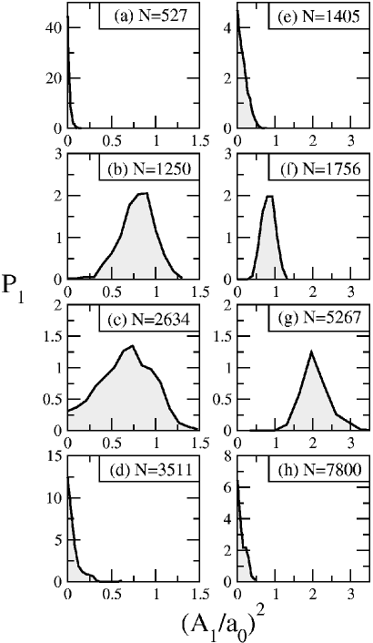
Figure 7: The normalized probability distribution functions $P_{1}\left(A_{1}^{2}/a_{0}^{2}\right)$ for $\Omega=3$ (the left column) and $\Omega=5$ (the right column) for different numbers of particles.

Azimuthal Density Spectrum. Let us consider the (time-dependent) rescaled density field $\nu(r,\theta,t)=n(r,\theta,t)/n_{c}$ (where $r$ is rescaled to the interior wall radius as before), and introduce the integrated field $\hat{\nu}(\theta,t)$:

$$\hat{\nu}(\theta,t)=\int_{1}^{\Omega}\,\nu(r,\theta,t)\,r\,dr\,.$$ (13)

In a system of $N$ particles, $\hat{\nu}(\theta,t)$ is normalized so that

$$\int_{0}^{2\pi}\hat{\nu}(\theta,t)\,d\theta=\frac{N}{n_{c}\,R^{2}_{\text{int}}}\,.$$ (14)

Because of the periodicity in $\theta$ the function $\hat{\nu}(\theta,t)$ can be expanded in a Fourier series:

$$\hat{\nu}(\theta,t)=a_{0}+\sum_{k=1}^{\infty}\left[a_{k}(t)\cos(k\theta)+b_{k}(t)\sin(k\theta)\right]\,,$$ (15)

where $a_{0}$ is independent of time because of the normalization condition (14). We will work with the quantities

$$A_{k}^{2}(t)\equiv a_{k}^{2}(t)+b_{k}^{2}(t)\,,\;\;\;k\geq 1\,.$$ (16)

For the (deterministic) annular state one has $A_{k}=0$ for all $k\geq 1$, while for a symmetry-broken state $A_{k}>0$. The relative quantities $A_{k}^{2}(t)/a_{0}^{2}$ can serve as measures of the azimuthal symmetry breaking. As is shown in Table 1, $A_{1}^{2}(t)$ is usually much larger (on the average) that the rest of $A_{k}^{2}(t)$. Therefore, the quantity $A_{1}^{2}(t)/a_{0}^{2}$ is sufficient for our purposes.

Table 1: The averaged squared relative amplitudes $\langle A_{k}^{2}(t)\rangle/a_{0}^{2}$ for the first three modes $k=1,2$ and $3$. (a) $N=2634$, $\Omega=3$, (b) $N=5267$, $\Omega=4$, (c) $N=1000$, $\Omega=2.25$, and (d) $N=1250$, $\Omega=3$.

$k$	(a)	(b)	(c)	(d)
$1$	$0.66\pm 0.05$	$0.39\pm 0.04$	$0.30\pm 0.08$	$0.77\pm 0.05$
$2$	$0.04\pm 0.02$	$0.05\pm 0.02$	$0.07\pm 0.01$	$0.28\pm 0.09$
$3$	$0.03\pm 0.02$	$0.03\pm 0.03$	$0.02\pm 0.02$	$0.11\pm 0.08$

Once the system relaxed to a steady state, we followed the temporal evolution of the quantity $A_{1}^{2}/a_{0}^{2}$. Typical results are shown in the right column of Fig. 6. One observes that, for annular states, this quantity is usually small, as is the cases (a) and (b) in Fig. 6. For broken-symmetry states $A_{1}^{2}$ is larger, and it increases as one moves deeper into the phase separation region. (Notice that in Fig. 6 the averaged value of $A_{1}^{2}/a_{0}^{2}$ in (c) is larger than in (d), which means that (c) is deeper in the phase separation region.) Another characteristics of $A_{1}^{2}(t)/a_{0}^{2}$ is the magnitude of fluctuations. One can notice that, in the vicinity of the phase separation border the fluctuations are stronger (as in case (d) in Fig. 6).

All these properties are encoded in the probability distribution $P_{1}$ of the values of $\left(A_{1}/a_{0}\right)^{2}$: the ultimate tool of our diagnostics. Figure 7 shows two series of measurements of this quantity at different $N$: for $\Omega=3$ and $\Omega=5$. By following the position of the maximum of $P_{1}$ we were able to to sharply discriminate between the annular states and phase separated states and therefore to locate the phase separation border. When the maximum of $P_{1}$ occurs at the zero value of $\left(A_{1}/a_{0}\right)^{2}$ (as in cases (a) and (d) and, respectively, (e) and (h) in Fig. 7), an annular state is observed. On the contrary, when the maximum of $P_{1}$ occurs at a non-zero value of $\left(A_{1}/a_{0}\right)^{2}$ (as in cases (b) and (c) and, respectively, (f) and (g) in Fig. 7), a phase separated state is observed. In each case, the width of the probability distribution (measured, for example, at the half-maximum) yields a direct measure of the magnitude of fluctuations. Near the phase separation border, strong fluctuations (that is, broader distributions) are observed, as in case (c) of Fig. 7.

Using the position of the maximum of $P_{1}$ as a criterion for phase separation, we show, in Fig. 8, the $\Omega-f$ diagram obtained from the MD simulations. The same figure also depicts the hydrostatic prediction of the instability region. One can see that the instability region is located within the phase separation region, as expected.

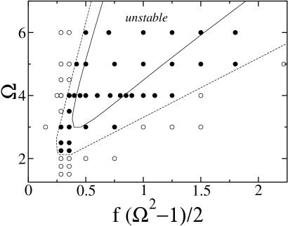
Figure 8: The $\Omega$-$f$ phase diagram for $\Lambda=81.09$. The solid curve is given by the granular hydrostatics: it shows the borders of the region where the annular state is unstable with respect to small perturbations. The filled symbols depict the parameters in which phase separated states are observed, whereas the hollow symbols show the parameters at which annular states are observed. The dashed line is an estimated binodal line of the system.

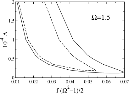
Figure 9: The marginal stability lines for our main setting (the solid line) and for an alternative setting in which the thermal wall is at $r=R_{\textit{ext}}$ and the elastic wall is at $r=R_{\textit{int}}$ (the dashed line).

IV Some modifications of the model

We also investigated an alternative setting in which the exterior wall is the driving wall, while the interior wall is elastic. The corresponding hydrostatic problem is determined by the same three scaled parameters $f$, $\Lambda$ and $\Omega$, but the boundary conditions must be changed accordingly. Here azimuthally symmetric clusters appear near the (elastic) interior wall. Symmetry breaking instability occurs here as well. We found very similar marginal stability curves here, but they are narrower (as shown in Fig. 9) than those obtained for the original setting.

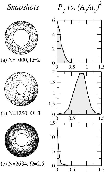
Figure 10: Typical steady state snapshots (the left column) and the normalized probability distribution functions $P_{1}\left(A_{1}^{2}/a_{0}^{2}\right)$ for an inelastic exterior wall, $\mu_{wall}=0.99$ (the right column) for different numbers of particles.

Finally, we returned to our original setting and performed several MD simulations, replacing the perfectly elastic exterior wall by a weakly inelastic one. The inelastic particle collisions with the exterior wall were modeled in the same way as the inelastic collisions between particles. Typical results of these simulations are shown in Fig. 10. It can be seen that, for the right choice of parameters, the phase separation persists. This result is important for a possible experimental test of our theory.

V Summary

We combined equations of granular hydrostatics and event-driven MD simulations to investigate spontaneous phase separation of a monodisperse gas of inelastically colliding hard disks in a two-dimensional annulus, the inner circle of which serves as a “thermal wall”. A marginal stability analysis yields a region of the parameter space where the annular state – the basic, azimuthally symmetric steady state of the system – is unstable with respect to small perturbations which break the azimuthal symmetry. The physics behind the instability is negative effective compressibility of the gas in the azimuthal direction, which results from the inelastic energy loss. MD simulations of this system show phase separation, but it is masked by large spatio-temporal fluctuations. By measuring the probability distribution of the amplitude of the fundamental Fourier mode of the azimuthal spectrum of the particle density we have been able to clearly identify the transition to phase separated states in the MD simulations. We have found that the instability region of the parameter space, predicted from hydrostatics, is located within the phase separation region observed in the MD simulations. This implies the presence of a binodal (coexistence) region, where the annular state is metastable, similar to what was found in rectangular geometry argentina ; khain2 . The instability persists in an alternative setting (a driving exterior wall and an elastic interior wall), and also when the elastic wall is replaced by a weakly inelastic one. We hope our results will stimulate experimental work on the phase separation instability.

VI Acknowledgments

This work grew out of a student research project at the 2003 Summer School “From pattern formation to granular physics and soft condensed matter” sponsored by the European Union under FP5 High Level Scientific Conferences, and by the NATO Advanced Study Institute. We are grateful to Igor Aranson, Pavel Sasorov and Thomas Schwager for advice. MDM acknowledges financial support from MEyC and FEDER (project FIS2005-00791). BM acknowledges financial support from the Israel Science Foundation (grant No. 107/05) and from the German-Israel Foundation for Scientific Research and Development (Grant I-795-166.10/2003).

References

- (1) H. R. Jaeger, S. Nagel, and R. P. Behringer, Rev. Mod. Phys. 68, 1259 (1996); Phys. Today 49(4), 32 (1996).
- (2) G.H. Ristow, Pattern Formation in Granular Materials (Springer Tracts in Modern Physics) (Springer, Berlin, 2000).
- (3) I.S. Aranson and L.S. Tsimring, Rev. Mod. Phys. 78, 641 (2006).
- (4) C. S. Campbell, Annu. Rev. Fluid Mech. 22, 57 (1990).
- (5) L. P. Kadanoff, Rev. Mod. Phys. 71, 435 (1999).
- (6) Granular Gases, edited by T. Pöschel and S. Luding (Springer, Berlin, 2001).
- (7) Granular Gas Dynamics, edited by T. Pöschel and N. Brilliantov (Springer, Berlin, 2001).
- (8) I. Goldhirsch, Annu. Rev. Fluid Mech. 35, 267 (2003).
- (9) N.V. Brilliantov N.V. and T. Pöschel, Kinetic Theory of Granular Gases, (Oxford University Press, Oxford, 2004).
- (10) N. Sela and I. Goldhirsch, J. Fluid Mech. 361, 41 (1998).
- (11) J. J. Brey, J. W. Dufty, C. S. Kim, and A. Santos, Phys. Rev. E 58, 4638 (1998).
- (12) J. F. Lutsko, Phys. Rev. E 72, 021306 (2005).
- (13) E. Livne, B. Meerson, and P. V. Sasorov, Phys. Rev. E 65, 021302 (2002); cond-mat/0008301 (2000).
- (14) M. Argentina, M.G. Clerc, and R. Soto, Phys. Rev. Lett. 89, 044301 (2002).
- (15) J. J. Brey, M. J. Ruiz-Montero, F. Moreno, and R. García-Rojo, Phys. Rev. E 65, 061302 (2002).
- (16) E. Khain and B. Meerson, Phys. Rev. E 66, 021306 (2002).
- (17) E. Livne, B. Meerson, and P.V. Sasorov, Phys. Rev. E 66, 050301(R) (2002).
- (18) B. Meerson, T. Pöschel, P. V. Sasorov, and T. Schwager, Phys. Rev. E 69, 021302 (2004).
- (19) E. Khain, B. Meerson, and P. V. Sasorov, Phys. Rev. E 70, 051310 (2004).
- (20) A. Kudrolli, M. Wolpert, and J. P. Gollub, Phys. Rev. Lett. 78, 1383 (1997).
- (21) Y. Du, H. Li, and L. P. Kadanoff, Phys. Rev. Lett. 74, 1268 (1995).
- (22) S. E. Esipov and T. Pöschel, J. Stat. Phys. 86, 1385 (1997).
- (23) E. L. Grossman, T. Zhou, and E. Ben-Naim, Phys. Rev. E 55, 4200 (1997).
- (24) J. T. Jenkins and M. W. Richman, Phys. Fluids 28, 3485 (1985).
- (25) N. F. Carnahan and K. E. Starling, J. Chem. Phys. 51, 635 (1969).
- (26) T. Pöschel and T. Schwager, Computational Granular Dynamics: Models and Algorithms. (Springer, Berlin, 2005).