Master singular behavior for the Sugden factor of the one-component fluids near their gas-liquid critical point

Abstract

We present the master (i.e. unique) behavior of the squared capillary length - so called the Sudgen factor-, as a function of the temperature-like field along the critical isochore, asymptotically close to the gas-liquid critical point of twenty (one component) fluids. This master behavior is obtained using the scale dilatation of the relevant physical fields of the one-component fluids. The scale dilatation introduces the fluid-dependent scale factors in a manner analog with the linear relations between physical fields and scaling fields needed by the renormalization theory applied to the Ising-like universality class. The master behavior for the Sudgen factor satisfies hyperscaling and can be asymptotically fitted by the leading terms of the theoretical crossover functions for the correlation length and the susceptibility in the homogeneous domain recently obtained from massive renormalization in field theory. In the absence of corresponding estimation of the theoretical crossover functions for the interfacial tension, we define the range of the temperature-like field where the master leading power law can be practically used to predict the singular behavior of the Sudgen factor in conformity with the theoretical description provided by the massive renormalization scheme within the extended asymptotic domain of the one-component fluid “subclass”.

I Introduction

The knowledge of interfacial properties Rowlinson 1984 for a nonhomogeneous fluid of coexisting vapor and liquid at equilibrium is of prime importance for many engineering applications and process simulations. Moreover, accurate predictions of these interfacial properties are essential to gain confidence in modeling underground geological fluid flows in porous media, oil recovery, gas storage in geological formations, pool boiling phenomena, microfluidic devices based on wetting phenomena, etc.

A large number of different forms of related phenomenological laws, the so-called ancillary equations, are reported in the literature to calculate interfacial properties along the vapor-liquid equilibrium (VLE) line Xiang 2005 . These relations complement the complex multiparameter equations of state (EOS’s) which have been developed to accurately fit the thermodynamic properties measured in the homogeneous domain. Such a phenomenological approach to estimate fluid properties is commonly based on the multiparameter corresponding-states principle Xiang 2005 ; Rowlinson 1971 ; Ely 2000 . In the following we call $n$-CSEOS such an EOS which contains $n\geq 2$ system-dependent parameters. The main reason for the power of such a phenomenological approach is related to the fact that the two-parameter corresponding-states ($2$-CS) principle can be applied to any polynomial EOS which has a liquid-vapor critical point Leach 1968 . However, in spite of increasing the number of fluid-dependent parameters, the common calculation of interfacial properties from ancillary equations and $n$-CSEOS, is not only mathematically complex, but is also unable to account for:

1) the molecular fluid complexity Rowlinson 1971 , especially the non-spherical symmetry of molecules and the quantum behavior of light fluids Ely 2000 ;

2) the asymptotic scaling of the critical phenomena close to the gas-liquid critical point Anisimov 2000 , especially the non-analytic Ising-like nature Privman 1991 ; ZinnJustin 2002 of the critical exponent Guida 1998 .

Among these interfacial properties, the capillary length $\ell_{Ca}$, or more precisely the squared capillary length $\left(\ell_{Ca}\right)^{2}$ also called the Sugden factor Sudgen 1924 and noted $S_{g}$ in the following, plays a special role on Earth’s gravity environment (recalled here by the subscript $g$). The Sugden factor reflects the balance between interfacial and volumic forces which defines the shape and the position of the interface in equilibrium when subject to the gravity field of constant acceleration $g$. In the case of perfect liquid wetting,$S_{g}$ is then related to the surface tension $\sigma$ and the density difference $\Delta\rho_{LV}=\rho_{L}-\rho_{V}$ between coexisting liquid (density $\rho_{L}$) and vapor (density $\rho_{V}$) phases by the equation

$$S_{g}=\frac{2\sigma}{g\Delta\rho_{LV}}$$ (1)

where $\sigma$ is the surface tension. Therefore, the knowledge of the Sugden factor is an important challenge to provide better control on non homogeneous fluid properties.

In addition, as clearly documented two decades ago Rathjen 1977 sulfurhexafluoride-halocarbons ; Gielen 1984 Ar-N2-O2-CO2-CH4 ; Moldover 1985 , the temperature dependence of $S_{g}$, along a large temperature range of the VLE line of all investigated one-component fluids Maass 1921 Ethane-Ethylene ; Coffin 1928 i-butane ; Katz 1939 2-3alcane ; Stansfield 1958 Argon-Nitrogen ; Smith 1967 Xenon ; Grigull 1969 Carbondioxide ; Gielen 1984 Ar-N2-O2-CO2-CH4 ; Rathjen 1977 sulfurhexafluoride-halocarbons ; Straub 1980 water ; Vargaftik 1983 Water ; Rathjen 1980 , shows a pure power law behavior which is applicable over an appreciably larger temperature range [see below Eq. (2) and the related dicussion of the Fig. 1a]. Such a weak temperature dependence of the effective exponent at small but finite distance of the critical point was partly well-understood to be related to the smallest value ($\simeq 0.51$ Guida 1998 , see below) of the confluent exponents which govern the corrections to asymptotic scaling of critical phenemonena Wegner 1972 . However the theoretical reason to observe a near zero-value of the amplitude contribution of the confluent corrections for the Sugden factor case remains unclear, specially in the absence of estimation of the crossover behavior of the surface tension.

Indeed, the significant theoretical improvements to account for classical-to-critical crossover ZinnJustin 2002 , specially in the one-component fluids Anisimov 2000 , provide the most powerful tools available today to analyze accurately interfacial properties in large temperature ranges of the non-homogeneous domain. For example in the present work, using the crossover functions recently derived Bagnuls 2002 ; Garrabos 2006c from the massive renormalization scheme Bagnuls 1984a ; Bagnuls 1984b ; Bagnuls 1985 ; Bagnuls 1987 , our main objective is to accurately estimate this leading asymptotic behavior of $S_{g}$ from scaling arguements Widom 1965 ; Fisk 1969 ; Stauffer 1972 ; Rowlinson 1984 and available MR description Garrabos 2006a ; Garrabos 2006d ; Garrabos 2006e of the master singular behavior of the one-component fluid “subclass”. Such a description is based on the formal analogy between the scale dilatation of the physical field variables proposed by Garrabos Garrabos 1982 ; Garrabos 1985 ; Garrabos 2006b and the linear relation between the physical fields and the scaling fields needed by the renormalization theory Wilson 1971 . The major advantage of this scale dilatation method is to estimate the universal behavior of any one-component fluids without adjustable parameters, by using only the four critical coordinates of its liquid-vapor critical point (excluding here quantum fluids Garrabos 2006b to simplify the presentation of the scale dilatation method).

The paper is organized as follows. Section 2 demonstrates the master singular behavior of $S_{g}$ observed from the scale dilatation method. The corresponding Ising-like asymptotic description of $S_{g}$ based on hyperscaling Widom 1965 ; Fisk 1969 ; Stauffer 1972 ; Rowlinson 1984 and MR description Bagnuls 1984a ; Bagnuls 1985 ; Bagnuls 1987 of the critical crossover is reported in Section 3. The master leading terms of the MR crossover functions for the correlation length and the susceptibility in the homogeneous domain Bagnuls 2002 ; Garrabos 2006c , are used to demonstrate that the fit of the master behavior observed in the (nonhomogeneous) extended asymptotic domain can be made with a theoretical precision of the same order of magnitude than the experimental one. The discussion given in Section 4 shows the main points to be considered for a classical-to-critical crossover description of the interfacial properties at finite temperature distance to the critical temperature. Specifically, we estimate precisely the temperature-like range where this theoretical treatment becomes unappropriate to represent the increasing non critical microscopic difference between gas and liquid approaching the triple point temperature. Conclusion is given in Section 5.

II Master singular behavior of the Sugden factor

II.1 The data sources

The Sugden factor measurements $S_{g}\left(\left|\Delta T\right|\right)$ as a function of the temperature distance $\Delta T=T-T_{c}$ to the critical point in the nonhomogeneous range $T<T_{c}$, have been published and analyzed for several one-component fluids Maass 1921 Ethane-Ethylene ; Coffin 1928 i-butane ; Katz 1939 2-3alcane ; Stansfield 1958 Argon-Nitrogen ; Smith 1967 Xenon ; Grigull 1969 Carbondioxide ; Gielen 1984 Ar-N2-O2-CO2-CH4 ; Rathjen 1977 sulfurhexafluoride-halocarbons ; Straub 1980 water ; Vargaftik 1983 Water ; Rathjen 1980 ; Moldover 1985 ; Grigoryev 1992 5-8alcane . $T$ ($T_{c}$) is the temperature (critical temperature). $S_{g}\left(\left|\Delta T\right|\right)$ data are generally obtained along the critical isochore $\rho=\rho_{c}$ in a finite temperature range bounded by max and min values of $\left|\Delta T\right|=T_{c,exp}-T$, where $T_{c,exp}$ is the measured (or estimated) critical temperature in the experiments [$\rho$ ($\rho_{c}$) is the density (critical density)]. The relative precision clamed by the authors is generally lower than $10\%$. For most fluids, $S_{g}$ was fitted using the effective power law of equation Rowlinson 1984 ; Rathjen 1977 sulfurhexafluoride-halocarbons ; Moldover 1985

$$S_{g}=S_{0,e}\left|\Delta\tau^{*}\right|^{\varphi_{e}}$$ (2)

where the dimensionless temperature distance $\left|\Delta\tau^{\ast}\right|$ to the critical point was defined by

$$\left|\Delta\tau^{\ast}\right|=\frac{\left|\Delta T\right|}{T_{c,exp}}=\frac{T_{c,exp}-T}{T_{c,exp}}$$ (3)

In Eq. (2), the free amplitude $S_{0,e}$ was a fluid-dependent quantity related to the effective value $\varphi_{e}\simeq 0.91-0.97$ of the free (or fixed) exponent $\varphi_{e}$ considered as an adjustable parameter when measurements were performed in a restricted temperature range at finite distance to $T_{c,exp}$. The corresponding results $\varphi_{e}$;$S_{0,e}$ [with free (or fixed) value of $\varphi_{e}$] for each selected fluid are summarized in columns 3 and 4 of Table 1 (references are given in column 2). However, admitting now that $\Delta\tau^{\ast}$ is the relevant physical field Widom 1965 to describe the singular scaling behavior of the thermodynamic fluid properties in the homogeneous or nonhomogenous domains along the critical isochore, the three main “critical phenomena” features of these fitting analyses are:

i) the correlation between the effective values of $S_{0,e}$ and $\varphi_{e}$ is highly dependent on $T_{c,exp}$ and on the (min and max) values of the temperature range covered by the fit “close” to the critical point; especially when the local values of $\varphi_{e}$ are estimated in the temperature range lower than $\left|\Delta\tau^{\ast}\right|<0.05$, the common averaged value $\varphi_{e}=0.935\pm 0.015$, equal to the asymptotic universal value $\varphi=2\nu-\beta=0.935\pm 0.015$ obtained from the present theoretical estimation of the critical exponents $\nu=$ and $\beta=$ Guida 1998 [see below Eq. (5)], appears consistent with the $S_{g}$ data, whatever the one-component fluid.

ii) accordingly, the temperature dependence of the effective exponent over a larger temperature range is very small (then with a sign not unambiguously defined for the small amplitude of the leading confluent term), whatever the one-component fluid or the extension of the temperature range of the fit;

iii) the measured value of the effective exponent is never equal to the mean-field value $\varphi_{MF}=1$, whatever the one-component fluid and even the large temperature range of the fit;

As a matter of fact, it is well-established now ZinnJustin 2002 that the range of validity of the asymptotic scaling form of Eq. (2) is, strictly restricted to the asymptotic approach of the liquid-gas critical point (CP), when $\sigma\propto\left|\Delta\tau^{*}\right|^{\phi}$ and $\Delta\rho_{LV}\propto\left|\Delta\tau^{*}\right|^{\beta}$ simultaneously go to zero for $\Delta\tau^{\ast}\rightarrow 0$ in Eq. (1). $\phi=\left(d-1\right)\nu\approx 1.261$ and $\beta\approx 0.326$ are the universal values Guida 1998 of the critical exponents related to $\sigma$ and $\Delta\rho_{LV}$, respectively, and $\nu\approx 0.63$ is the universal value Guida 1998 of the critical exponent for the correlation length, with $\xi\propto\left|\Delta\tau^{*}\right|^{-\nu}$ (see also ZinnJustin 2002 for details of notations and definitions). However, at small but finite $\left|\Delta\tau^{*}\right|$, any pure power law like Eq. (2) must be modified to account for confluent corrections to scaling which can be represented by the Wegner-like expansion Wegner 1972 with the universal features of uniaxial 3D Ising like systems ZinnJustin 2002 . Then, the asymptotic singular decrease of $S_{g}$ must be fitted by the following equation

$$S_{g}=S_{0}\left|\Delta\tau^{*}\right|^{\varphi}\left[1+{\displaystyle\sum_{i=1}^{\infty}}S_{i}\left|\Delta\tau^{*}\right|^{i\Delta}\right]$$ (4)

where $\Delta\approx 0.51$ is the universal value Guida 1998 of the critical exponent which characterizes the leading family of the confluent corrections to scaling. The amplitudes $S_{0}$, $S_{1}$, … $S_{i}$, etc., are fluid-dependent quantities. Equation (4) means that the critical exponent

$$\varphi=\phi-\beta=\left(d-1\right)\nu-\beta$$ (5)

only takes its universal value $\varphi\approx 0.935$ asymptotically when $\Delta\tau^{\ast}\rightarrow 0$. Therefore, the weak temperature dependence of the effective exponent at finite value of $\Delta\tau^{*}$, first shows low rate of convergence of the Wegner expansion. Moreover, in the fitting of the experimental $S_{g}$ data, if the contribution of the confluent correction terms is negligible, then ${\displaystyle\sum_{i=1}^{\infty}}S_{i}\left|\Delta\tau^{*}\right|^{i\Delta}\sim 0$ in Eq. (4).

Fluid	Ref	$\varphi_{e}$	$S_{0,e}$	$S_{0,\varphi}$	Ref	$\mathcal{Z}_{S,\varphi}$	$\delta\mathcal{Z}_{S,\varphi}$
			$\left(mm^{2}\right)$	$\left(mm^{2}\right)$			$\%$
$Ar$	Stansfield 1958 Argon-Nitrogen	$0.940$	$4.13$	$4.036$	Moldover 1985	$2.423$	$-1.9$
	Gielen 1984 Ar-N2-O2-CO2-CH4	$0.913$	$3.78$	$4.18$	This work	$2.510$	$+1.6$
$Xe$	Smith 1967 Xenon	$0.942$	$3.05$	$2.953$	Moldover 1985	$2.668$	$+8.0$
$N_{2}$	Stansfield 1958 Argon-Nitrogen	$0.930$	$5.46$	$5.59$	This work	$2.446$	$-1.0$
	Gielen 1984 Ar-N2-O2-CO2-CH4	$0.926$	$5.10$	$5.32$	This work	$2.328$	$-5.7$
$O_{2}$	Gielen 1984 Ar-N2-O2-CO2-CH4	$0.909$	$4.85$	$5.47$	This work	$2.563$	$+4.6$
$CO_{2}$	Grigull 1969 Carbondioxide	$0.933$	$9.47$	$9.52$	Moldover 1985	$2.55$	$+3.3$
	Gielen 1984 Ar-N2-O2-CO2-CH4	$0.920$	$8.40$	$9.0$	This work	$2.411$	$-2.4$
$SF_{6}$	Rathjen 1977 sulfurhexafluoride-halocarbons	$0.943$	$3.931$	$3.84$	Moldover 1985	$2.46$	$-0.4$
$CCl_{3}F$	Rathjen 1977 sulfurhexafluoride-halocarbons	$0.928$	$6.234$	$6.44$	This work	$2.470$	$0.0$
$CCl_{2}F_{2}$	Rathjen 1977 sulfurhexafluoride-halocarbons	$0.936$	$5.615$	$5.589$	This work	$2.476$	$+0.3$
$CClF_{3}$	Grigull 1969 Carbondioxide	$0.972$	$5.33$	$4.5$	This work	$2.268$	$-8.1$
	Rathjen 1977 sulfurhexafluoride-halocarbons	$0.9379$	$4.847$	$4.783$	This work	$2.411$	$-2.4$
$CBrF_{3}$	Rathjen 1977 sulfurhexafluoride-halocarbons	$0.938$	$3.879$	$3.826$	This work	$2.374$	$-3.1$
$CHClF_{2}$	Rathjen 1977 sulfurhexafluoride-halocarbons	$0.937$	$6.859$	$6.796$	This work	$2.323$	$-6.0$
$C_{2}H_{4}$	Maass 1921 Ethane-Ethylene			$13.90$	Moldover 1985	$2.480$	$+0.4$
$CH_{4}$	Gielen 1984 Ar-N2-O2-CO2-CH4	$0.933$	$13.6$	$13.73$	This work	$2.382$	$-3.6$
$C_{2}H_{6}$	Maass 1921 Ethane-Ethylene ; Katz 1939 2-3alcane			$14.42$	Moldover 1985	$2.437$	$-1.3$
$i-C_{4}H_{10}$	Coffin 1928 i-butane			$12.71$	Moldover 1985	$2.392$	$-3.2$
$n-C_{5}H_{12}$	Grigoryev 1992 5-8alcane	$0.935$	$12.916$			$2.488$	$+0.7$
$n-C_{6}H_{14}$	Grigoryev 1992 5-8alcane	$0.935$	$12.753$			$2.445$	$-1.0$
$n-C_{7}H_{16}$	Grigoryev 1992 5-8alcane	$0.935$	$12.520$			$2.552$	$+3.4$
$n-C_{8}H_{18}$	Grigoryev 1992 5-8alcane	$0.935$	$12.217$			$2.520$	$+2.0$
$H_{2}O$	Vargaftik 1983 Water			$34.72$	Moldover 1985	$2.262$	$-8.4$
	Straub 1980 water	$0.91$	$33.2$	$37.25$	This work	$2.427$	$-1.7$
$\left\langle\mathcal{Z}_{S,\varphi}\right\rangle$						$2.4530$	$\pm 3.1$
$\mathcal{Z}_{S}$						$2.47$

Table 1: Effective leading amplitude $S_{0,e}$ [see Eq. (2)] of the Sugden factor $S_{g}\equiv\left(\ell_{Ca}\right)^{2}$ ($\ell_{Ca}$ is the capillary length) (column 2) for several one-component fluids (colum 1); Calculated values of the master amplitude$\mathcal{Z}_{S,e}$ (column 3) of the renormalized Sugden factor $\mathcal{S}_{g^{*}}^{*}$ [see Eq. (18)], using Eq. (22); The residual $\delta\mathcal{Z}_{S}=100\times\left(\frac{\left(\mathcal{Z}_{S}\right)_{exp}}{\mathcal{Z}_{S}}-1\right)$ (expressed in %) from the value $\mathcal{Z}_{S}=2.47$ estimated from Eq. (43) is given in column 4; (for data sources and the selected fitting results see the references given in the last column).

To illustrate this behavior, the Sugden factor $S_{g}\equiv\left(\ell_{Ca}\right)^{2}$ (expressed in $m^{2}$) can be divided by $\left(T_{c}-T\right)^{\varphi}$ (expressed in $K^{\varphi}$, with $\varphi=0.935$) Moldover 1985 . In Figure 1a (log-log scale), this convenient scaled form $\frac{S_{g}}{\left(T_{c}-T\right)^{\varphi}}$ [$m^{2}\,K^{-\varphi}$], is shown as a function of the temperature distance $T_{c}-T$ [$K$] for eighteen one-component fluids. Each curve has a relative temperature extension corresponding to the experimental temperature range (including for some fluids measurements until their triple point temperature $T_{TP}$). The use of such dimensional quantities makes the order of magnitude of the leading amplitude contribution (i.e. $S_{g}\left(T=T_{c}+1K\right)\simeq S_{0}\left(T_{c}\right)^{-\varphi}$) of each fluid clearly distinguishable, while the quasi-horizontal line whatever the fluid (except the water case which needs a special attention given in § 4.3) shows that the confluent contribution is negligible (i.e. ${\displaystyle\sum_{i=1}^{\infty}}S_{i}\left(T_{c}\right)^{-i\Delta}\left(T_{c}-T\right)^{i\Delta}\sim 0$). $S_{g}$ values at $T_{c}-T=1\,K$ cover one decade: from $1.5\,10^{-8}\,m^{2}$ for sulfurhexafluoride [with $S_{0}\left(SF_{6}\right)=3.84\,mm^{2}$], to $1.5\,10^{-7}\,m^{2}$ for methane [$S_{0}\left(CH_{4}\right)=13.80\,mm^{2}$].

We have noted that some of the data reported in Fig. 1a have been measured in a large temperature range of the coexisting VLE line, including measurements close to $T_{TP}$. To separate the asymptotic critical range from the triple point location along the temperature axis, we have marked by vertical arrows the temperature distance where $T=0.7\,T_{c}$ (i.e. the temperature distance where the practical fluid-dependent acentric factor Pitzer1955 is defined in the nonhomogeneous domain). The “non-critical” temperature range between $0.3\,T_{c}\leq T_{c}-T\leq T_{c}-T_{TP}$ (the right hand side of the corresponding arrows in Fig. 1a) is considered to be far away from the critical point. Close to the critical point, the practical temperature range where the Wegner-like expansion fit the singular behavior does not usually exceed a few percent in $\left|\Delta\tau^{*}\right|$ Levelt-Sengers 1981 . In a similar arbitrary manner, we have represented by vertical arrows the temperature distance where $T=0.99\,T_{c}$, to make clear the “critical” temperature range $T_{c}-T\leq 0.01\,T_{c}$ (the left hand side of the corresponding arrows in Fig. 1a), where the use of Eq. (4) has a theoretical justification, as discussed below in § 3. To introduce the main physical parameters needed for accurate description of the singular behavior of $S_{g}$ in this asymptotic temperature range, the next subsection presents the application of the scale dilatation method Garrabos 1982 ; Garrabos 1985 leading to define the dimensionless form (noted $S_{g}^{*}$) and the renormalized form (noted $\mathcal{S}_{g^{*}}^{*}$) of the Sugden factor, with two objectives:

1) to show that any modeling based on the $2$-CS principle is inaccurate to describe the fluid dependence of (dimensionless) $S_{g}^{*}$ [see below Eq. (12)] as a function of the (dimensionless) temperature field $\Delta\tau^{*}$;

2) to unambiguously show the master singular behavior of (renormalized) $\mathcal{S}_{g^{*}}^{*}$ [see below Eq. (18)] as a function of the (renormalized) temperature-like field, noted $\mathcal{T}^{*}$ [see below Eq. (14)] .

II.2 The scale dilatation method to observe the master singular behavior

The following analysis of the Sugden factor from the scale dilatation method is similar to the one of the correlation length given in Ref. Garrabos 2006a . We recall only the main features (ignoring the quantum contributions at $T\cong T_{c}$ Garrabos 2006b ). The input data are the four critical coordinates

$$Q_{c,a_{\bar{p}}}^{min}=\left\{T_{c},v_{\bar{p},c},p_{c},\gamma_{c}^{\prime}=\left[\left(\frac{\partial p}{\partial T}\right)_{v_{\bar{p},c}}\right]_{CP}\right\}$$ (6)

which localize the liquid gas critical point on the phase surface of equation $\Phi_{a_{\bar{p}}}^{p}\left(p,v_{\bar{p}},T\right)=0$ for each fluid particle of mass $m_{\bar{p}}$ particle mass . $p$ is the pressure, $v_{\bar{p}}$ is the particle volume, and $a_{\bar{p}}\left(T,v_{\bar{p}}\right)$ is the Helmholtz energy per particle. The subscript $\bar{p}$ refers to a particle quantity and all the definitions and notations related to Eq. (6) are given in Garrabos 1982 ; Garrabos 1985 ; Garrabos 2006b . The critical data related to the fluids selected in Table 1 are reported in Table 2. We note that $T_{c}$ values of Table 2, which were obtained from the thermodynamic analysis of the phase surface, can be slightly different from $T_{c,exp}$ values given in the experiments refered in Table 1. Also $\rho_{c}=\frac{m_{\bar{p}}}{v_{\bar{p},c}}$ values from Table 2 can be slightly different from the experimental critical density values reported in these experiments.

Fluid	$\begin{array}[]{c}m_{\bar{p}}\\ \left(10^{-26}kg\right)\end{array}$	$\begin{array}[]{c}T_{c}\\ \left(K\right)\end{array}$	$\begin{array}[]{c}v_{\bar{p},c}\\ \left(nm^{3}\right)\end{array}$	$\begin{array}[]{c}p_{c}\\ \left(MPa\right)\end{array}$	$\begin{array}[]{c}\gamma_{c}^{\prime}\\ \left(MPa\,K^{-1}\right)\end{array}$	$\begin{array}[]{c}\left(\beta_{c}\right)^{-1}\\ \left(10^{-21}J\right)\end{array}$	$\begin{array}[]{c}\alpha_{c}\\ \left(nm\right)\end{array}$	$Z_{c}$	$Y_{c}$
$Ar$	$6.634$	$150.725$	$0.12388$	$4.865$	$0.191$	$2.08099$	$0.753463$	$0.2896$	$4.32882$
$Xe$	$21.803$	$289.733$	$0.19589$	$5.84$	$0.1182$	$4.0003$	$0.881508$	$0.28601$	$4.85434$
$N_{2}$	$4.652$	$126.214$	$0.14814$	$3.398$	$0.1715$	$1.74258$	$0.80043$	$0.288875$	$5.37014$
$O_{2}$	$5.314$	$154.580$	$0.12187$	$5.043$	$0.1953$	$2.13421$	$0.750786$	$0.287972$	$4.98641$
$CO_{2}$	$7.308$	$304.137$	$0.15622$	$7.3753$	$0.170$	$4.19907$	$0.82882$	$0.27438$	$6.0104$
$SF_{6}$	$24.255$	$318.735$	$0.32769$	$3.754$	$0.0835$	$4.40062$	$1.0544$	$0.27954$	$6.0896$
$CCl_{3}F$	$22.810$	$471.110$	$0.41174$	$4.4076$	$0.0655$	$6.50438$	$1.13850$	$0.27901$	$6.00530$
$CCl_{2}F_{2}$	$20.078$	$384.930$	$0.35562$	$4.1249$	$0.0745$	$5.31454$	$1.08814$	$0.27602$	$5.95186$
$CClF_{3}$	$17.348$	$301.88$	$0.29807$	$3.877$	$0.0910$	$4.16791$	$1.02441$	$0.27727$	$6.08861$
$CBrF_{3}$	$24.727$	$340.19$	$0.33191$	$3.956$	$0.0810$	$4.69683$	$1.05889$	$0.27956$	$5.96985$
$CHClF_{2}$	$14.359$	$369.30$	$0.27454$	$4.990$	$0.0965$	$5.09874$	$1.00721$	$0.26869$	$6.14259$
$C_{2}H_{4}$	$4.658$	$282.345$	$0.21667$	$5.042$	$0.11337$	$3.89820$	$0.91781$	$0.28131$	$5.34856$
$CH_{4}$	$2.664$	$190.564$	$0.16361$	$4.5992$	$0.14442$	$2.63102$	$0.830133$	$0.28679$	$4.9838$
$C_{2}H_{6}$	$4.993$	$305.322$	$0.24171$	$4.872$	$0.10304$	$4.21554$	$0.95290$	$0.27935$	$5.45505$
$i-C_{4}H_{10}$	$9.652$	$407.844$	0.43020	$3.629$	$0.0610$	$5.63084$	$1.15770$	$0.27726$	$5.93407$
$n-C_{5}H_{12}$	$11.981$	$469.70$	$0.521785$	$3.3665$	$0.0511$	$6.48491$	$1.24425$	$0.270875$	$6.12956$
$n-C_{6}H_{14}$	$14.310$	$507.49$	$0.61138$	$3.0181$	$0.043658*$	$7.00666$	$1.3186$	$0.26667$	$6.30719$
$n-C_{7}H_{16}$	$16.6386$	$540.13$	$0.7168$	$2.727$	$0.038068*$	$7.45731$	$1.3983$	$0.26218$	$6.64356$
$n-C_{8}H_{18}$	$18.9683$	$568.88$	$0.81839$	$2.486$	$0.033768*$	$7.85424$	$1.46746$	$0.258978$	$6.82776$
$H_{2}O$	$2.991$	$647.067$	$0.09268$	$22.046$	$0.275$	$8.93373$	$0.740$	$0.229$	$7.071$

Table 2: Set of critical parameters [see Eqs. (6) and (7)] for twenty one-component fluids of particle mass $m_{\bar{p}}$ particle mass selected in the present work (see Fig. 1).

In combining $Q_{c,a_{\bar{p}}}^{\min}$, the Boltzmann constant $k_{B}$, and $d=3$, Eq. (6) can be written in a more convenient form, such that

$$Q_{c}^{\min}=\left\{\left(\beta_{c}\right)^{-1},\alpha_{c},Z_{c},Y_{c}\right\}$$ (7)

which introduces the following four scale factors given by,

$$\left(\beta_{c}\right)^{-1}=k_{B}T_{c}$$ (8)

$$\alpha_{c}=\left(\frac{k_{B}T_{c}}{p_{c}}\right)^{\frac{1}{d}}$$ (9)

$$Z_{c}=\frac{p_{c}v_{\bar{p},c}}{k_{B}T_{c}}$$ (10)

$$Y_{c}=\gamma_{c}^{\prime}\frac{T_{c}}{p_{c}}-1$$ (11)

Equation (7) involves one energy scale unit $\left(\beta_{c}\right)^{-1}$, one length scale unit $\alpha_{c}$, and two dimensionless scale factors $Z_{c}$ and $Y_{c}$ characterizing two preferred directions to cross the critical point along the critical isotherm and the critical isochore, respectively. $\alpha_{c}$, which does not depend of the size $L\sim\left(V\right)^{\frac{1}{d}}$ of the container, has a clear physical meaning as length unit Garrabos 1982 : it represents the spatial extent of the short-ranged (Lennard-Jones like) molecular interaction Hirschfelder 1964 , which allows us to define $v_{c,I}=\frac{k_{B}T_{c}}{p_{c}}$ as the volume of the microscopic critical interaction cell (CIC) of each fluid. $Z_{c}$ is the usual critical compression factor. Furthermore, $\left(Z_{c}\right)^{-1}=n_{c}v_{c,I}$ is the number of particles that fills $v_{c,I}$. Then the minimal set of data in Eq. (7) is related to the thermodynamic properties of the critical interaction cell of size $\alpha_{c}=\left(v_{c,I}\right)^{\frac{1}{d}}$ Garrabos 2005 .

We recall that the critical compression factor $Z_{c}$, and the critical Riedel factor $\alpha_{R,c}$ Riedel 1954 [related to $Y_{c}$ by $\alpha_{R,c}=Y_{c}+1$], are among the basic parameters used to develop $4$-CSEOS’s for engineering fluid modeling Poling 2001 .

The characteristic units $\left(\beta_{c}\right)^{-1}$ and $\alpha_{c}$ are the parameters needed to provide a dimensionless analysis of the fluid properties, leading to their “classical” description based on the two-parameter corresponding state ($2$-CS) description. Obviously, the dimensionless form of the Sugden factor is given by

$$S_{g}^{*}=\frac{S_{g}}{\left(\alpha_{c}\right)^{2}}$$ (12)

Figure 1b (log-log scale; color online) represents the confluent behavior of the rescaled dimensionless quantity $\frac{S_{g}^{*}}{\left|\Delta\tau^{*}\right|^{\varphi}}$ as a function of the dimensionless temperature distance $\Delta\tau^{\ast}$. Figure 1b complements Fig. 3 initially published by Moldover in Ref. Moldover 1985 , after normalization of the vertical axis by $\left(\alpha_{c}\right)^{2}$. Figure 1b illustrates the results of any classical two-parameter corresponding state theory (here the two characteristic parameters are $\left(\beta_{c}\right)^{-1}$ and $\alpha_{c}$). Figure 1b, shows the failure of the $2$-CS principle in terms of molecular fluid complexity since, from xenon to water, the dimensionless Sugden factor covers one order of magnitude at the same reduced temperature distance to the critical point. Moreover, in terms of classical critical phenomena, using Eq. (1) where $\Delta\rho_{LV}\propto\left|\Delta\tau^{*}\right|^{\beta_{MF}}$ and $\sigma\propto\left|\Delta\tau^{*}\right|^{\phi_{MF}}$ with $\beta_{MF}=\frac{1}{2}$ and $\phi_{MF}=\frac{3}{2}$ Widom 1996 , we obtain the mean field exponent $\varphi_{MF}=1$. This mean-field value associated to the classical behavior of the correlation length (with exponent $\nu_{MF}=\frac{1}{2}$) expected from Van der Waals-like theories Widom 1996 ; Kostrowicka 2004 , is unable to describe the experimental results, even at large temperature distance, as shown by the significantly positive slope $\varphi_{MF}-\varphi\simeq 0.065$ reported in Fig. 1b. In addition, the scaling law $\left(d-1\right)\nu=\phi$, that explicitly involve $d$, is not correct for mean-field exponents in three dimension. We will turn back on the mean-field theories in § 4.2 when we will discuss the related critical-to-critical crossover description of the interfacial properties.

In the next step, the dimensionless scale factors $Y_{c}$ and $Z_{c}$ are introduced throughout the scale dilatation method Garrabos 1985 . Typically, the scale dilatation of the dimensionless temperature distance,

$$\Delta\tau^{\ast}=k_{B}\beta_{c}\left(T-T_{c}\right)$$ (13)

leads to the renormalized thermal field,

$$\mathcal{T}^{\ast}=Y_{c}\Delta\tau^{*}$$ (14)

The scale dilatation of the dimensionless order parameter density

$$\Delta m^{*}=\left(\alpha_{c}\right)^{d}\left(n-n_{c}\right)=\left(Z_{c}\right)^{-1}\Delta\tilde{\rho}$$ (15)

leads to the renormalized order parameter density

$$\mathcal{M}^{*}=\left(Z_{c}\right)^{\frac{d}{2}}\Delta m^{*}=\left(Z_{c}\right)^{\frac{1}{2}}\Delta\tilde{\rho}$$ (16)

In addition, the renormalized form $\ell^{*}\equiv\xi^{*}=\frac{\xi}{\alpha_{c}}$ of the correlation length $\xi$ Garrabos 2006b , leads to the renormalized form, noted $\Sigma^{*}$, of the surface tension $\sigma$ such that LeNeindre 2002

$$\Sigma^{*}\equiv\sigma^{*}=\sigma\beta_{c}\left(\alpha_{c}\right)^{d-1}$$ (17)

Taking into account Eqs. (1) and (12), the renormalized Sugden factor $\mathcal{S}_{g^{*}}^{*}$ reads as follows LeNeindre 2002

$$\mathcal{S}_{g^{*}}^{*}=g^{*}\left(Z_{c}\right)^{-\frac{3}{2}}\left(\ell_{Ca}^{*}\right)^{d-1}=g^{*}\left(Z_{c}\right)^{-\frac{3}{2}}S_{g}^{*}$$ (18)

with $g^{*}=m_{\bar{p}}\beta_{c}\alpha_{c}g$. Therefore, after application of the scale dilatation method, the renormalized form of Eq. (1) is given by

$$\mathcal{S}_{g^{*}}^{*}=\frac{\Sigma^{*}}{\mathcal{M}_{LV}^{*}}$$ (19)

As expected Garrabos 1982 , the collapse on the master curve obtained from the scale transformations

$$\begin{array}[]{cl}\Delta\tau^{*}&\rightarrow\mathcal{T}^{\ast}=Y_{c}\Delta\tau^{*}\\ S_{g}^{*}&\rightarrow\mathcal{S}_{g^{*}}^{*}=g^{*}\left(Z_{c}\right)^{-\frac{3}{2}}S_{g}^{*}\;\;\left(T1\,case\right)\\ &\rightarrow\mathcal{S}_{g^{*}}^{*}\times\left|\mathcal{T}^{\ast}\right|^{-\varphi}\;\;\;\;\;\;\;\;\;\;\;\left(T2\,case\right)\end{array}$$ (20)

is shown in Fig. 1c ($T1\,case$) and 1d ($T2\,case$), independently of any theoretical form used to represent this master behavior. Now the scatter of the collapsed data corresponds to the estimated precision ($10\%$) for the Sugden factor of each fluid.

II.3 Predictive power of the scale dilatation method within the Ising-like preasymptotic domain

As initially shown in Ref. Garrabos 1985 , we can expect to fit the master singular behavior of $\mathcal{S}_{g^{*}}^{*}$ observed asymptotically close to the critical temperature by a restricted (two-term) Wegner-like expansion given by

$$\mathcal{S}_{g^{*}}^{*}=\mathcal{Z}_{\mathcal{S}}\left|\mathcal{T}^{*}\right|^{\phi}\left[1+\mathcal{Z}_{\mathcal{S}}^{1}\left|\mathcal{T}^{*}\right|^{\Delta}\right]$$ (21)

where $\phi\approx 0.935$ and $\Delta\approx 0.51$ are the universal critical exponents while $\mathcal{Z}_{\mathcal{S}}$ and $\mathcal{Z}_{\mathcal{S}}^{1}$ are the master (i.e. unique) leading and confluent amplitudes, respectively, for all one-components fluids. By term to term comparison of Eqs. (4) and (21) using Eqs. (20), we obtain the following relations

$$\mathcal{Z}_{\mathcal{S}}=g^{*}\left(\alpha_{c}\right)^{1-d}\left(Z_{c}\right)^{-\frac{3}{2}}\left(Y_{c}\right)^{-\varphi}S_{0}$$ (22)

$$\mathcal{Z}_{\mathcal{S}}^{1}=\left(Y_{c}\right)^{-\Delta}S_{1}$$ (23)

which shows the unequivocal link between master amplitudes and system-dependent amplitudes, through $Q_{c}^{\min}$ [(Eq. (7)].

In other words, only when the fluid-dependent set $Q_{c}^{\min}$ and the master amplitudes $\mathcal{Z}_{\mathcal{S}}$ and $\mathcal{Z}_{\mathcal{S}}^{1}$ are known, the restricted Wegner-like expansion [Eq. (4) with $i\leq 1$] of $S_{g}$ can be determined for any one-component fluid by inverting Eqs.(22) and (23), such that $S_{0}=\left(\alpha_{c}\right)^{d-1}\left(g^{*}\right)^{-1}\left(Z_{c}\right)^{\frac{3}{2}}\left(Y_{c}\right)^{\varphi}\mathcal{Z}_{\mathcal{S}}$ and $S_{1}=\left(Y_{c}\right)^{\Delta}\mathcal{Z}_{\mathcal{S}}^{1}$. Then, the master values of $\mathcal{Z}_{\mathcal{S}}$ and $\mathcal{Z}_{\mathcal{S}}^{1}$ conform to the universal features calculated for the Ising-like universality class (i.e., some combinations and ratios of $\mathcal{Z}_{\mathcal{S}}$ and $\mathcal{Z}_{\mathcal{S}}^{1}$ take universal values, in agreement with the two-scale-factor universality). We will detail this point in § 4. Before, in the next Section, the scale transformations of Eq. (20) are reported in conformity with the asymptotic linearization Wilson 1971 of the two relevant fields needed by the renormalization group theory. That leads indeed to the correct account for universal features estimated in the preasymptotic domain and the accurate determination of $\mathcal{Z}_{\mathcal{S}}$ using the present theoretical status provided by the MR scheme Guida 1998 ; Bagnuls 2002 .

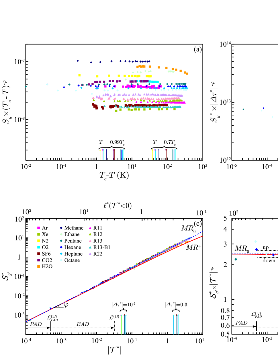
Figure 1: (Color online) a) Singular behavior (log-log scale) of $\frac{S_{g}}{\left(T_{c}-T\right)^{\varphi}}$ (expressed in $m^{2}\,K^{-\varphi}$, with $\varphi=0.935$), as a function of the temperature distance $T_{c}-T$, for nonhomogeneous one-component fluids (see Tables I and II). For each fluid, the arrows indicate the arbitrary temperature distances of $T_{c}-T=0.01T_{c}$ (left) and $T_{c}-T=0.3T_{c}$ (rigth); Inserted Table gives the color indexation for each fluid (see Table I and text for details); b) Log-Log scale of the respective dimensionless variables using $\alpha_{c}$ as a length unit and $\left(\beta_{c}\right)^{-1}$ as a energy unit. Each distinguishable curve illustrates the failure of the classical corresponding state scheme. The expected slopes of a classical power law with mean field exponent $\varphi_{MF}$ are given by the directions labelled $MF$ (see text); c) Master singular behavior (log-log scale) of the renormalized Sugden factor $\mathcal{S}_{g^{*}}^{*}=g^{*}\left(Z_{c}\right)^{-\frac{3}{2}}S_{g}^{*}$ (with $S_{g}^{*}=\frac{S_{g}}{\left(\alpha_{c}\right)^{2}}$ and $g^{*}=m_{\bar{p}}\beta_{c}\alpha_{c}g$), as a function of the renormalized thermal field $\mathcal{T}^{*}=Y_{c}\left|\Delta\tau^{*}\right|$ [see text and Eq. (20)]; d) Master “confluent” behavior of the rescaled quantity $\frac{\mathcal{S}_{g^{*}}^{*}}{\left|\mathcal{T}^{*}\right|^{\varphi}}$, as a function of the renormalized thermal field $\mathcal{T}^{*}=Y_{c}\left|\Delta\tau^{*}\right|$, [see text and Eq. (20)]. In c) and d): The curve labelled $MR^{+}$ corresponds to the Eq. (40) using crossover Eqs. (32) and (33) for the correlation length and the susceptibility, respectively, in the homogeneous domain; $\mathcal{L}_{PAD}^{\left\{1f\right\}}$ [Eq. (39)] and $\mathcal{L}^{\left\{1f\right\}}$ [see Eq. (55)] correspond to the extension of the preasymptotic domain and the extended asymptotic domain, respectively; The graduation of the upper horizontal axis gives $\frac{\ell^{*}\left(\mathcal{T}^{*}>0\right)}{1.96}$ calculated from master crossover Eq. (32); At large values of the renormalized thermal field ($\mathcal{T}^{*}\geq 0.2$) which correspond to $\frac{\ell^{*}\left(\mathcal{T}^{*}>0\right)}{1.96}\lesssim 1$, the restricted range labelled $\mathcal{D}_{EC}$ indicates the effective crossover for the exponent $\beta$, while the vertical index labelled $m$ gives a rough estimate of the microscopic limit $\frac{\ell^{*}\left(\mathcal{T}^{*}>0\right)}{1.96}\approx\frac{1}{2}$ where the correlation length $\xi$ in the nonhomogeneous domain will reach the order of magnitude of the two particle equilibrium position $r_{e}$ (with $r_{e}\gtrapprox\sigma$, where $\sigma$ is the size of the particle); See inserted Table and legend of a) for fluid color indexation; See legend of b) for arrows in lower horizontal axis.

III Ising-like crossover functions for the Sugden factor

To our knowledge, the theoretical function giving the classical-to-critical crossover of the interfacial tension $\sigma\left(\Delta\tau^{*}\right)$ is not available from the MR scheme, while the one of the coexisting density $\Delta\rho_{LV}\left(\Delta\tau^{*}\right)$ Garrabos 2006c remains affected by a large uncertainty on the value of the first confluent amplitude. Therefore, using either Eq. (1) for physical properties or Eq. (19) for renormalized properties, the related crossover functions of the physical and renormalized Sugden factor remain undetermined. Especially the value of $\mathcal{Z}_{\mathcal{S}}^{1}$ [$S_{1}$, respectively] in Eq. (21) [Eq. (4), respectively] cannot be estimated from theoretical prediction of the universal value of the confluent amplitude ratios related to the lowest confluent exponent $\Delta$ (see also our discussion in Section 4.1). However, hyperscaling related to the two-scale-factor universality of the asymptotic Ising-like description provides unambiguous determination of the values of $\mathcal{Z}_{\mathcal{S}}$ [$S_{0}$, respectively] in Eq. (21) [Eq. (4), respectively]. This determination is presented below using the master forms of Ising-like crossover functions obtained from the massive renormalization (MR) scheme.

However, we note that a form equivalent to Eq. (21) was also recovered in the crossover approach of Belyakov et al Belyakov 1995 , who uses adjustable parameters as scale factors of the physical variables. The solution was obtained on the basis of the $\epsilon$-expansion in first order $\epsilon$ and was not considered here due to the arbitrary of the phenomenological adjustement to provide the crossover to a classical behavior.

III.1 Asymptotic hyperscaling description of the Sugden factor

It is well-established experimentally Gielen 1984 Ar-N2-O2-CO2-CH4 ; Moldover 1985 and theoretically Rowlinson 1984 ; Mon 1988 ; Shaw 1989 ; Fisher 1998 , that the asymptotic limit for $\Delta\tau^{*}\rightarrow 0$ of the product of the interfacial tension by the squared correlation length takes a universal value, noted $R_{\sigma\xi}^{\pm}$, for the Ising-like universality class. This result proceeds from the Widom’s scaling law between the corresponding critical exponents $\nu$ and $\mu$ given by

$$\left(d-1\right)\nu=\phi$$ (24)

with $d=3$ in our present study. Therefore, we can introduce $R_{\sigma\xi}^{\pm}$ as follows

$$R_{\sigma\xi}^{\pm}=\beta_{c}\times\lim\left[\sigma\left(\left|\Delta\tau^{*}\right|\right)\times\left[\xi\left(\Delta\tau^{*}\right)\right]^{d-1}\right]_{\Delta\tau^{*}\rightarrow 0^{\pm}}$$ (25)

where the superscript $\pm$ refers to the singular behavior of $\xi$ above ($+$) or below ($-$) $T_{c}$. As a matter of fact, accounting for the universal ratio $\frac{\xi\left(\Delta\tau^{*}>0\right)}{\xi\left(\Delta\tau^{*}<0\right)}=1.96$ for the Ising-like universality class ZinnJustin 2002 , the amplitude combination $R_{\sigma\xi}^{+}=\left(1.96\right)^{d-1}R_{\sigma\xi}^{-}$ shows that an interfacial property (here $\sigma\propto\left|\Delta\tau^{*}\right|^{\phi}$) in the non-homogeneous domain ($\Delta\tau^{*}<0$) is related in a universal manner to the correlation length in the homogeneous domain ($\Delta\tau^{*}>0$).

Considering the scaling law

$$d\nu=\gamma+2\beta$$ (26)

it is also well-established that the amplitude combination $\left(\frac{\xi_{0}^{+}}{\alpha_{c}}\right)^{-d}\frac{\Gamma^{+}}{B^{2}}$, noted $\frac{R_{C}^{+}}{\left(R_{\xi}^{+}\right)^{d}}$, (using customary notations Privman 1991 ) corresponds to the universal value of the asymptotic limit for $\Delta\tau^{*}\rightarrow 0$ of the following combination of singular properties

$$\begin{array}[]{cl}\frac{R_{C}^{+}}{\left(R_{\xi}^{+}\right)^{d}}=&4\beta_{c}\left(\rho_{c}\right)^{2}\times\\ &\lim\left[\frac{\kappa_{T}\left(\Delta\tau^{*}\right)\times\left[\xi\left(\Delta\tau^{*}\right)\right]^{-d}}{\left[\Delta\rho_{LV}\left(\left|\Delta\tau^{*}\right|\right)\right]^{2}}\right]_{\Delta\tau^{*}\rightarrow 0^{\pm}}\end{array}$$ (27)

Equation (27) relates the singular behaviors of the correlation length $\xi\left(\Delta\tau^{*}\right)$ [with critical exponent $\nu$ and leading amplitude $\xi_{0}^{+}$] in the homogeneous domain, the isothermal compressibility $\kappa_{T}\left(\Delta\tau^{*}\right)$ [with critical exponent $\gamma$ and leading amplitude $\Gamma_{0}^{+}=\frac{\Gamma^{+}}{p_{c}}$] in the homogeneous domain and the order parameter density $\Delta\rho_{LV}\left(\left|\Delta\tau^{*}\right|\right)$ [with critical exponent $\beta$ and leading amplitude $B_{0}=2\rho_{c}B$] in the non-homogeneous domain.

Using Eqs. (1), (25), and (27) to eliminate both properties $\sigma\left(\left|\Delta\tau^{*}\right|\right)$ and $\Delta\rho_{LV}\left(\left|\Delta\tau^{*}\right|\right)$ of nonhomogeneous domain, we obtain the following asymptotic equation

$$\begin{array}[]{cl}\lim\left[S_{g}\right]_{\Delta\tau^{*}\rightarrow 0^{-}}=&R_{\sigma\xi}^{+}\frac{\left(R_{C}^{+}\right)^{\frac{1}{2}}}{\left(R_{\xi}^{+}\right)^{\frac{d}{2}}}\times\frac{1}{2\left(\beta_{c}\right)^{\frac{3}{2}}\rho_{c}g}\times\\ &\lim\left[\frac{1}{\left[\kappa_{T}\left(\Delta\tau^{*}\right)\times\xi\left(\Delta\tau^{*}\right)\right]^{\frac{1}{2}}}\right]_{\Delta\tau^{*}\rightarrow 0^{+}}\end{array}$$ (28)

which relates the asymtotical singular behavior of the Sugden factor in the nonhomogeneous domain to the ones of $\kappa_{T}\left(\Delta\tau^{*}\right)$ and $\xi\left(\Delta\tau^{*}\right)$ in the homogeneous domain. The corresponding scaling law reads

$$\left(\frac{d}{2}-1\right)\nu=\varphi-\frac{\gamma}{2}$$ (29)

The scaling laws given by Eqs. (24), (26), and (29), where explicit reference to the space dimension is needed to connect correlation exponents and thermodynamic exponents, are characteristic of hyperscaling and reflect the universal features related to the two-scale-factor universality, which do not depend on the (homogeneous or nonhomogeneous) domain (see also Ref. single variable ).

III.2 The master crossover of the one-component fluid subclass

We are now able to construct one pseudo-crossover function based on Eq. (28). This pseudo-crossover function for the Sugden factor accounts exactly for the asymptotic two-scale factor universality but agrees only qualitatively with the one-parameter Ising-like critical crossover description at finite distance to CP. As a matter of fact, accurate expressions of the complete classical-to-critical crossover were recently proposed by Bagnuls and Bervillier Bagnuls 2002 and written in appropriate Ising-like asymptotic forms by Garrabos and Bervillier Garrabos 2006c to account for error-bars associated with the estimations of the universal exponents near the non-Gaussian fixed point. Moreover, introducing only three characteristic numbers, $\mathcal{\mathbb{L}}^{\left\{1f\right\}}$, $\Theta^{\left\{1f\right\}}$, and $\Psi^{\left\{1f\right\}}$ (see Ref. Garrabos 2006e for details), these crossover functions can be easily modified to accurately describe the master singular behavior of the one-component fluid subclass. In this master description, two leading amplitudes $\mathcal{Z}_{\chi}^{+}$, $\mathcal{Z}_{\xi}^{+}$, and one confluent amplitude among $\mathcal{Z}_{\mathcal{\chi}}^{1,+}$ and $\mathcal{Z}_{\xi}^{1,+}$, can be selected as characteristic parameters of the Ising-like universal features observed in the Ising-like preasymptotic domain. $\mathcal{Z}_{\chi}^{+}$, $\mathcal{Z}_{\xi}^{+}$, $\mathcal{Z}_{\chi}^{1,+}$, and $\mathcal{Z}_{\xi}^{1,+}$ are associated to the asymptotic crossover behavior of the correlation length and the susceptibility in the homogeneous domain. We recall that the corresponding master crossover functions are asymptotically approximated by the restricted (two terms) Wegner like expansions given by the respective equations

$$\mathcal{\ell}^{*}\left(\mathcal{T}^{*}\right)=\mathcal{Z}_{\xi}^{+}\left(\mathcal{T}^{*}\right)^{-\nu}\left[1+\mathcal{Z}_{\xi}^{1,+}\left(\mathcal{T}^{*}\right)^{\Delta}\right]$$ (30)

$$\mathcal{\varkappa}^{*}\left(\mathcal{T}^{*}\right)=\mathcal{Z}_{\mathcal{\chi}}^{+}\left(\mathcal{T}^{*}\right)^{-\gamma}\left[1+\mathcal{Z}_{\mathcal{\chi}}^{1,+}\left(\mathcal{T}^{*}\right)^{\Delta}\right]$$ (31)

where $\mathcal{Z}_{\mathcal{\chi}}^{+}=0.119$, $\mathcal{Z}_{\xi}^{+}=0.570$, $\mathcal{Z}_{\chi}^{1,+}=0.555$ and $\mathcal{Z}_{\xi}^{1,+}=0.377$ are the constant values of the master (i.e. fluid independent) amplitudes, with the universal ratio $\frac{\mathcal{Z}_{\xi}^{1,+}}{\mathcal{Z}_{\mathcal{\chi}}^{1,+}}=0.68$ Guida 1998 .

(a)	exponent	$\mathbb{Z}_{\xi}^{+}$	$S_{2}$	$i$	$X_{\xi,i}$	$Y_{\xi,i}$
	$\nu=0.6303875$	$2.121008$	$22.9007$	$1$	$40.0606$	$-0.098968$
	$\Delta=0.50189$			$2$	$11.9321$	$-0.15391$
	$\nu_{MF}=0.5$			$3$	$1.90235$	$-0.00789505$
					$\mathbb{Z}_{\xi}^{1,+}$	$5.81623$

(b)	exponent	$\mathbb{Z}_{\chi}^{+}$	$S_{2}$	$i$	$X_{\chi,i}$	$Y_{\chi,i}$
	$\gamma=1.2395935$	$3.709601$	$22.9007$	$1$	$29.1778$	$-0.178403$
	$\Delta=0.50189$			$2$	$11.7625$	$-0.282241$
	$\gamma_{MF}=1.0$			$3$	$2.05948$	$-0.0185424$
					$\mathbb{Z}_{\chi}^{1,+}$	$8.56347$

Table 3: Values of the universal exponents and universal parameters for the crossover functions estimated in Ref. Garrabos 2006c ; Part (a) correlation length case in the homogeneous domain; Part (b) susceptibility case in the homogeneous domain.

Accordingly, the modified crossover functions are given by the following equations

$$\begin{array}[]{rcl}\frac{1}{\mathcal{\ell}^{*}\left(\mathcal{T}^{*}\right)}&=&\mathbb{Z}_{\xi}^{\left\{1f\right\}}\mathbb{Z}_{\xi}^{+}t^{\nu}\\ &&\times{\displaystyle\prod_{i=1}^{i=3}}\left[1+X_{\xi,i}t^{D\left(t\right)}\right]^{Y_{\xi,i}}\end{array}$$ (32)

$$\begin{array}[]{rcl}\frac{1}{\mathcal{\varkappa}^{*}\left(\mathcal{T}^{*}\right)}&=&\mathbb{Z}_{\chi}^{\left\{1f\right\}}\mathbb{Z}_{\chi}^{+}t^{\gamma}\\ &&\times{\displaystyle\prod_{i=1}^{i=3}}\left[1+X_{\chi,i}t^{D\left(t\right)}\right]^{Y_{\chi,i}}\end{array}$$ (33)

with

$$D\left(t\right)=\frac{\Delta+\Delta_{MF}S_{2}\sqrt{t}}{1+S_{2}\sqrt{t}}$$ (34)

and

$$t=\Theta^{\left\{1f\right\}}\mathcal{T}^{*}$$ (35)

All the critical exponents ($\nu$, $\gamma$, $\Delta$, $\Delta_{MF}$) and the constants ($\mathbb{Z}_{\xi}^{+}$, $\mathbb{Z}_{\chi}^{+}$, $X_{\xi,i}$, $Y_{\xi,i}$, $X_{\chi,i}$, $Y_{\chi,i}$, $S_{2}$) of the initial crossover functions defined in Ref. Garrabos 2006c are reported in Table 3. Furthermore, in Eqs. (32) and (33), the prefactors $\mathbb{Z}_{\xi}^{\left\{1f\right\}}$ and $\mathbb{Z}_{\chi}^{\left\{1f\right\}}$ relate the asymptotic master behavior given by Eqs. (30) and (31), respectively, and satisfy to unequivocal estimations from the three characteristic numbers $\mathcal{\mathbb{L}}^{\left\{1f\right\}}$, $\Theta^{\left\{1f\right\}}$, and $\Psi^{\left\{1f\right\}}$ of the one-component fluid subclass Garrabos 2006e , such that,

$$\mathbb{Z}_{\xi}^{\left\{1f\right\}}=\left[\mathcal{Z}_{\xi}^{+}\mathbb{Z}_{\xi}^{+}\left(\Theta^{\left\{1f\right\}}\right)^{\nu}\right]^{-1}\equiv\mathcal{\mathbb{L}}^{\left\{1f\right\}}$$ (36)

$$\begin{array}[]{rl}\mathbb{Z}_{\chi}^{\left\{1f\right\}}=&\left[\mathcal{Z}_{\mathcal{X}}^{+}\mathbb{Z}_{\chi}^{+}\left(\Theta^{\left\{1f\right\}}\right)^{\gamma}\right]^{-1}\\ =&\left[\left(\mathcal{\mathbb{L}}^{\left\{1f\right\}}\right)^{d}\left(\Psi^{\left\{1f\right\}}\right)^{2}\right]^{-1}\end{array}$$ (37)

The scale factor $\Theta^{\left\{1f\right\}}$ is defined from the following ratios of the confluent amplitudes

$$\Theta^{\left\{1f\right\}}=\left(\frac{\mathbb{\mathcal{Z}}_{\xi}^{1,+}}{\mathbb{Z}_{\xi}^{1,+}}\right)^{\frac{1}{\Delta}}=\left(\frac{\mathbb{\mathcal{Z}}_{\mathcal{X}}^{1,+}}{\mathbb{Z}_{\mathcal{X}}^{1,+}}\right)^{\frac{1}{\Delta}}$$ (38)

where $\mathbb{Z}_{\xi}^{1,+}=-\sum_{i=1}^{i=3}X_{\xi,i}Y_{\xi,i}$ and $\mathbb{Z}_{\chi}^{1,+}=-\sum_{i=1}^{i=3}X_{\chi,i}Y_{\chi,i}$, with $\frac{\mathbb{Z}_{\xi}^{1,+}}{\mathbb{Z}_{\chi}^{1,+}}=0.68$ Garrabos 2006c . All the values of these master constants are shown in Table 4.

We also note that the master prefactors $\mathbb{Z}_{\xi}^{\left\{1f\right\}}$ and $\mathbb{Z}_{\chi}^{\left\{1f\right\}}$, as all the other prefactors which modify the initial crossover functions to account for master behavior of the renormalized properties of the one-compenent fluid subclass, take the same value above and below the critical temperature, while only two of them are characteristic of this subclass. In addition, the single master crossover parameter $\Theta^{\left\{1f\right\}}$ is the same for any property along the critical isochore, above and below the critical temperature. As demonstrated in Refs. Garrabos 2006c ; Garrabos 2006e , it is possible to define unambiguously the extension $\mathcal{T}^{*}\lesssim\mathcal{L}_{PAD}^{\left\{1f\right\}}$ of the preasymptotic domain where each master crossover function can be approximated by its restricted (two-term) expansion. Using $\Theta^{\left\{1f\right\}}$ (see Table 4) we obtain

$$\mathcal{T}^{*}\lesssim\mathcal{L}_{PAD}^{\left\{1f\right\}}=\frac{\mathcal{L}_{PAD}^{Ising}}{\Theta^{\left\{1f\right\}}}=\frac{10^{-3}}{\left(S_{2}\right)^{2}\Theta^{\left\{1f\right\}}}\approx 5\,10^{-4}$$ (39)

where $\mathcal{L}_{PAD}^{Ising}=\frac{10^{-3}}{\left(S_{2}\right)^{2}}$ is defined in Ref. Garrabos 2006c .

Correlation length	Susceptibility
$\nu=0.6303875$	$\gamma=1.2396935$
$\left(\mathbb{Z}_{\xi}^{+}\right)^{-1}=0.471474$	$\left(\mathbb{Z}_{\chi}^{+}\right)^{-1}=0.269571$	$\Theta^{\left\{1f\right\}}=4.288\,10^{-3}$
$\mathcal{Z}_{\xi}^{+}=\left[\mathbb{Z}_{\xi}^{+}\mathcal{\mathbb{L}}^{\left\{1f\right\}}\left(\Theta^{\left\{1f\right\}}\right)^{\nu}\right]^{-1}=0.57$	$\mathbb{\mathcal{Z}}_{\mathcal{\chi}}^{+}=\left[\mathbb{Z}_{\chi}^{+}\left(\mathcal{\mathbb{L}}^{\left\{1f\right\}}\right)^{-d}\left(\Psi^{\left\{1f\right\}}\right)^{-2}\left(\Theta^{\left\{1f\right\}}\right)^{\gamma}\right]^{-1}=0.119$	$\Psi^{\left\{1f\right\}}=1.74\,10^{-4}$
$\mathbb{Z}_{\xi}^{\left\{1f\right\}}\equiv\mathcal{\mathbb{L}}^{\left\{1f\right\}}=25.6988$	$\mathbb{Z}_{\chi}^{\left\{1f\right\}}=\left[\left(\mathcal{\mathbb{L}}^{\left\{1f\right\}}\right)^{d}\left(\Psi^{\left\{1f\right\}}\right)^{2}\right]^{-1}=1950.7$	$\mathcal{\mathbb{L}}^{\left\{1f\right\}}=25.6988$
$\Delta=0.50189$
$\mathbb{Z}_{\xi}^{1,+}=0.68\mathbb{Z}_{\chi}^{1,+}=5.81623$	$\mathbb{Z}_{\chi}^{1,+}=8.56347$
$\mathbb{\mathcal{Z}}_{\xi}^{1,+}=\mathbb{Z}_{\xi}^{1,+}\left(\Theta^{\left\{1f\right\}}\right)^{\Delta}=0.68\mathbb{\mathcal{Z}}_{\mathcal{\chi}}^{1,+}=0.377$	$\mathbb{\mathcal{Z}}_{\mathcal{\chi}}^{1,+}=\mathbb{Z}_{\chi}^{1,+}\left(\Theta^{\left\{1f\right\}}\right)^{\Delta}=0.555$

Table 4: Universal and master constants of Eqs. (32) and (33) for the correlation length and the susceptibility, respectively, in the homogeneous domain (see text and Refs. Garrabos 2006c ; Garrabos 2006e for details). Upper part (lines 1 to 4) refers to the Ising-like leading term; The values of the three characteristic numbers of the one component fluid “subclass” are reported in column 3, that demonstrates the unequivocal relation between the “master” crossover functions Garrabos 2006e and the “MR” crossover functions Garrabos 2006c . Lower part (lines 5 to 7) refers to the first term of the confluent correction to scaling.

After appropriate rescaling of the master form of each property included in Eq. (28), we define the following master quantity

$$\mathcal{\hat{S}}\left(\mathcal{T}^{*}\right)=R_{\sigma\xi}^{+}\frac{\left(R_{C}^{+}\right)^{\frac{1}{2}}}{\left(R_{\xi}^{+}\right)^{\frac{d}{2}}}\left[\frac{1}{\varkappa^{\ast}\left(\mathcal{T}^{*}\right)}\times\frac{1}{\ell^{\ast}\left(\mathcal{T}^{*}\right)}\right]^{\frac{1}{2}}$$ (40)

where the correlation length and the susceptibility are given by Eqs. (32) and (33), respectively. $\mathcal{\hat{S}}\left(\mathcal{T}^{*}\right)$ [Eq. (40)] is the pseudo-crossover function of the Sugden factor which accounts for the MR description of the classical-to-critical crossover, in the homogeneous domain (see the discussion in next section). The corresponding curves labelled $MR^{+}$ in Figs. 1c and 1d, confirm the perfect agreement with the master behavior of the one-component fluid subclass when the asymptotic term of $\mathcal{\hat{S}}\left(\mathcal{T}^{*}\right)$ corresponds to the one of $\mathcal{S}_{g^{*}}^{*}\left(\mathcal{T}^{*}\right)$ for $\mathcal{T}^{*}\rightarrow 0$.

III.3 The master leading power law of the renormalized Sugden factor

In the preasymptotic domain defined by Eq. (39), the above formulation of the master singular behavior of $\mathcal{\hat{S}}\left(\mathcal{T}^{*}\right)$, with $\mathcal{T}^{*}>0$, can be approximated by a restricted (two term) expansion of equation

$$\mathcal{\hat{S}}\left(\mathcal{T}^{*}\right)=\mathcal{Z}_{\mathcal{S}}\left(\mathcal{T}^{*}\right)^{\phi}\left[1+\mathcal{\hat{Z}}_{\mathcal{S}}^{1,+}\left(\mathcal{T}^{*}\right)^{\Delta}\right]$$ (41)

where the decorated hat labels pseudo-physical quantities. Equation (41) contains the asymptotic constraint of Eq. (28), written following the master description

$$\lim\left[\mathcal{\hat{S}}\left(\mathcal{T}^{*}\right)\right]_{\mathcal{T}^{*}\rightarrow 0^{+}}=\lim\left[\mathcal{S}_{g^{*}}^{*}\left(\left|\mathcal{T}^{*}\right|\right)\right]_{\mathcal{T}^{*}\rightarrow 0^{-}}$$ (42)

where $\mathcal{S}_{g^{*}}^{*}\left(\left|\mathcal{T}^{*}\right|\right)$, with $\mathcal{T}^{*}<0$, is given by Eq. (21), while the difference occuring to the first order of the confluent corrections to scaling is discussed below (see § 4.1). The leading amplitude $\mathcal{Z}_{\mathcal{S}}$ has the master form

$$\mathcal{Z}_{\mathcal{S}}=R_{\sigma\xi}^{\pm}\frac{\left(R_{C}^{+}\right)^{\frac{1}{2}}}{\left(R_{\xi}^{+}\right)^{\frac{d}{2}}}\left(\mathcal{Z}_{\chi}^{+}\mathcal{Z}_{\xi}^{+}\right)^{-\frac{1}{2}}$$ (43)

Using the universal values $R_{\sigma\xi}^{+}=0.376\left(\pm 0.017\right)$ Gielen 1984 Ar-N2-O2-CO2-CH4 ; Moldover 1985 ; Privman 1991 ; Fisher 1998 , $R_{C}^{+}=0.0574\left(\pm 0.0020\right)$ Bagnuls 2002 , $R_{\xi}^{+}=0.2696\left(\pm 0.0007\right)$ Bagnuls 2002 , estimated for the Ising-like universality class, and the values $\mathcal{Z}_{\chi}^{+}=0.119$, $\mathcal{Z}_{\xi}^{+}=0.57$ (see Table 4), we obtain

$$\mathcal{Z}_{\mathcal{S}}=2.47\left(\pm 0.17\right)$$ (44)

We note that the error-bar reported for each universal amplitude combination only account for theoretical uncertainties on the estimated values of the universal combinations $R_{\sigma\xi}^{+}$, $R_{C}^{+}$, and $R_{\xi}^{+}$, while the “best” central values of the master amplitudes $\mathcal{Z}_{\chi}^{+}$ and $\mathcal{Z}_{\xi}^{+}$ are estimated using xenon as a standard one component fluid . The large error-bar ($\pm 5\%$) on $R_{\sigma\xi}^{+}$ accounts for the theoretical values $R_{\sigma\xi}^{+}\simeq 0.367\left(\pm 0.009\right)$ and $R_{\sigma\xi}^{+}\simeq 0.372\left(\pm 0.009\right)$ estimated by Zinn and Fisher Zinn 1996 from numerical studies of three-dimensional Ising models, the (min and max central) values $R_{\sigma\xi}^{+}\simeq 0.36\left(\pm 0.01\right)$ and $R_{\sigma\xi}^{+}\simeq 0.39\left(\pm 0.03\right)$ quoted by Privman et al Privman 1991 on the basis of previous theoretical calculations, and the median values $R_{\sigma\xi}^{+}\simeq 0.386\left(\pm 0.1\right)$ Moldover 1985 and $R_{\sigma\xi}^{+}\simeq 0.381\left(\pm 0.01\right)$ Gielen 1984 Ar-N2-O2-CO2-CH4 which were initialy obtained from the analysis of the experimental situation for fluids (see Refs. Maass 1921 Ethane-Ethylene ; Coffin 1928 i-butane ; Katz 1939 2-3alcane ; Stansfield 1958 Argon-Nitrogen ; Smith 1967 Xenon ; Grigull 1969 Carbondioxide ; Gielen 1984 Ar-N2-O2-CO2-CH4 ; Rathjen 1977 sulfurhexafluoride-halocarbons ; Straub 1980 water ; Vargaftik 1983 Water ; Rathjen 1980 ).

The published data of the effective exponent-amplitude pair $\left\{\varphi_{e};S_{0,e}\right\}$ reported in Table 1 (colums 3 & 4) allows one to validate this leading master description at finite distance to the critical point, using a method equivalent to the one proposed by Moldover Moldover 1985 to estimate $S_{0}$ by averaging the values of $\frac{S_{g}}{\left|\Delta\tau^{*}\right|^{0.935}}$ in the vicinity of $\left|\Delta\tau^{*}\right|=0.01$. The corresponding Moldover’s values (noted $S_{0,\varphi}$ to recall for the use of the theoretical value $\varphi=0.935$), are given in column 5 of Table 1. In our present work, we have estimated $S_{0,\varphi}$ by the following relation $S_{0,\varphi}=S_{0,e}\left(0.01\right)^{\varphi_{e}-0.935}$ (see also column 5, Table 1). From these “measured” amplitude data at $\left|\Delta\tau^{*}\right|=0.01$, the corresponding calculated values (column 6) of $\mathcal{Z}_{\mathcal{S},\varphi}=\left(\alpha_{c}\right)^{1-d}\left(g^{*}\right)^{1}\left(Z_{c}\right)^{-\frac{3}{2}}\left(Y_{c}\right)^{-\varphi}S_{0,\varphi}$ [see Eq. (22)], are in close agreement with the asymptotic limit $\mathcal{Z}_{\mathcal{S}}=2.47$ estimated from above hyperscaling considerations. The mean value of the data reported in column 6 is $\left\langle\mathcal{Z}_{\mathcal{S},\varphi}\right\rangle=2.450$. The residuals $\delta\mathcal{Z}_{\mathcal{S},\varphi}$ (column 7), expressed in %, are of the same order of magnitude ($\pm 3.1`\%$) than the experimental uncertainty ($\pm 5`\%$) [see for example the review of Moldover Moldover 1985 for a detailed analysis of the realistic experimental errors].

This extended master behavior is illustrated in Figs. 1c and 1d by the curve labelled $MR_{0}$ which corresponds to the pure power law of equation

$$\mathcal{S}_{g^{*}}^{*}=\mathcal{Z}_{\mathcal{S}}\left|\mathcal{T}^{*}\right|^{\varphi}$$ (45)

where $\mathcal{Z}_{\mathcal{S}}=2.47$ [see Eq. (44)]. In Fig. 1d, the two lines labelled $up$ [Eq. (44) with $\mathcal{Z}_{\mathcal{S}}=2.64$] and $down$ [Eq. (44) with $\mathcal{Z}_{\mathcal{S}}=2.30$], respectively, account for the theoretical error-bar attached to this central value of $\mathcal{Z}_{\mathcal{S}}$. Therefore, at least for a temperature-like range such that $\left|\mathcal{T}^{*}\right|<0.1$, all the experimental results measured at finite temperature distance to the critical point appears “condensed” within these two lines. As noted previously, such a good agreement result from the “universal” median value $\varphi_{e}\equiv\varphi=0.935$ of the effective exponent in the vicinity of $\Delta\tau^{*}=0.01$. De facto, the asymptotical universal features can be observed in an extended asymptotic domain, since the confluent corrections to scaling attached to the exponent $\Delta$ are i) only governed by the single scale factor $Y_{c}$ whatever the singular property (as already shown for the correlation length, the susceptibility, and the order parameter density), and, ii) certainly very small in amplitude for the Sudgen factor case. However, the present theoretical and experimental levels of uncertainties are of same order of magnitude and remain too high to provide an accurate estimation of the sign and the amplitude of these (small) confluent corrections.

As our explicit Eq. (40) is restricted only to the universal features related to hyperscaling, there is a need for theoretical studies in the future to directly estimate the classical-to-critical crossover of the surface tension and the Sudgen factor in the non-homogeneous domain. Anticipating these investigations, the following discussion gives some complementary quantitative evaluations on the extended temperature-like range where the asymptotic leading power law of Eq. (45) can be correctly used to predict the Sudgen factor behavior (since the applicability of the scale dilatation method goes far beyond the one of the unvalid corresponding state principle).

IV Discussion

Order parameter density	Interfacial tension	Sugden factor
$\beta=0.3257845$	$\phi=2\nu=1.260775$	$\varphi=\phi-\beta=0.9349905$
$\mathbb{Z}_{M}=\left(R_{C}^{+}\mathcal{\mathbb{Z}}_{\chi}^{+}\right)^{-\frac{1}{2}}\left(\frac{\mathcal{\mathbb{Z}}_{\xi}^{+}}{R_{\xi}^{+}}\right)^{\frac{d}{2}}=0.937528$	$\mathbb{Z}_{\Sigma}=R_{\sigma\xi}^{+}\left(\mathcal{\mathbb{Z}}_{\xi}^{+}\right)^{d-1}=1.6915$	$\mathbb{Z}_{S}=R_{\sigma\xi}^{\pm}\frac{\left(R_{\xi}^{+}\right)^{\frac{d}{2}}}{\left(R_{C}^{+}\right)^{\frac{1}{2}}}\left(\mathbb{Z}_{\chi}^{+}\mathbb{Z}_{\xi}^{+}\right)^{\frac{1}{2}}=1.8042$
$\mathbb{\mathcal{Z}}_{M}=\mathbb{Z}_{M}\left(\mathbb{L}^{\left\{1f\right\}}\right)^{d}\Psi^{\left\{1f\right\}}\left(\Theta^{\left\{1f\right\}}\right)^{\beta}=0.468$	$\mathbb{\mathcal{Z}}_{\Sigma}=\mathbb{Z}_{\Sigma}\left(\mathbb{L}^{\left\{1f\right\}}\right)^{d-1}\left(\Theta^{\left\{1f\right\}}\right)^{\phi}=1.1558$	$\mathbb{\mathcal{Z}}_{S}=\mathbb{Z}_{S}\frac{\left(\Theta^{\left\{1f\right\}}\right)^{\varphi}}{\mathbb{L}^{\left\{1f\right\}}\Psi^{\left\{1f\right\}}}=2.47$
$\mathbb{Z}_{M}^{\left\{1f\right\}}=\left(\mathbb{L}^{\left\{1f\right\}}\right)^{d}\Psi^{\left\{1f\right\}}=2.94878$	$\mathbb{Z}_{\Sigma}^{\left\{1f\right\}}\equiv\left(\mathbb{L}^{\left\{1f\right\}}\right)^{d-1}=660.428$	$\mathbb{Z}_{S}^{\left\{1f\right\}}=\left[\mathbb{L}^{\left\{1f\right\}}\Psi^{\left\{1f\right\}}\right]^{-1}=223.634$
$\frac{\left(\mathbb{Z}_{\xi}^{\left\{1f\right\}}\right)^{d}}{\mathbb{Z}_{\chi}^{\left\{1f\right\}}\left(\mathbb{Z}_{M}^{\left\{1f\right\}}\right)^{2}}=1$	$\frac{\mathbb{Z}_{\Sigma}^{\left\{1f\right\}}}{\left(\mathbb{Z}_{\xi}^{\left\{1f\right\}}\right)^{d-1}}=1$	$\frac{\mathbb{Z}_{S}^{\left\{1f\right\}}}{\left(\mathbb{Z}_{\xi}^{\left\{1f\right\}}\mathbb{Z}_{\chi}^{\left\{1f\right\}}\right)^{\frac{1}{2}}}=1$
$\Delta=0.50189$
$\mathbb{Z}_{M}^{1}=0.9\mathbb{Z}_{\chi}^{1,+}=7.70712$	$\frac{\mathbb{Z}_{\Sigma}^{1}}{\mathbb{Z}_{\chi}^{1,+}}$(?)	$\frac{\mathbb{Z}_{S}^{1}}{\mathbb{Z}_{\chi}^{1,+}}$(?)
$\mathbb{\mathcal{Z}}_{M}^{1}=\mathbb{Z}_{M}^{1}\left(\Theta^{\left\{1f\right\}}\right)^{\Delta}=0.9\mathbb{\mathcal{Z}}_{\chi}^{1,+}\approx 0.5$	$\begin{array}[]{rl}\mathbb{\mathcal{Z}}_{\Sigma}^{1}\approx\mathbb{\mathcal{Z}}_{M}^{1}&\rightarrow\frac{\mathbb{\mathcal{Z}}_{\Sigma}^{1}}{\mathbb{\mathcal{Z}}_{M}^{1}}\approx 1\;\;\left(see\,Eq.\,1\right)\\ \frac{\mathbb{\mathcal{Z}}_{\Sigma}^{1}}{\mathbb{\mathcal{Z}}_{\mathcal{\chi}}^{1,+}}\approx 0.9&\rightarrow\mathbb{\mathcal{Z}}_{\Sigma}^{1}\approx 0.5\end{array}$	$\begin{array}[]{rl}\mathbb{\mathcal{Z}}_{S}^{1}&\approx 0\;\;\left(see\,Fig.\,1\right)\\ \frac{\mathbb{\mathcal{Z}}_{S}^{1}}{\mathbb{\mathcal{Z}}_{\mathcal{\chi}}^{1,+}}=0.9\frac{\mathbb{\mathcal{Z}}_{S}^{1}}{\mathbb{\mathcal{Z}}_{M}^{1}}&\approx 0\end{array}$

Table 5: Universal and master constants for the order parameter density (column 1), the surface tension (column 2), and the Sugden factor (column 3), in the nonhomogeneous domain. Upper part (lines 2 to 6) refers to the Ising-like leading term; The unity value of the combinations between the master prefactors reported in line 5 demonstrates that the asymptotic master crossover agrees with the two-scale-factor universality of the Ising-like systems. Lower part (lines 7 to 9) refers to the first term of the confluent correction to scaling (see text for detail).

IV.1 Ising-like universal features within the preasymptotic domain

As demonstrated in Refs. Garrabos 2006c ; Garrabos 2006e , each crossover function obtained from the MR scheme can be approximated by a restricted (two term) Wegner-like expansion in the Ising-like preasymptotic domain which extends up to

$$\left|\mathcal{T}^{*}\right|\lesssim\mathcal{L}_{PAD}^{\left\{1f\right\}}=\frac{\mathcal{L}_{PAD}^{Ising}}{\Theta^{\left\{1f\right\}}}\simeq 5\,10^{-4}$$

(see the corresponding arrows in $\left|\mathcal{T}^{*}\right|$ axis of Fig. 1c and 1d). Therefore, in addition to Eq. (21) related to the master singular behavior of the renormalized Sugden factor, we are also interested by the following similar equations

$$\mathcal{M}_{LV}^{*}=\mathcal{Z}_{M}\left|\mathcal{T}^{*}\right|^{\beta}\left[1+\mathcal{Z}_{M}^{1}\left|\mathcal{T}^{*}\right|^{\Delta}\right]$$ (46)

$$\Sigma^{*}=\mathcal{Z}_{\Sigma}\left|\mathcal{T}^{*}\right|^{\mu}\left[1+\mathcal{Z}_{\Sigma}^{1}\left|\mathcal{T}^{*}\right|^{\Delta}\right]$$ (47)

related to the master singular behaviors of the renormalized order parameter density [see Eq. (16)] and renormalized surface tension [see Eq. (17)], respectively. Obviously, the hyperscaling law $d\nu=\gamma+2\beta$ provides the universal combination $\left(\mathcal{Z}_{\xi}^{+}\right)^{-d}\frac{\mathcal{Z}_{\mathcal{\chi}}^{+}}{\left(\mathcal{Z}_{M}\right)^{2}}=R_{C}^{+}\left(R_{\xi}^{+}\right)^{d}$, while Eq. (19) provides the “trivial” relation $\mathcal{Z}_{\mathcal{S}}=\frac{\mathcal{Z}_{\Sigma}}{\mathcal{Z}_{M}}$. Both of these amplitude combinations relate unequivocally $\mathcal{Z}_{M}$ and $\mathcal{Z}_{\Sigma}$ to the selected characteristic leading amplitudes $\mathcal{Z}_{\chi}^{+}$ and $\mathcal{Z}_{\xi}^{+}$ of the one-component fluid subclass. Alternatively, $\mathcal{Z}_{\Sigma}$ and $\mathcal{Z}_{\xi}^{+}$ are unequivocally related by the universal amplitude combination $R_{\sigma\xi}^{+}=\mathcal{Z}_{\Sigma}\left(\mathcal{Z}_{\xi}^{+}\right)^{d-1}$. In such a case, we can also calculate the universal values $\mathbb{Z}_{\Sigma}=R_{\sigma\xi}^{+}\left(\mathcal{\mathbb{Z}}_{\xi}^{+}\right)^{d-1}=1.750$ and $\mathbb{Z}_{S}=\frac{\mathbb{Z}_{\Sigma}}{\mathbb{Z}_{M}}=1.867$ of the corresponding leading amplitudes for the respective crossover functions estimated in the MR scheme [with $\mathcal{\mathbb{Z}}_{\xi}^{+}=2.121$, $\mathcal{\mathbb{Z}}_{\chi}^{+}=3.7096$, and $\mathbb{Z}_{M}=\left(R_{C}^{+}\mathcal{\mathbb{Z}}_{\chi}^{+}\right)^{-\frac{1}{2}}\left(\frac{\mathcal{\mathbb{Z}}_{\xi}^{+}}{R_{\xi}^{+}}\right)^{\frac{d}{2}}=0.9375$; see Ref. Garrabos 2006c for detail]. Furthermore, in the relations [similar to Eqs. (32) and (33)] which define the master crossover functions for the order parameter density, the surface tension and the Sugden factor, the respective prefactors $\mathbb{Z}_{M}^{\left\{1f\right\}}$, $\mathbb{Z}_{\Sigma}^{\left\{1f\right\}}$, and $\mathbb{Z}_{S}^{\left\{1f\right\}}$ account for their unequivocal estimation only using the three characteristic numbers $\mathbb{L}^{\left\{1f\right\}}$, $\Theta^{\left\{1f\right\}}$, and $\Psi^{\left\{1f\right\}}$ of the one-component fluid subclass, such that,

$$\begin{array}[]{rl}\mathbb{Z}_{M}^{\left\{1f\right\}}=&\frac{\mathcal{Z}_{\mathcal{M}}}{\mathbb{Z}_{M}\left(\Theta^{\left\{1f\right\}}\right)^{\beta}}\\ =&\left(\mathbb{L}^{\left\{1f\right\}}\right)^{d}\Psi^{\left\{1f\right\}}\end{array}$$ (48)

$$\mathbb{Z}_{\Sigma}^{\left\{1f\right\}}=\frac{\mathcal{Z}_{\Sigma}}{\mathbb{Z}_{\Sigma}^{+}\left(\Theta^{\left\{1f\right\}}\right)^{\phi}}\equiv\left(\mathbb{L}^{\left\{1f\right\}}\right)^{d-1}$$ (49)

$$\begin{array}[]{rl}\mathbb{Z}_{S}^{\left\{1f\right\}}=&\frac{\mathcal{Z}_{\mathcal{S}}}{\mathbb{Z}_{S}\left(\Theta^{\left\{1f\right\}}\right)^{\varphi}}\\ =&\left[\mathbb{L}^{\left\{1f\right\}}\Psi^{\left\{1f\right\}}\right]^{-1}\end{array}$$ (50)

Equations (48) to (50) close the master representation of the singular behavior of the renormalized interfacial properties in the nonhomogeneous domain, in agreement with the two-scale factor universality of the Ising-like systems [see the corresponding values of the universal and master quantities reported in Table 5].

Now, using Eq. (19) to compare the respective first confluent amplitudes of Eqs. (21), (47), (46), we obtain $\mathcal{Z}_{\mathcal{S}}^{1}=\mathcal{Z}_{\Sigma}^{1}-\mathcal{Z}_{M}^{1}$. >From Fig. 1d, the asymptotic master singular behavior expected for $\mathcal{S}_{g^{*}}^{*}\left(\left|\mathcal{T}^{*}\right|\right)$ is compatible with the following universal values of the corresponding amplitude ratios

$$\begin{array}[]{cl}\frac{\mathcal{Z}_{\Sigma}^{1}}{\mathcal{Z}_{M}^{1}}&\simeq 1\\ \frac{\mathcal{Z}_{\mathcal{S}}^{1}}{\mathcal{Z}_{M}^{1}}&=0.9\frac{\mathcal{Z}_{\mathcal{S}}^{1}}{\mathcal{Z}_{\chi}^{1,+}}\simeq 0\end{array}$$ (51)

Such hypothesized “universal ratios” of Eq. (51) are consistent with Ising-like universal features of the asymptotic crossover estimated from the MR scheme, which are only characterized by a single confluent amplitude within the Ising-like preasymptotic domain. Here these universal features are preserved via the universal ratio value $\frac{\mathcal{Z}_{M}^{1}}{\mathcal{Z}_{\chi}^{1,+}}\simeq 0.9$, selecting $\mathcal{Z}_{\mathcal{\chi}}^{1,+}$ as a characteristic confluent amplitude (see § 3.2 above). However, it is also important to note that this expected crossover must satisfy the scaling law $\varphi=\phi-\beta$ in the infinite limit $\left|\mathcal{T}^{*}\right|\rightarrow\infty$, which leads to the mean field value $\varphi_{MF}=1$, using the mean-field values $\beta_{MF}=\frac{1}{2}$ and $\phi_{MF}=\frac{3}{2}$ Widom 1996 . In the range $\left|\mathcal{T}^{*}\right|>\infty$, the experimental results reported in Fig. 1a to 1d are in disagreement with such a mean-field prediction (see also below the § 4.3).

In addition, we note that the hyperscaling description using a pseudo-crossver function issued from singular properties in the homogeneous domain generates uncorrect results in the complete temperature range, i.e. from the first-order contribution of Ising-like confluent exponent $\Delta$ until the leading contribution related to the mean-field exponent $\varphi_{MF}$.

For example, in our scheme based on the hyperscaling law $\varphi=\frac{\gamma+\nu}{2}$ [see Eq. (29)], the confluent amplitude $\mathcal{\hat{Z}}_{\mathcal{S}}^{1,+}$ in Eq. (41) can be made equal to $\mathcal{\hat{Z}}_{\mathcal{S}}^{1,+}=\frac{1}{2}\left(\mathcal{Z}_{\chi}^{1,+}+\mathcal{Z}_{\xi}^{1,+}\right)\approx 0.466$, leading to a universal ratio $\frac{\mathcal{\hat{Z}}_{\mathcal{S}}^{1,+}}{\mathcal{Z}_{\chi}^{1,+}}=\frac{1}{2}\left(1+\frac{\mathcal{Z}_{\xi}^{1,+}}{\mathcal{Z}_{\chi}^{1,+}}\right)\simeq 0.84$ which is different from zero.

Similarly, a description based only on the hyperscaling law $\varphi=2\nu-\beta$ [see Eq. (24)] needs to replace the interfacial tension by the inverse squared correlation length in Eq. (19), and provides another pseudo-crossover function, given by the equation

$$\tilde{\mathcal{S}}\left(\left|\mathcal{T}^{*}\right|\right)=R_{\sigma\xi}^{+}\times\frac{1}{\mathcal{M}_{LV}^{*}\left(\left|\mathcal{T}^{*}\right|\right)}\times\left[\frac{1}{\ell^{\ast}\left(\mathcal{T}^{*}\right)}\right]^{2}$$ (52)

where the decorated tilde distinguishs new pseudo-physical quantities from those of Eq. (40). In that case, a mixing occurs between properties in the homogeneous ($\ell^{\ast}\left(\mathcal{T}^{*}\right)$) and nonhomogeneous ($\mathcal{M}_{LV}^{*}\left(\left|\mathcal{T}^{*}\right|\right)$) domains. In the Ising-like preasymptotic domain, accounting for the relation with $\mathcal{Z}_{\mathcal{S}}=R_{\sigma\xi}^{\pm}\mathcal{Z}_{M}\left(\mathcal{Z}_{\xi}^{+}\right)^{-2}$, Eq. (52) can be approximated by

$$\mathcal{\tilde{S}}\left(\mathcal{T}^{*}\right)=\mathcal{Z}_{\mathcal{S}}\left(\left|\mathcal{T}^{*}\right|\right)^{\phi}\left[1+\mathcal{\tilde{Z}}_{\mathcal{S}}^{1}\left(\left|\mathcal{T}^{*}\right|\right)^{\Delta}\right]$$ (53)

In this latter scheme, the confluent amplitude $\mathcal{\tilde{Z}}_{\mathcal{S}}^{1}$ in Eq. (53) was estimated equal to $\mathcal{\tilde{Z}}_{\mathcal{S}}^{1}=\mathcal{Z}_{M}^{1}+2\mathcal{Z}_{\xi}^{1,+}\approx 1.254$, leading to a universal ratio $\frac{\mathcal{\hat{Z}}_{\mathcal{S}}^{1}}{\mathcal{Z}_{\chi}^{1,+}}=0.9+2\frac{\mathcal{Z}_{\xi}^{1,+}}{\mathcal{Z}_{\chi}^{1,+}}\simeq 2.26$ which is also significantly different from zero.

Looking now to the contribution of the leading term close to the Gaussian fixed point, our pseudo-crossover functions estimated above does not account for the appropriate mean-field-like description due to the failure of the two hyperscaling laws $\varphi=\frac{\gamma+\nu}{2}$ (which gives uncorrect value $\varphi_{MF}=\frac{3}{4}$) and $\varphi=2\nu-\beta$ (which gives uncorrect value $\varphi_{MF}=\frac{1}{2}$) when we use the corresponding mean-field values $\gamma_{MF}=1$, $\nu_{MF}=\frac{1}{2}$ and $\beta_{MF}=\frac{1}{2}$ .

IV.2 Ising-like master behavior in the extended asymptotic domain

In spite of the absence of accurate theoretical modelling for interfacial tension and Sugden factor along the VLE line, the MR description of the master crossover observed for the one-component fluid subclass can be used to provides a reasonable estimation of the renormalized correlation length in the nonhomogeneous domain, using the following equation

$$\ell^{*}\left(\mathcal{T}^{*}<0\right)=\frac{\ell^{*}\left(\mathcal{T}^{*}>0\right)}{1.96}$$ (54)

where $\ell^{*}\left(\mathcal{T}^{*}>0\right)$ of Eq. (32) is the renormalized correlation length in the homogeneous domain. Eq. (54) assumes that the universal ratio $\frac{\ell^{*}\left(\mathcal{T}^{*}>0\right)}{\ell^{*}\left(\mathcal{T}^{*}<0\right)}=1.96$ is independent of the renormalized temperature like field. The result (for $\mathcal{T}^{*}<0$) is illustrated as a $\ell^{*}\left(\mathcal{T}^{*}<0\right)$ graduation of the upper horizontal axis of Figs. 1c and 1d. We recall that $\ell^{\ast}$ gives the best estimate of the ratio $\frac{\xi}{\alpha_{c}}$ between the effective size ($\xi$) of the critical fluctuations and the effective size ($\alpha_{c}$) of the attractive molecular interaction, the latter one being approximated by the dispersion forces in Lennard-Jones-like fluids which extend over a short range slighly greater than twice the equilibrium distance $r_{e}$ between two interacting particles of finite hard core size $\sigma$ (thus $\alpha_{c}\approx 2r_{e}$, with $r_{e}\gtrapprox\sigma$). Therefore, $\ell^{\ast}\left(\left|\mathcal{T}^{*}\right|=\mathcal{L}_{CIC}\right)\sim 1$ in the upper axis of Figs 1c and 1d is a rough estimate of the microscopic range of the molecular attractive interaction between fluid particles. Such a thermal field limit corresponds to the value $\mathcal{L}_{CIC}\approx 0.15$ (here the supscript $CIC$ recall that the effective extend of the short-ranged molecular interaction corresponds to the size of the critical interaction cell). Looking then to the “Ising-like” nature of $\mathcal{S}_{g^{*}}^{*}\left(\left|\mathcal{T}^{*}\right|\right)$, we observe in Figs. 1c and 1d a noticeable extension of the critical range associated to the condition $\ell^{\ast}\left(\left|\mathcal{T}^{*}\right|\right)\gtrsim 3$. Therefore, the extended asymptotic domain (labelled $EAD$) goes up to the limit

$$\left|\mathcal{T}^{*}\right|\lesssim\mathcal{L}^{\left\{1f\right\}}\approx 0.03$$ (55)

(see the corresponding arrow noted $\mathcal{L}^{\left\{1f\right\}}$ in $\left|\mathcal{T}^{*}\right|$ axis). Within $\left|\mathcal{T}^{*}\right|\lesssim\mathcal{L}^{\left\{1f\right\}}$, the observed master behavior can be well-represented by $\mathcal{S}_{g^{*}}^{*}=\mathcal{Z}_{\mathcal{S}}\left|\mathcal{T}^{*}\right|^{\phi}$ [see Eq. (45)], in conformity with the Ising-like universal features estimated from the MR scheme. We note that such Ising-like nature of $\mathcal{S}_{g^{*}}^{*}$ in this extended $\left|\mathcal{T}^{*}\right|$ range complements in a self-consistent manner our previous analysis Garrabos 2002 of the master behavior of the renormalized order parameter density along the VLE line.

IV.3 Non-critical behavior beyond the Ising-like extended asymptotic domain

In Ref. Garrabos 2002 , it was observed for the xenon case, that the real crossover for the effective exponent $\beta_{e}$ appears in the thermal field range $\left|\mathcal{D}_{CO}^{*}\right|\approx 0.1-1$ where $\ell^{\ast}\left(\left|\mathcal{T}^{*}\right|\right)\gtreqqless 1$ (see Fig. 1d). In terms of comparison between the correlation length and the range of the microscopic intermolecular interaction, the situation is similar to the one encountered in the homogeneous domain for the real crossover for the effective exponent $\gamma_{e}$ Garrabos 2006a . Indeed, when $\ell^{\ast}<1$, any MR crossover function is not appropriate to account for the real non-universal behavior of the one-component fluids. We recall for example that $\ell^{\ast}\cong\frac{1}{2}$ (see the limiting curve $m$ in Fig. 1d) corresponds to a (non-master) microscopic arrangement where the direct correlation distance between two interacting particles is $\approx r_{e}$ (i.e., $\xi\left(\Delta\tau^{*}<0\right)\approx r_{e}\gtrapprox\sigma$). As previously noted in Ref. Garrabos 2002 , the nonhomogeneous fluid is then made of coexisting gas and liquid which show significant differences in the averaged quantity of particles inside the critical interaction cell. Moreover, these differences increase approaching the triple point temperature, since the low density gas tends to behave as a perfect gas with one (i.e. non-interacting) particle within the CIC volume, while the condensed liquid tends to minimize the configuration energy of one particle by enclosing them in a particle cage made with an increasing number (up to twelve for rare gas case) of the closest neighboring (repulsive) particles (i.e. the mean size $d$ of the cage is such that $r_{e}<d\approx\sigma$). For such “low” and “high” local densities, cooperative density fluctuations have no physical sense at length scale larger than $\alpha_{c}$ and the non-universal characteristics of each fluid are only involved in the thermodynamic properties, as clearly illustrated in Fig. 1d for the Sugden factor case by the significative increasing differences between the rescaled data for xenon and water in the range $\left|\mathcal{T}^{*}\right|>0.2$.

V Conclusion

We have provided an asymptotic description of the singular behavior of the renormalized Sugden factor (i.e. the renormalized squared capillary length) of the one-component fluid subclass. This master crossover behavior can be observed up to $\left|\mathcal{T}^{\ast}\right|\approx 0.03$ (or $\ell^{\ast}\approx 3)$ in the non-homogeneous domain, as already noted for the renormalized order parameter density. In a future work, we will show that this master crossover behavior can be useful to estimate the parachor correlation along the VLE line.

References

• (1) see for example, J. S. Rowlinson and B. Widom, Molecular Theory of Capillarity (Clarendon, Oxford, 1984).
• (2) see for example, H.W. Xiang, Corresponding States Principle and Practice: Thermodynamics, Transport and Surface Properties of fluids (Elsevier, New York, 2005).
• (3) see for example, J. S. Rowlinson, Liquids and Liquid mixtures (Butterworths, London, 1971).
• (4) J. F. Ely and I. M. F. Marrucho, in Equations of State for Fluids and Fluids Mixtures, Part I, J. V. Sengers, R. F. Kayser, C. J. Peters, and H. J. White, Jr., Eds. (Elsevier, Amsterdam, 2000), pp. 289-320.
• (5) see for example, J. W. Leach, P. S. Chappelear, and T. W. Leland, A. I. Ch. E. J. 14, 568 (1968) and references therein.
• (6) see for example, M. A. Anisimov and J. V. Sengers, in Equations of State for Fluids and Fluids Mixtures, Part I, J. V. Sengers, R. F. Kayser, C. J. Peters, and H. J. White, Jr., Eds. (Elsevier, Amsterdam, 2000), pp. 381-434.
• (7) V. Privman, P. C. Hohenberg, A. Aharony, in Phase Transitions, Vol. 14 (Academic Press, 1991) Chap.1.
• (8) J. Zinn-Justin, Quantum Field Theory and Critical Phenomena, 4th ed (Oxford University Press, 2002).
• (9) R. Guida and J. Zinn-Justin, J. Phys. A: Math. Gen. 31, 8103 (1998).
• (10) S. Sugden, J. Chem. Soc. 168, 38 (1924).
• (11) W. Rathjen and J. Straub, Proceedings of the 7th Symposiumon Thermophysical Properties ASME, 1977, pp. 839-850.
• (12) H. L. Gielen, O. B. Verbeke, and J. Thoen, J. Chem. Phys. 81, 6154 (1984).
• (13) M. R. Moldover, Phys. Rev. A 31, 1022 (1985).
• (14) M. Maass and C. H. Wright, J. Am. Chem. Soc. 43, 1098 (1921).
• (15) C. L. Coffin and O. Maass, J. Am. Chem. Soc. 50, 1427 (1928).
• (16) D. L. Katz and W. Saltman, Ind. Eng. Chem. 31, 91 (1939).
• (17) D. Stansfield, Proc. Phys. Soc. London, 72, 854 (1958).
• (18) B. L. Smith, P. R. Gardner, and E. H. C. Parker, J. Chem. Phys. 47, 1148 (1967).
• (19) U. Grigull and J. Straub, in Progress in Heat and Mass Transfer, Vol. 2, edited by T. F. Irvine, Jr., W. E. Ibele, J. P. Hartnett, and R. J. Goldstein (Pergamon, New York, 1969) pp. 151-162.
• (20) W. Rathjen and J. Straub, Wärme- und Stoffübertragung 14, 59 (1980).
• (21) J. Straub, N. Rosner, and U. Grigull, Wärme- und Stoffübertragung 13, 241 (1980).
• (22) V. N. Vargaftik, L. D. Voljak, and B. N. Volkov, J. Phys. Chem. Ref. Data, 12, 817 (1983).
• (23) F. J. Wegner, Phys. Rev. B 5, 4529 (1972).
• (24) C. Bagnuls and C. Bervillier, Phys. Rev. E 65, 066132 (2002).
• (25) Y. Garrabos and C. Bervillier, Phys. Rev. E 74, 021113 (2006).
• (26) C. Bagnuls and C. Bervillier, J. Phys. (France) - Lettres 45, L-95 (1984).
• (27) C. Bagnuls, C. Bervillier, and Y. Garrabos, J. Phys. (France)- Lettres 45, L-127 (1984).
• (28) C. Bagnuls and C. Bervillier, Phys. Rev. B 32, 7209 (1985).
• (29) C. Bagnuls, C. Bervillier, D. I. Meiron, and B.G. Nickel, Phys. Rev. B 35, 3585 (1987); 65, 149901(E) (2002).
• (30) B. Widom, J. Chem Phys. 43, 3892 (1965); 43, 3898 (1965).
• (31) S. Fisk and B. Widom, J. Chem. Phys. 50, 3219 (1969).
• (32) D. Stauffer, M. Ferer, and M. Wortiss, Phys. Rev. Lett. 29, 345 (1972).
• (33) Y. Garrabos, F. Palencia, C. Lecoutre, C. Erkey, and B. LeNeindre, Phys. Rev. E 73, 026125 (2006).
• (34) Y. Garrabos, C. Lecoutre, F. Palencia, B. LeNeindre, and C. Erkey, preprint (2006) [see cond-mat/0512408].
• (35) Y. Garrabos, F. Palencia, C. Lecoutre, B. LeNeindre, and C. Erkey, preprint (2006).
• (36) Y. Garrabos, Thesis, University of Paris VI, 1982.
• (37) Y. Garrabos, J. Phys. (Paris) 46, 281 (1985) [for an english version see cond-mat/0512347]; 47, 197 (1986).
• (38) Y. Garrabos, Phys. Rev. E 74, 056110 (2006).
• (39) K. G. Wilson, Phys. Rev. B 4, 3174 (1971); K.G. Wilson and J. K. Kogut, Phys. Rep. C 12, 75 (1974).
• (40) B. A. Grigoryev, B. V. Nemzer, D. S. Kurumov, and J. V. Sengers, Int. J. Thermophys. 13, 453 (1992).
• (41) K. S. Pitzer, J. Am. Chem. Soc. 77, 3427 (1955); K. S. Pitzer, D. Z. Lippmann, R. F. Curl, C. M. Huggins, and D. E. Patersen, J. Am. Chem. Soc. 77, 3433 (1955); K. S. Pitzer and R. F. Curl, J. Am. Chem. Soc. 79, 2369 (1957); K. S. Pitzer and G.O. Hultgren, J. Am. Chem. Soc. 80, 4793 (1958); R. F. Curl and K. S. Pitzer, Ind. Eng. Chem. 50, 265 (1958).
• (42) J.M.H. Levelt-Sengers and J. V. Sengers, in Perspectives in Statistical Physics, Edited by H. J. Raveché (North-Holland Pub. Comp., Amsterdam, 1981) pp. 241-271.
• (43) We admit that the molecular mass, $m_{\bar{p}}$, of each constitutive fluid particle is a known quantity, in order to infer $N$ value from the total mass ($M=Nm_{\bar{p}})$ measurement of the amount of fluid matter filling the container of volume $V$.
• (44) J. O. Hirschfelder, C. F. Curtiss, and R. B. Bird, Molecular Theory of Gases and Liquids (corrected edition), (Wiley, New York, 1964).
• (45) Y. Garrabos, Preprint 2005 [see cond-mat/0512408].
• (46) L. Riedel, Chem Eng. Tech. 26, 83 (1954).
• (47) see for example, B. E. Poling, J. M. Prausnitz, and J. P. O’Connell, The properties of gases and liquids, 5th edition (McGraw Hill, New York, 2001).
• (48) B. Widom, J. Phys. Chem. 100, 13190 (1996).
• (49) A. Kostrowicka Wyczalkowska, J. V. Sengers, and M. A. Anisimov, Physica A 334, 482 (2004).
• (50) B. Le Neindre, Y. Garrabos, Fluid Phase Equilib. 198, 165 (2002).
• (51) M. Y. Belyakov, S. B. Kiselev, and A. R. Muratov, High Temp. 33, 701 (1995).
• (52) K. K. Mon, Phys. Rev. Lett. 60, 2749 (1988).
• (53) L. J. Shaw and M. E. Fisher, Phys. Rev. A39, 2189 (1989).
• (54) S.-Y. Zinn and M. E. Fisher, Physica A 226, 168 (1996).
• (55) M. E. Fisher and S.-Y. Zinn, J. Phys. A 31, L629 (1998).
• (56) On a general point of view, the concept of two-scale-factor universality implies that the singular free energy density belonging to the volume $\xi^{d}$ is a universal function of the single variable $\frac{h}{\left|t\right|^{\frac{d\nu\delta}{\delta+1}}}$ . However, its practical formulation was currently made using the single variable $\frac{t}{\left|m\right|^{\beta}}$ on the path $h=0$ (the critical isochore), mainly for more easy comparison with experimental results.
• (57) Y. Garrabos, B. Le Neindre, R. Wunenburger, C. Lecoutre-Chabot, and D. Beysens, Int. J. Thermophys. 23, 997 (2002).