Angular momentum dependent friction slows down rotational relaxation under non-equilibrium conditions

Abstract

It has recently been shown that relaxation of the rotational energy of hot non-equlibrium photofragments (i) slows down significantly with the increase of their initial rotational temperature and (ii) differs dramatically from the relaxation of the equilibrium rotational energy correlation function, manifesting thereby breakdown of the linear response description [Science 311, 1907 (2006)]. We demonstrate that this phenomenon may be caused by the angular momentum dependence of rotational friction. We have developed the generalized Fokker-Planck equation whose rotational friction depends upon angular momentum algebraically. The calculated rotational correlation functions correspond well to their counterparts obtained via molecular dynamics simulations in a broad range of initial non-equilibrium conditions. It is suggested that the angular momentum dependence of friction should be taken into account while describing rotational relaxation far from equilibrium.

I Introduction

For several decades, computer simulations, theoretical models, and polarization experiments have been shaping and deepening our understanding of how molecules reorient in liquids and solutions. Most of these studies deal with equilibrium molecular ensembles. Much less is known about molecular reorientation under non-equilibrium conditions.

The study of photodissociation in a condensed phase offers such a possibility. Indeed, the incipient photofragments are highly non-equilibrium, and their rotational excitation is determined by the excited state potential energy surface of the parent molecule. Traditionally, polarization photodissociation experiments (both in the steady state and in the time domain) have been performed in the gas phase under collision-free conditions. zew94 ; zew01 Recently, a number of ”real time” measurements hoc91 ; anf95 ; anf04 ; lim05 ; ham05 ; ruh93 ; wie93 ; wie96 ; zew96 ; hoc96 ; hoc97 ; hoc97a ; voh98 ; voh99 ; voh99a ; vol99 ; voh00 ; voh00a ; nib01 ; bra03 and computer simulations kar91 ; wil89 ; ben93 ; ben96 ; ger94 has been reported, where the anisotropy decay of diatomic photoproducts was studied in the condensed phase. Both classical gel00 ; gel01 and quantum gel02 models of the anisotropy decay in the dissipative ensemble of photofragments have also been developed.

So far, theoretical efforts have primarily been focused on studying experimental observables, i.e. polarization time-dependent transients (anisotropies). Very recently, an account of combined theoretical and experimental study of rotational and orientational relaxation of linear CN photofragments under highly non-equilibrium conditions has been published. str06 ; str06a The authors report a number of extremely interesting and sometimes unexpected phenomena, which are quite difficult to comprehend within the existing theoretical paradigms. The authors demonstrate, in particularly, that relaxation of the rotational energy of hot non-equlibrium photofragments (i) slows down significantly with the increase of their initial rotational temperature and (ii) differs dramatically from the relaxation of the equilibrium rotational energy correlation function, manifesting thereby breakdown of the linear response description. What are the physical origins of the long rotational relaxation times and the linear response failure? These are the questions which interest us here. We suggest that the angular momentum dependence of the rotational friction is responsible for the observed behaviour. We offer an explanation why this effect does not manifest itself under equilibrium conditions, while it becomes pivotal far from equilibrium.

The structure of our paper is the following. The analysis of the problem of rotational relaxation within the exact generalized master equations, as well as the formal solution of these equations in terms of eigenfunctions is presented in Sec. 2. The generalized Fokker-Planck equation (FPE) with the angular momentum dependent friction is developed in Sec. 3. In this section, the FPE with algebraic friction is solved for various rotational correlation functions (CFs), which are compared with the CFs simulated in Ref. str06 Our main findings are summarized in the Conclusion.

Note that the reduced variables are used throughout the article: time, angular momentum and energy are measured in units of $\sqrt{I/(k_{B}T})$, $\sqrt{Ik_{B}T}$ and $k_{B}T$, respectively. Here $k_{B}$ is the Boltzmann constant, $T$ is the temperature of the equilibrium bath molecules, and $I$ is the moment of inertia of the photofragment, so that $\tau_{r}=\sqrt{I/(k_{B}T})$ is the averaged period of its free rotation. For CN at $120$K, $\tau_{r}=$$0.3$ps.

II General equations

Let us consider an ensemble of photofragments coupled to a heat bath. We assume that the photofragments interact with the bath molecules, but do not interact with each other. We suppose that at the time moment $t=0$ the joint probability density in the photofragment + bath phase space can be written as a product of the equilibrium distribution for the bath molecules and a certain non-equilibrium distribution $\rho_{ne}(\mathbf{J})$ for the photofragments. foot1 Restricting our consideration to linear/spherical photofragments, we can apply the projection operator technique to the many body Liouville equation and derive the exact rotational master equation for photofragments fre75 ; eva78 ; gel98

$$\partial_{t}\rho(\mathbf{J},\mathbf{\Omega},t)=-i\hat{\Lambda}\rho(\mathbf{J},\mathbf{\Omega},t)-\int_{0}^{t}dt^{\prime}\hat{C}(t-t^{\prime})\rho(\mathbf{J},\mathbf{\Omega},t^{\prime}).$$ (1)

Here $\rho(\mathbf{J},\mathbf{\Omega},t)$ is the probability density function, $\mathbf{J}$ is the angular momentum of the photofragment in its molecular frame, $\mathbf{\Omega}$ are the Euler angles which specify orientation of the molecular frame with respect to the laboratory one. The free-rotor Liouville operator describes the angular momentum driven reorientation,

$$\hat{\Lambda}=\mathbf{J}\hat{\mathbf{L}},$$ (2)

$\hat{\mathbf{L}}$ being the angular momentum operator in the molecular frame. The relaxation operator obeys normalization

$$\int d\mathbf{J}d\mathbf{\Omega}\hat{C}(t)=0,$$ (3)

which insures the conservation of probability ($\int d\mathbf{J}d\mathbf{\Omega}\rho(\mathbf{J},\mathbf{\Omega},t)\equiv 1$) and the detailed balance

$$\hat{C}(t)\rho_{B}(\mathbf{J})=0,$$ (4)

which is responsible for bringing the system under study to the equilibrium rotational Boltzmann distribution

$$\rho_{B}(\mathbf{J})=(2\pi)^{-d/2}\exp\{-\mathbf{J}^{2}/2\}.$$ (5)

Here $d=2$ for linear rotors and $d=3$ for spherical tops. Since molecules are massive inertial particles, the relaxation operator $\hat{C}(t)$ can depend upon $\hat{\mathbf{L}}$, $\mathbf{J}$, and $\partial_{\mathbf{J}}$, but (in the absence of external fields) is $\mathbf{\Omega}$-independent. This later requirement is a direct consequence of isotropy of the rotational phase space. It is important for the further consideration that $\hat{C}(t)$, by its construction, is independent of the initial condition $\rho(\mathbf{J},\mathbf{\Omega},t=0)$. To put it differently: once $\hat{C}(t)$ is chosen, it should describe the time evolution of the probability density function $\rho(\mathbf{J},\mathbf{\Omega},t)$ for any initial condition.

We shall further limit ourselves to the long-time (Markovian) evolution of the probability density, i.e. assume that the timescale of interest is much longer than the characteristic time of bath-induced fluctuations. Thus, the master equation (1) transforms into

$$\partial_{t}\rho(\mathbf{J},\mathbf{\Omega},t)=\{-i\hat{\Lambda}-\hat{C}\}\rho(\mathbf{J},\mathbf{\Omega},t).$$ (6)

Here

$$\hat{C}\equiv\int_{0}^{\infty}dt\hat{C}(t).$$ (7)

In addition, we concentrate on the evolution of the quantities which depend on the angular momentum $\mathbf{J}$ but are independent of the Euler angles $\mathbf{\Omega}$. Then, keeping in mind that $\hat{C}$ is independent of $\mathbf{\Omega}$, we can integrate Eq. (6) over $\mathbf{\Omega}$ and arrive at the reduced master equation

$$\partial_{t}\rho(\mathbf{J},t)=-\hat{C}\rho(\mathbf{J},t).$$ (8)

Here $\hat{C}$ can depend upon $\mathbf{J}$ and $\partial_{\mathbf{J}}$.

Due to the fact that the relaxation operator (7) obeys the detailed balance (4), it is Hermitian. Let us denote its eigenfunctions and eigenvalues by $\rho_{B}(\mathbf{J})\Psi_{k}(\mathbf{J})$ and $\eta_{k}$, respectively ($k=0,1,2,...$). The eigenfunctions are assumed to be orthonormal, $\int d\mathbf{J}\rho_{B}(\mathbf{J})\Psi_{k}(\mathbf{J})\Psi_{m}(\mathbf{J})=\delta_{km}$. $\hat{C}$ possesses a single eigenfunction $\rho_{B}(\mathbf{J})\Psi_{0}(\mathbf{J})$, $\Psi_{0}(\mathbf{J})\equiv 1$, with the eigenvalue $\eta_{0}=0$ (this is another way of saying that the Boltzmann distribution is the right-hand eigenfunction of $\hat{C}$ with zero eigenvalue) and all its other eigenfunctions $\rho_{B}(\mathbf{J})\Psi_{k}(\mathbf{J})$ have positive eigenvalues $\eta_{k}$ ($k=1,2,...$). If the eigenfunctions are known, we can evaluate any CF of interest. Let us assume that, initially, the photofragments had a certain non-equilibrium distribution, $\rho_{ne}(\mathbf{J})$. Then the angular momentum CF $C_{J}(t)$, the averaged rotational energy $C_{S}(t)$, and the rotational energy CF $C_{E}(t)$, are determined as follows:

$$C_{J}(t)=\frac{\left\langle\mathbf{JJ}(t)\right\rangle_{ne}}{\left\langle\mathbf{J}^{2}\right\rangle_{ne}}=\sum_{k=1}^{\infty}\frac{\left\langle\mathbf{J}\Psi_{k}(\mathbf{J})\right\rangle_{B}\left\langle\mathbf{J}\Psi_{k}(\mathbf{J})\right\rangle_{ne}}{\left\langle\mathbf{J}^{2}\right\rangle_{ne}}\exp\{-\eta_{k}t\}.$$ (9)

$$C_{S}(t)=\frac{\left\langle E(t)\right\rangle_{ne}-\left\langle E\right\rangle_{B}}{\left\langle E\right\rangle_{ne}-\left\langle E\right\rangle_{B}}=\sum_{k=1}^{\infty}\frac{\left\langle E\Psi_{k}(\mathbf{J})\right\rangle_{B}\left\langle\Psi_{k}(\mathbf{J})\right\rangle_{ne}}{\left\langle E\right\rangle_{ne}-\left\langle E\right\rangle_{B}}\exp\{-\eta_{k}t\},$$ (10)

$$C_{E}(t)=\frac{\left\langle EE(t)\right\rangle_{ne}-\left\langle E\right\rangle_{B}\left\langle E\right\rangle_{ne}}{\left\langle E^{2}\right\rangle_{ne}-\left\langle E\right\rangle_{B}\left\langle E\right\rangle_{ne}}=\sum_{k=1}^{\infty}\frac{\left\langle E\Psi_{k}(\mathbf{J})\right\rangle_{B}\left\langle E\Psi_{k}(\mathbf{J})\right\rangle_{ne}}{\left\langle E^{2}\right\rangle_{ne}-\left\langle E\right\rangle_{B}\left\langle E\right\rangle_{ne}}\exp\{-\eta_{k}t\}.$$ (11)

We use the notation $\left\langle...\right\rangle_{a}=\int d\mathbf{J}\rho_{a}(\mathbf{J})...$, $a=B,\,ne$.

The J-diffusion model gor66 ; rid69 ; McCl77 and the standard rotational FPE hub72 ; McCo ; mor82 ; McCl87 predict the CFs $C_{S}(t)$ and $C_{E}(t)$ to be identical and single-exponential, even in the case of arbitrary initial non-equilibrium distribution $\rho_{ne}(\mathbf{J})$. The same does the Keilson-Storer model gel00 ; BurTe ; kos06 , which contains the J-diffusion and the FPE models as a special case. On the other hand, the simulations carried out in str06 ; str06a demonstrate that (i) the averaged rotational energy $C_{S}(t)$ slows down significantly with the increase of the rotational temperature of the photofragments and (ii) $C_{S}(t)$ for hot non-equlibrium photofragments differs dramatically from the equilibrium rotational energy CF $C_{E}(t)$, manifesting thereby breakdown of the linear response description.

Eqs. (9)-(11) offer a clear explanation of the failure of the standard models of rotational relaxation to describe the above phenomena. Within the J-diffusion model gor66 ; rid69 ; McCl77 , the (standard) rotational FPE hub72 ; McCo ; mor82 ; McCl87 and the Keilson-Storer model gel00 ; BurTe ; kos06 , the angular momentum CF $C_{J}(t)$ is described by a single eigenfunction $\Psi_{1}(\mathbf{J})$; $C_{S}(t)$ and $C_{E}(t)$ are also described by a single, but different, eigenfunction, $\Psi_{2}(\mathbf{J})$. foot2 Thus, irrespective of the initial condition $\rho_{ne}(\mathbf{J})$, the rate of decay of these CFs is the same.

If the eigenfunctions which contribute significantly into the coefficients $\left\langle\Psi_{k}(\mathbf{J})\right\rangle_{ne}$, $\left\langle E\Psi_{k}(\mathbf{J})\right\rangle_{ne}$, $\left\langle\Psi_{k}(\mathbf{J})\right\rangle_{B}$, and $\left\langle E\Psi_{k}(\mathbf{J})\right\rangle_{B}$ in Eqs. (9)-(11) differ from each other, then the behavior of $C_{J}(t)$, $C_{S}(t)$, and $C_{E}(t)$ under equilibrium and non-equilibrium conditions can be very different. This is an indication that the standard rotational models must be generalized, allowing for the rate of rotational relaxation to be angular momentum dependent. This requirement is easy to understand by using both classical and quantum arguments. Indeed, let $\tau_{coll}$ be a characteristic collision time. Such a collision can induce transition between the rotational quantum states $j$ and $j+1$ with the frequency $\omega_{j+1,j}$ provided that bur74 ; BurTe

$$\omega_{j+1,j}\tau_{coll}=(\hbar j/I)\tau_{coll}\ll 1.$$ (12)

The Massey parameter (12) tells us that the molecules possessing relatively small angular momentum experience rotationally inelastic collisions, while those possessing high enough angular momentum experience $j$-conserving collisions. This means that the collision rates must be $j$-dependent, and this is explicitly assumed in various “fitting laws”, which are available in the literature for describing $j$-resolved cross-sections. BurTe If we are interested in CFs, which are averaged over $j$, then, under equilibrium conditions, the majority of rotational states with non-negligible Boltzmann factors are involved in inelastic collisions. Clearly, if the rotationally hot photofragments are produced via dissociation, then the contribution due to $j$-conserving collisions will increase and must be properly accounted for. If the classical picture is adopted, we can simply state that the higher is the angular momentum, the more collisions are necessary to randomize it. For example, the rate of the angular momentum change in a binary collision collision is clearly $J$-dependent. mul93 It is therefore not surprising that Gordon in his classical paper gor66 on rotational relaxation suggested modifications of his M-diffusion model toward $J$-dependent collision frequency. This idea has further been elaborated in papers. rid69 ; McCl72 ; oui79 ; soo79 ; wyl80 ; gel98a However, the effects due to the $J$-dependent collision rates did not receive much attention in the theory of rotational and orientational relaxation, which deals primarily with ensemble-averaged rotational and orientational CFs. Indeed, if we wish to describe these CFs under equilibrium conditions, then (putting aside non-Markovian effects) we can always introduce certain effective (averaged over $J$) collision frequencies or relaxation rates. If we describe rotational relaxation in a wide range of non-equilibrium initial conditions, these effective collision frequencies and rates are no longer applicable, and their explicit dependence on the angular momentum must be taken into consideration.

On the basis of detailed simulations, the authors of paperstr06 have proposed the following physical interpretation of the slowing down of rotational relaxation of hot photofargments: highly rotationally energetic CN molecules push one (or several) argon atoms out of the solvation shell and, after that, rotate more or less freely before the restructuring of the shell occurs. This microscopic scenario corroborates entirely with our approach. This is just another way of saying that highly rotationally excited molecules experience lower friction than their less energetic counterparts.

For the purposes of the description of CFs (9)-(11) under non-equilibrium conditions we cannot, unfortunately, use the M-diffusion model with $J$-dependent collision frequency gor66 and related approaches rid69 ; McCl72 ; oui79 ; soo79 ; wyl80 ; gel98a , since all these models assume $J$-conserving (adiabatic) relaxation mechanisms. Neither can we straightforwardly generalize the J-diffusion or the Keilson-Storer model by introducing the $J$-dependent collision frequency, since this procedure would violate normalization (and therefore conservation) of the probability density (Eq. (3)). The next Section is aimed at developing the proper description.

III Generalized Fokker-Planck equation

Without any loss of generality, the relaxation operator (7) can be cast into the form of the generalized FPE operator:

$$\hat{C}=\partial_{\mathbf{J}}\hat{\xi}(\mathbf{J}+\partial_{\mathbf{J}}).$$ (13)

Here the generalized friction $\hat{\xi}$ is, in general, an operator which depends upon $\mathbf{J}$ and $\partial_{\mathbf{J}}$.fre75 ; eva78 ; gel98 If the friction is constant ($\hat{\xi}=\xi=const$) then the standard rotational FPE is recovered, which yields the single-exponential CFs hub72 ; McCo ; mor82 ; McCl87 ; foot6

$$C_{J}(t)=\exp\{-\xi t\},\,\,\,C_{S}(t)=C_{E}(t)=\exp\{-2\xi t\}.$$ (14)

The concept of friction is fundamental for understanding the rotational dynamics in solutions.coa96 ; mar96 ; mar00 ; bag99 ; str00 In the literature, a distinction has normally been made between the ”dielectric” friction (which accounts for long-ranged interaction of polar solute molecules with a polar solvent) and ”mechanical” friction (which is responsible for short-range anisotropic interactions). Since argon has been used as a solvent in the simulations carried out in str06 , we further focus on the ”mechanical” friction. As has been explained in the previous Section, the drawback off all standard models of rotational relaxation is the following: the relaxation rates are angular momentum independent. To circumvent this problem, we employ the FPE (13) with the angular momentum dependent friction (see, e.g., ris ; sch00 and references therein) and choose

$$\hat{\xi}=\xi\frac{1}{1+b\mathbf{J}^{2N}}.$$ (15)

Here the parameters $\xi,\,b\geq 0$ are real, and $N$ is an integer.foot3 Such a functional form of the friction complies with qualitative considerations presented in Sec. II. Furthermore, the same expression has been suggested by Gordon gor66 as an extension of his M-diffusion model and similar formulas are used for describing rotational friction of ”active” Brownian particles, which convert the energy of the environment into the kinetic energy of their motion.sch00 It is necessary to emphasize that the parameters $\xi$, $b$, and $N$, by their construction, must be independent of the initial conditions. This means that if Eqs. (13) and (15) describe rotational relaxation correctly, then they must describe CFs in a wide range of initial conditions with fixed $\xi$, $b$, and $N$.

For simplicity, we shall further restrict ourselves to the one-dimensional case. That is, we assume that $\mathbf{J}$ is one-dimensional vector (hereafter, the vector notation is therefore abandoned), and the equilibrium Boltzmann distribution is given by Eq. (5) with $d=1$. Furthermore, we assume that the non-equilibrium distribution can also be written as a Boltzmann distribution, but at a different temperature $T_{ne}$:foot4

$$\rho_{ne}(J)=(2\pi/\chi)^{-1/2}\exp\{-\chi J^{2}/2\},\,\,\,\,\chi\equiv T/T_{ne}.$$ (16)

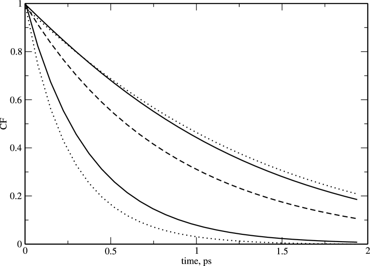
Figure 1: Angular momentum CF $C_{J}(t)$ (full lines), averaged energy $C_{S}(t)$ (dashed lines) and rotational energy CF $C_{E}(t)$ (dotted lines) for algebraic friction (15) with $N=1$, $\xi=1$, and $b=0.29$. The lower CFs are calculated for equilibrium conditions ($\chi=T/T_{ne}=1$) and the upper CFs are computed for hot photofragments ($\chi=0.1$).

We have used Maple 9.5 to numerically solve the FPE (13) with friction (15) and calculate $C_{J}(t)$, $C_{S}(t)$, and $C_{E}(t)$. The results of the calculations are depicted in Fig. 1. As expected, the decay times of all the CFs increase when we approach non-equilibrium conditions (hot photofragments). All the non-equilibrium CFs $C_{J}(t)$, $C_{S}(t)$, and $C_{E}(t)$ differ considerably from each other as well as from their equilibrium counterparts (14). As is clearly seen, $C_{S}(t)$ calculated for hot photofragments deviates significantly from the equilibrium rotational energy CF $C_{E}(t)$ (compare the upper dashed line with the lower dotted line). This is in the agreement with the results of papers, str06 ; str06a which demonstrate inadequacy of the linear response theory in reproducing $C_{S}(t)$ far from equilibrium.

In order to get more insight into the behavior of CFs, it is helpful to consider their integral correlation times

$$\tau_{a}=\int_{0}^{\infty}dtC_{a}(t),\,\,\,\,\,a=J,\,E,\,S.$$ (17)

Now one more argument in favor of choosing algebraic friction (15) is coming: as is shown in the Appendix, we can calculate Eqs. (17) analytically. The results read:

$$\tau_{J}=\frac{1}{\xi}\left\{1+b\,\frac{(2N-1)!!}{\chi^{N}}\right\},$$ (18)

$$\tau_{S}=\frac{1}{2\xi}\left\{1+b\frac{(2N+1)!!}{N+1}\,\,\frac{1/\chi^{N+1}-1}{1/\chi-1}\right\},$$ (19)

$$\tau_{E}=\frac{1}{2\xi}\left\{1+b\frac{(2N+1)!!}{N+1}\,\,\frac{(2N+3)/\chi^{N+1}-1}{3/\chi-1}\right\}.$$ (20)

If $b=0$, then we recover the standard FPE formulas. The presence of $b\neq 0$ causes the increase of the relaxation times.

Eqs. (18)-(20) help us to reveal an important fact. Let us assume that the $J$-dependence of friction (15) is weak, that is $b\ll 1$. If the initial conditions are close to equilibrium ($\chi\sim 1$), then the contribution due to the $J$-dependent friction in Eqs. (18)-(20) is proportional to $b$ and is therefore small. This observation supports the use of the models with constant relaxation rates (the J-diffusion model, gor66 ; rid69 ; McCl77 the standard rotational FPE, hub72 ; McCo ; mor82 ; McCl87 and the Keilson-Storer model gel00 ; BurTe ; kos06 ) for the description of molecular reorientation under equilibrium conditions. Suppose that the initial conditions are highly non-equilibrium, so that the characteristic temperature of the photofragments is much higher than the bath temperature, $\chi=T/T_{ne}\ll 1$. Then the contribution of the second term in Eqs. (18)-(20) is determined by the factor of $b/\chi^{N}$, which is no longer small even if $b\ll 1$.foot5 Thus

$$T_{ne}\sim T/\sqrt[N]{b}$$ (21)

delivers the threshold value of the non-equilibrium temperature (or rotational energy), for which the slowing down of rotational relaxation becomes significant. The existence of such a threshold temperature is clearly demonstrated in Ref.str06a The farther we are from equilibrium (the higher is $\chi$), the stronger is the effect due to the $J$-dependence of friction. This finding corroborates a general paradigm of statistical physics and non-equilibrium thermodynamics, which emphasizes the growing role of fluctuations far from equilibrium.

The above considerations explain why the linear-response theory, which identifies the non-equilibrium averaged rotational energy $C_{S}(t)$ with equilibrium rotational energy fluctuations $C_{E}(t)$, breaks down far from equilibrium. If we are close to equilibrium, then the contribution of the high-$J$ states into rotational relaxation is minor. Thus the equilibrium fluctuations sample adequately the angular momentum exchange between the solute and solvent molecules. If we move far from equilibrium, then rotational relaxation spreads over the high-$J$ states, and equilibrium fluctuations are unable to adequately sample the angular momentum exchange.

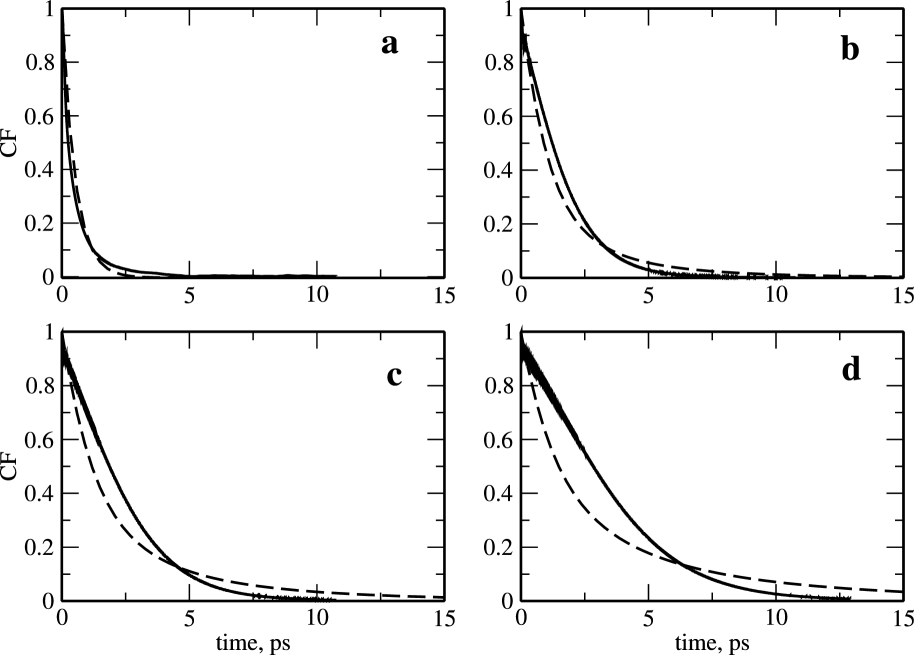
Figure 2: Averaged energy CF $C_{S}(t)$ for $T_{ne}=120$K (a), $1917$K (b), $2395$K (c) and $2875$K (d). Full lines correspond to the molecular dynamics simulations, str06 and dashed lines display the results of the FPE calculations with algebraic friction (15). $N=2$ and the parameters $\xi$ and $b$ are listed in Table 1.

Once Eqs. (18)-(20) are available, we can attempt to make more quantitative comparison of the present theory with the results of simulations reported in. str06 If our approach grasps essential physics of the phenomenon, we shall be able to fit all the simulated $C_{S}(t)$ by a single set of the parameters $N$, $\xi$, and $b$. We have thus proceeded as follows. We have numerically calculated the integral relaxation times of $C_{S}(t)$ simulated at different $T_{ne}$. By combining the obtained dimensionless values of $\tau_{S}$ at equilibrium ($T_{ne}=T=120$K) and at a certain temperature $T_{ne}>T$ we have used Eq. (19) to calculate the corresponding parameters $\xi$ and $b$ for $N=1,\,2$. The results of these calculations are summed up in Table 1. If our approach is self-consistent, the values of $\xi$ and $b$ must be more or less the same for any $T_{ne}$. As is seen from the Table, this is certainly not the case for $N=1$, while the calculations with $N=2$ exhibit a remarkable consistency. Thus we can speculate that the FPE (13) with friction (15) at $N=2$ describes the simulated $C_{S}(t)$ rather adequately. The so calculated $C_{S}(t)$, along with their simulated counterparts str06 are depicted in Fig. 2. The overall agreement is satisfactory, but not perfect. There exists a number of reasons for such a deviation. First, the simulated CFs clearly exhibit short-time non-Markovian behavior. In order to describe this, the present FPE should be generalized to account for memory effects (see, e.g., gel96a ). Such a generalization is necessary, for example, for reproducing the short-time ($\sim 100$fs) coincidence of the simulated $C_{S}(t)$ at different $T_{ne}$.str06 Second, in order to calculate the integral relaxation times (18)-(20) analytically, we have switched to the one-dimensional model, while the actual description for linear photofragments must be two-dimensional. Third, as is well known, the FPE itself may not be very good for reproducing rotational relaxation in liquids LB84 , so that more refine approaches might be necessary. The present paper undertakes the first step toward understanding non-equilibrium rotational relaxation. The message is as follows: the friction, or the collision frequency, or the relaxation rate must be taken $J$-dependent in order to adequately describe rotational relaxation under highly non-equilibrium conditions.

IV Conclusion

Recently, the groups of Bradforth and Stratt have published the results of the combined theoretical and experimental study of rotational relaxation of CN-photofragments in a condensed phase. str06 ; str06a They show via molecular dynamics simulations that the time evolution of the averaged rotational energy, $C_{S}(t)$, (i) slows down dramatically with the increase of the rotational temperature of the incipient photofragments and (ii) deviates significantly from the equilibrium rotational energy CF, $C_{E}(t)$, manifesting the linear response breakdown. To comprehend and explain this unusual behavior, we have developed a theory of rotational relaxation under non-equilibrium conditions, by extending the standard FPE approach to account for angular momentum dependent friction. We have calculated the angular momentum CF $C_{J}(t)$, as well as $C_{S}(t)$ and $C_{E}(t)$, and compared them with their simulated counterparts. str06 We have shown that $J$-dependence of rotational friction is responsible for the observed slowing down of rotational relaxation and failure of the linear response description, provided the effective non-equilibrium rotational temperature exceeds the threshold value (21). The farther the system is from the equilibrium, the stronger is the effect.

Appendix A Calculation of the integral relaxation times

We start from the one-dimensional FPE with the angular momentum dependent friction $\xi(J)$,

$$\partial_{t}\rho(J,t)=\partial_{J}\xi(J)(J+\partial_{J})\rho(J,t).$$ (22)

Evidently, a CF of the functions $A(J)$ and $B(J)$ can be evaluated via Eq. (22) as follows:

$$C_{AB}(t)=\left\langle A(J)B(J(t))\right\rangle_{ne}-\left\langle A(J))\right\rangle_{ne}\left\langle B(J)\right\rangle_{B}=\int_{-\infty}^{\infty}dJB(J)\rho(J,t)$$ (23)

(the notation is identical to that used in Eqs. (9)-(11)). The initial condition to Eq. (22) reads then:

$$\rho(J,0)=A(J)\rho_{ne}(J)-\left\langle A(J)\right\rangle_{ne}\rho_{B}(J).$$

Here the initial non-equilibrium distribution is determined by Eq. (16), and the Boltzmann equilibrium distribution is defined via Eq. (5) with $d=1$. Let

$$\tau_{AB}=\int_{0}^{\infty}dt\left\{\left\langle A(J)B(J(t))\right\rangle_{ne}-\left\langle A(J))\right\rangle_{ne}\left\langle B(J)\right\rangle_{B}\right\}$$

be the integral relaxation time for the above CF. Then, integrating Eq. (22) over time and introducing the quantity

$$\eta(J)=\int_{0}^{\infty}dt\rho(J,t),$$

we can express $\tau_{AB}$ through $\eta(J)$ as follows:

$$\tau_{AB}=\int_{-\infty}^{\infty}dJB(J)\eta(J).$$ (24)

Here $\eta(J)$ obeys the differential equation

$$-\left\{A(J)\rho_{ne}(J)-\left\langle A(J)\right\rangle_{ne}\rho_{B}(J)\right\}=\partial_{J}\xi(J)(J+\partial_{J})\eta(J).$$ (25)

Eq. (25) must be solved with the boundary conditions $\eta(\pm\infty)=0$. It is convenient to introduce the quantity $\widetilde{\eta}(J)$ via the expression

$$\eta(J)\equiv\widetilde{\eta}(J)\rho_{B}(J).$$ (26)

Upon the insertion of the above equation into Eq. (25), we get:

$$-\frac{1}{\rho_{B}(J)\xi(J)}\int_{0}^{J}dJ^{\prime}\left\{A(J^{\prime})\rho_{ne}(J^{\prime})-\left\langle A(J)\right\rangle_{ne}\rho_{B}(J^{\prime})\right\}=\partial_{J}\widetilde{\eta}(J)$$ (27)

(the integration limits have been chosen to comply with the boundary conditions $\eta(\pm\infty)=0$). As is seen, Eq. (27) can be integrated, in principle, for any $\rho_{ne}(J)$, $\xi(J)$, and $A(J)$. To simplify the subsequent presentation, we shall limit ourselves to the case when

$$B(J)=J^{m},m=1\,\textrm{or}\,2.$$ (28)

Inserting this expression into Eq. (24), using the definition (26) and integrating by parts yields then

$$\tau_{AB}=\int_{-\infty}^{\infty}dJJ^{m-1}\rho_{B}(J)\partial_{J}\widetilde{\eta}(J),\,\,\,m=1\,\textrm{or}\,2.$$ (29)

Combining Eqs. (27) and (29), we get:

$$\tau_{AB}=-\int_{-\infty}^{\infty}dJJ^{m-1}\frac{1}{\xi(J)}\int_{0}^{J}dJ^{\prime}\left\{A(J^{\prime})\rho_{ne}(J^{\prime})-\left\langle A(J)\right\rangle_{ne}\rho_{B}(J^{\prime})\right\},\,\,\,m=1\,\textrm{or}\,2.$$ (30)

Using the explicit form (15) of the angular momentum friction and integrating Eq. (30) by parts gives, finally:

$$\tau_{AB}=\frac{1}{\xi}\int_{-\infty}^{\infty}dJ\left(\frac{J^{m}}{m}+b\frac{J^{m+2N}}{m+2N}\right)\left\{A(J)\rho_{ne}(J)-\left\langle A(J)\right\rangle_{ne}\rho_{B}(J)\right\},\,\,\,m=1\,\textrm{or}\,2.$$ (31)

This is the formula which has been used for the calculation of integral relaxation times (18)-(20).

Table 1: The dimensionless parameters $\xi$ and $b$ calculated via Eq. (19) from the integral relaxation times $\tau_{S}$ (given in units of $\tau_{r}$) simulated at different temperatures $T_{ne}$ (in K). Integral relaxation time $\tau_{S}=1.77$ at equilibrium temperature $120$K.

Simulationstr06			$N=1$			$N=2$
$T_{ne}$	$\tau_{S}$		$\xi$	$b$		$\xi$	$b$
$1917$	$5.29$		$0.39$	$0.12$		$0.29$	$0.0015$
$2395$	$7.73$		$0.44$	$0.18$		$0.29$	$0.0017$
$2875$	$11.25$		$0.53$	$0.29$		$0.29$	$0.0018$

References

- (1) J. S. Baskin and A. Zewail, J. Phys. Chem. 98, 3337 (1994).
- (2) J. S. Baskin and A. H. Zewail, J. Phys. Chem. A 105, 3680 (2001).
- (3) B. Locke, T. Lian, and R. M. Hochstrasser, Chem. Phys. 158, 409 (1991).
- (4) M. Lim, T. A. Jackson, and P. A. Anfinrud, J. Chem. Phys. 102, 4355 (1995).
- (5) M. Lim, T. A. Jackson, and P. A. Anfinrud, J. Am. Chem. Soc. 126, 7946 (2004).
- (6) S. Kim and M. Lim, J. Am. Chem. Soc. 127, 5786 (2005).
- (7) J. Helbing, K. Nienhaus, G. U. Nienhaus, P. Hamm, J. Chem. Phys. 122, 124505 (2005).
- (8) U. Banin and S. Ruhman, J. Chem. Phys. 98, 4391 (1993).
- (9) E. Lenderink, K. Duppen, and D. A. Wiersma, Chem. Phys. Lett. 211, 503 (1993).
- (10) E. Lenderink, K. Duppen, F. P. X. Everdij, J. Marvi, R. Torre, and D. A. Wiersma, J. Phys. Chem. 100, 7822 (1996).
- (11) C. Wan, M. Gupta, and A. Zewail, Chem. Phys. Lett. 256, 279 (1996).
- (12) S. Gnanakaran, M. Lim, N. Pugliano, M. Volk, and R. M. Hochstrasser, J. Phys.: Condense Matter 8, 9201 (1996).
- (13) M. Volk, S. Gnanakaran, E. Gooding, Y. Kholodenko, N. Pugliano, and R. M. Hochstrasser, J. Phys. Chem. A. 101, 638 (1997).
- (14) M. Lim, S. Gnanakaran, and R. M. Hochstrasser, J. Chem. Phys. 106, 3485 (1997).
- (15) T. Kühne and P. Vöhringer, J. Phys. Chem. A 102, 4177 (1998).
- (16) S. Hess, H. Bürsing, and P. Vöhringer, J. Chem. Phys. 111, 5461 (1999).
- (17) M. Volk, J. Phys. Chem. A 103, 5621 (1999).
- (18) S. Hess, H. Hippler, T. Kühne, and P. Vöhringer, J. Phys. Chem. A 103, 5622 (1999).
- (19) H. Bürsing, J. Lindner, S. Hess, and P. Vöhringer, Appl. Phys. B. 71, 411 (2000).
- (20) H. Bürsing and P. Vöhringer, PCCP 2, 73 (2000).
- (21) H. Fidder, F. Tschirschwitz, O. Dühr, and E. T. J. Nibbering, J. Chem. Phys. 114, 6781 (2001).
- (22) A. C. Moskun and S. E. Bradforth, J. Chem. Phys. 119, 4500 (2003).
- (23) J.E. Straub and M. Karplus, Chem. Phys. 158, 221 (1991).
- (24) I. Benjamin and K. R. Wilson, J. Chem. Phys. 90, 4176 (1989).
- (25) I. I. Benjamin, U. Banin and S. Ruhman, J. Chem. Phys. 98, 8337 (1993).
- (26) I. Benjamin, J. Chem. Phys. 103, 2459 (1996).
- (27) A. I. Krylov and B. B. Gerber, J. Chem. Phys. 100, 4242 (1994).
- (28) A. P. Blokhin and M. F. Gelin, Chem. Phys. 252, 323 (2000).
- (29) M. F. Gelin, J. Mol. Liq. 93, 51 (2001).
- (30) A. P. Blokhin and M. F. Gelin, PCCP 4, 3356 (2002).
- (31) A. S. Moskun, A. E. Jailaubekov, S. E. Bradforth, G. Tao, and R. M. Stratt, Science 311, 1907 (2006).
- (32) G. Tao and R. M. Stratt, J. Chem. Phys. 125, 114501 (2006).
- (33) This assumption, in principle, can be relaxed but it is adequate. Since photodissociation is normally quite fast (hundreds of femtosecondszew94 ; zew01 ) on the rotational dynamics timescale, the ensemble of photofragments can be thought of as being instantaneously injected into the equilibrium heat bath.
- (34) L.-P. Hwang and J. H. Freed, J. Chem. Phys. 63, 118 (1975).
- (35) G. T. Evans, Mol. Phys. 36, 65 (1978).
- (36) A. P. Blokhin and M. F. Gelin, Physica A 251, 469 (1998).
- (37) R. G. Gordon, J. Chem. Phys. 44, 1830 (1966).
- (38) M. Fixman and K. Rider, J. Chem. Phys. 51, 2425 (1969).
- (39) R. E. D. McClung, Adv. Mol. Rel. Int. Proc. 10, 83 (1977).
- (40) P. S. Hubbard, Phys. Rev. A. 6, 2421 (1972).
- (41) G. W. Ford, J. T. Lewis and J. McConnell, Phys. Rev. A. 19, 907 (1979).
- (42) A. Morita, J. Chem. Phys. 76, 3198 (1982).
- (43) D. H. Lee and R. E. D. McClung, Chem. Phys. 112, 23 (1987).
- (44) A. I. Burshtein, L. M. Strekalov and S. I. Temkin, Sov. Phys. JETP 39, 433 (1974).
- (45) A. I. Burshtein and S. I. Temkin. Spectroscopy of Molecular Rotations in Gases and Liquids (Cambridge University Press, Cambridge, 1994).
- (46) M. F. Gelin and D. S. Kosov, J. Chem. Phys. 124, 144514 (2006).
- (47) In this case, the eigenfunctions (see ref. BurTe ), being the Hermite polynomials.
- (48) M. P. Allen, G. T. Evans, D. Frenkel, B. M. Mulder, Adv. Chem. Phys. 83, 89 (1993).
- (49) R. E. D. McClung, J. Chem. Phys. 57, 5478 (1972).
- (50) C. Dreyfus, C. Breuillard, N. T. Tai, and R. Ouillon. Chem. Phys. Lett. 62, 246 (1979).
- (51) S. Dattagupta and A. K. Sood, Pramana 13, 423 (1979).
- (52) G. Wylie, Phys. Rep. 61, 327 (1980).
- (53) A. P. Blokhin and M. F. Gelin, Khim. Fiz. 17, No 12, 108 (1998).
- (54) Strictly speaking, the averaged rotational energy CF, , is identically zero under equilibrium conditions (). However, the normalized CF , as defined by Eq. (10), yields in the limit .
- (55) H. Risken. The Fokker-Planck Equation (Springer, Berlin, 1984).
- (56) U. Erdmann, W. Ebeling, L. Schimansky-Geier, and F. Schweitzer, Eur. Phys. J. B 15, 105 (2000).
- (57) M. G. Kurnikova, D. H. Waldeck and R. D. Coalson, J. Chem. Phys. 105, 628 (1996).
- (58) R. M. Stratt and M. Maroncelli, J. Phys. Chem. 100, 12981 (1996).
- (59) P. V. Kumar and M. Maroncelli, J. Chem. Phys. 112, 5370 (2000).
- (60) B. Bagchi and R. Biswas, Adv. Chem. Phys. 109, 207 (1999).
- (61) J. Jang and R. M. Stratt, J. Chem. Phys. 112, 7524 and 7538 (2000).
- (62) There is, perhaps, no good reason to consider high values of in Eq. (15), so that the first few are meaningful.
- (63) A more physically justified parametrization of can be found in Refs. zew94 ; gel00 ; gel01 ; gel02
- (64) Note that Eqs. (18)-(20) predict that rotational relaxation in non-equilibrium cold ensembles () is faster than in equilibrium ensembles (). Since the parameter is assumed to be small, this effect is not so pronounced, in general.
- (65) A. P. Blokhin and M. F. Gelin, Physica A 229, 501 (1996).
- (66) R. M. Lynden-Bell, in Molecular liquids, edited by A. J. Barnes, W. J. Orville-Thomas and J. Yarwood (NATO ASI Series C, V. 135, 1984), P. 501.