Anomalous kinetics and transport from 1D self–consistent mode–coupling theory

Abstract

We study the dynamics of long-wavelength fluctuations in one-dimensional (1D) many-particle systems as described by self-consistent mode-coupling theory. The corresponding nonlinear integro-differential equations for the relevant correlators are solved analytically and checked numerically. In particular, we find that the memory functions exhibit a power-law decay accompanied by relatively fast oscillations. Furthermore, the scaling behaviour and, correspondingly, the universality class depends on the order of the leading nonlinear term. In the cubic case, both viscosity and thermal conductivity diverge in the thermodynamic limit. In the quartic case, a faster decay of the memory functions leads to a finite viscosity, while thermal conductivity exhibits an even faster divergence. Finally, our analysis puts on a more firm basis the previously conjectured connection between anomalous heat conductivity and anomalous diffusion.

Keywords: Transport processes / heat transfer (Theory)

1 Introduction

Numerical and theoretical studies of transport in reduced spatial dimensions (1 and 2D) have revealed that unexpected properties of matter may emerge with respect to the standard features of 3D systems. This fact, combined with the possibility of designing and manipulating matter at the nanoscale, unveals the possibility of exploring new physical phenomena and applications. Preliminary indications about anomalous hydrodynamic behaviors were discovered in the context of non–equilibrium statistical mechanics by the appearance of long–time tails in fluid models [1, 2]. In fact, there are many instances showing that microscopic models of hydrodynamics can be affected by serious pathologies. For the sake of an example, we mention the anomalous scaling of Rayleigh and Brillouin peak widths in the hydrodynamic limit detected in the 1D Lennard–Jones fluid [3, 4]. Another instance is the divergence of viscosity in cellular automata fluids [5] that may however be due their peculiar features.

On the one hand, the breakdown of phenomenological constitutive laws of hydrodynamics, yielding ill-defined transport coefficients, could be viewed as a drawback for the adopted models and theoretical approaches. On the other hand, it is nowadays widely recognized that anomalous transport is a documented effect rather than an accident due to the oversimplification of theoretical models. Typical examples are single-filing systems, where particle diffusion does not follow Fick’s law [6], and the enhancement of vibrational energy transmission in quasi-$1D$ systems, such as polymers [7] or individual carbon nanotubes [8].

Within this general context, one of the issues that attracted a renewed interest in the last decade is the problem of anomalous heat conduction in low-dimensional many-particle systems [9, 10]. In this case, the anomalous features amount to the divergence of the finite-size heat conductivity $\kappa(L)\propto L^{\alpha}$ in the limit $L\to\infty$ and, correspondingly, to a nonintegrable decay of equilibrium correlations of the energy current (the Green-Kubo integrand), $\langle J(t)J(0)\rangle\propto t^{-(1-\alpha)}$($0\leq\alpha<1$) for long times $t\to\infty$. Numerical studies  [11] and theoretical arguments [12] indicate that anomalies should occur generically in 1 and 2D, whenever momentum is conserved. In particular, a great deal of studies have been devoted to the prediction of the exponent $\alpha$ for a twofold reason. On a basic ground, one is interested in identifying the universality classes and the relevant symmetries possibly identifying them. From a practical point of view, an accurate prediction of the scaling behaviour allows determining heat conductivity in finite systems – a crucial issue for the comparison with experiments.

Despite many efforts, the theoretical scenario is still controversial. The first attempt of tackling the problem was based on arguments derived from the Mode-Coupling Theory (MCT). This approach proved quite powerful for the estimate of long-time tails in fluids [1] and for describing the glass transition [13]. In 1D models [14], the MCT prediction was $\alpha=2/5$ [10, 15], very close to the numerical values [11]. This estimate was later criticized as inconsistent in [12], where renormalization group arguments were instead shown to yield $\alpha=1/3$. Nevertheless, the 2/5 value has been later derived both from a kinetic-theory calculation for the quartic Fermi–Pasta–Ulam (FPU-$\beta$) model [16] and from a solution of the MCT by means of an ad hoc Ansatz [17]. It was thereby conjectured [17] that 2/5 is found for a purely longitudinal dynamics, while a crossover towards 1/3 is to be observed only in the presence of a coupling to transversal motion. Unfortunately, the accuracy of numerical simulations is generally insufficient to disentangle the whole picture. Without pretending to give a full account of the various numerical results (see [18] for a recent account), it is worth mentioning that, while for some models like the so called hard–point gas [19] the data is compatible with the prediction $\alpha=1/3$ [20], some other cases show huge deviations. For example, in the purely quartic FPU model, $\alpha$ is definitely larger than 1/3 and definitely closer to 2/5 [21]. The situation is even more controversial in 2D, where MCT predicts a logarithmic divergence [22] that is not yet confirmed by numerical simulations.

For all the above reasons, we decided to reconsider MCT to clarify the origin of the reported discrepancies. Typically, MCT is implemented by imposing an ad-hoc Ansatz for the dependence of the hydrodynamic propagator and of the memory kernel on the space and time variables. In this paper, following  [23], we find an exact self-consistent solution of the MCT equations, without any a priori assumption on the form of the solution. The resulting scaling behavour differs from that one proposed in [17]. Moreover, the asymptotic behaviour turns out to depend on the order of the leading nonlinearity in the interaction potential. Indeed, we find that cubic and quartic nonlinearities are characterized by $\alpha=1/3$, and $1/2$, respectively. Remarkably, an even more striking difference is exhibited by viscosity which appears to diverge in the former case, while is finite in the latter one.

The structure of the paper is as follows. In Section 2 we review the mode–coupling equations and discuss their physical meaning. Section 3 is devoted to the solution when the leading nonlinearity is cubic, while in Section 4 we discuss how the solutions change in the presence of a leading quartic nonlinearity. In Section 5, the knowledge of the mode–coupling solutions is exploited to determine the value of the scaling exponent $\alpha$, by estimating the heat current correlation function. Final remarks and future perspectives of this approach are reported in the conclusions.

2 MCT equations

The introduction of suitable stochastic equations ruling the dynamics of the relevant variables is rather customary to describe the relaxation close to equilibrium [24]. The idea consists in concentrating on the effective motion of the “slow” observables, i.e. in changing level of description. The general strategy amounts to projecting the original equations onto a suitable subspace and eventually leads to linear non-Markovian equations. The memory term determines the relaxation properties. Whenever a sharp separation of time scales exist, the equations reduce to their Markovian limit.

Let us consider the simplest one-dimensional version of the self-consistent MCT. For definiteness, we consider a Hamiltonian chain of oscillators, interacting through a generic nearest-neighbour coupling potential $V$, whose Taylor expansion around equilibrium is written as

$$V(y)\;=\;{1\over 2}\,y^{2}\,+\,{1\over 3}g_{3}\,y^{3}\,+\,{1\over 4}g_{4}\,y^{4}\,+\,\ldots$$ (1)

The variable $y$ is a short-hand notation for the difference of nearest neighbour displacement fields $(u_{i+1}-u_{i})$, with the integer index $i$ labelling the lattice sites. Besides the conservation of total energy, such a kind of interaction implies also the conservation of total momentum due to space-translation invariance.

The main observable we are interested in is the normalized correlator $G(q,t)=\langle Q^{*}(q,t)Q(q,0)\rangle/\langle|Q(q)|^{2}\rangle$, where $Q(q,t)$ is the Fourier transform of the displacement field $u_{i}(t)$. By assuming periodic boundary conditions for a chain made of $N$ sites, the wavenumber is given by $q=2\pi k/N$, with $-N/2+1\leq k\leq N/2$. Notice also that $G(q,t)=G(-q,t)$. We simplify the notation by setting to unity the particle mass, the lattice spacing and the bare sound velocity. The equations for the correlator $G(q,t)$ then read  [25, 15]

$${\ddot{G}}(q,t)+\varepsilon\int_{0}^{t}\Gamma(q,t-s){\dot{G}}(q,s)\,ds+{\omega}^{2}(q)G(q,t)=0$$

where the memory kernel $\Gamma(q,t)$ is proportional to $\langle\mathcal{F}(q,t)\mathcal{F}(q,0)\rangle$ with $\mathcal{F}(q)$ being the nonlinear part of the force between particles. Equations (2) must be solved with the initial conditions $G(q,0)=1$ and $\dot{G}(q,0)=0$. Equations  (2) are exact and they are derived within the well–known Mori–Zwanzig projection approach [24].

The mode–coupling approach basically amounts to replacing the exact memory function $\Gamma$ with an approximate one, where higher–orders correlators are written in terms of the $G(q,t)$. This yield a closed system of nonlinear integro–differential equations. For potentials like (1) this has been worked out in detail in references  [25, 15]. Both the coupling constant $\varepsilon$ and the frequency $\omega(q)$ are temperature-dependent input parameters, which should be computed independently by numerical simulations or approximate analytical estimates [25, 15]. For the aims of the present work, we may restrict ourselves to considering their bare values, obtained in the harmonic approximation. In the adopted dimensionless units they read $\varepsilon={3g_{3}^{2}k_{B}T/2\pi}$ and $\omega(q)=2|\sin{q\over 2}|$. Of course, the actual renormalized values are needed for a quantitative comparison with specific models.

To understand the physical interpretation of equation (2), let us first assume that a Markovian approximation holds i.e. we can replace the memory function by a Dirac delta. In the small wavenumber limit $q\to 0$ they reduce to

$${\ddot{G}}(q,t)+\eta q^{2}{\dot{G}}(q,t)+c^{2}q^{2}G(q,t)\;=\;0$$ (2)

where, for the sake of clarity, we have reintroduced the sound velocity $c$. Notice that the validity of (2) rests on the fact that $\Gamma$ exhibits a fast decay and that its time integral is finite. This equation describes the response of an elastic string at finite temperature as predicted by linear elasticity theory [26] for the macroscopic displacement field $u(x,t)$

$$\ddot{u}-c^{2}\partial_{x}^{2}u-\eta\partial_{x}^{2}\dot{u}\;=\;0\quad.$$ (3)

Here $\eta$ is a suitable viscosity coefficient and describes the internal irreversible processes of the elastic string (i.e. the absorption of “sound” waves). We anticipate that one of our results is precisely that (generically) the above approximation does not hold and that long–range memory effects must be retained [27].

3 Cubic nonlinearities

In the generic case in which $g_{3}$ in equation (1) is different from zero, the lowest-order mode coupling approximation of the memory kernel turns out to be [25, 15]

$$\Gamma(q,t)=\,\omega^{2}(q)\,\frac{2\pi}{N}\sum_{p+p^{\prime}-q=0,\pm\pi}\,G(p,t)G(p^{\prime},t)\quad.$$ (4)

Equation (2) along with (4) are now a closed system that has to be solved self-consistently. The integral terms contain products of the form $GG\dot{G}$ and we thus refer to this case as to the cubic nonlinearity.

3.1 Analytical results

Direct numerical simulations [15] indicate that for small wavenumbers nonlinear and nonlocal losses in equation (2) are small compared with the oscillatory terms. This suggests splitting the $G$ dynamics into phase and amplitude evolution,

$$G(q,t)\;=\;C(q,t)e^{i\omega(q)t}+c.c.$$ (5)

As already shown in [23], this Ansatz allows reducing the dynamics to a first order equation for $C(q,t)$ and, in turn, determining the scaling behavior of the correlators. Let us start by rearranging the expression for $\Gamma(q,t)$. By inserting equation (5) into (4), we obtain

$$\Gamma(q,t) \;=\; \omega^{2}(q)\int_{-\pi}^{\pi}dp\,\Big{[}C(p,t)C(q-p,t)e^{i[\omega(p)+\omega(q-p)]t}$$

$$+C(p,t)C^{\ast}(q-p,t)e^{i[\omega(p)-\omega(q-p)]t}\Big{]}\,+\,c.c.$$

where the sum in (2) has been replaced by an integral, since we are interested in the thermodynamic limit $N=\infty$. For small $q$-values, which are, by the way, responsible for the asymptotic behavior, the above equation reduces to

$$\Gamma(q,t) \;\approx \;q^{2}\int_{-\pi}^{\pi}dp\,\Big{[}C(p,t)C(q-p,t)e^{2i\omega(p)t}$$

$$+C(p,t)C^{\ast}(q-p,t)e^{-i\omega^{\prime}(p)qt}\Big{]}\,+\,c.c.$$

where $\omega^{\prime}(p)=\frac{d\omega}{dp}$. The first term in the r.h.s. and its complex conjugate are negligible because of the rapidly varying phase. By further neglecting the dependence of the sound velocity on $q$ (i.e. $\omega^{\prime}(p)\approx 1$), one finds that $\Gamma(q,t)$ has the following structure,

$$\Gamma(q,t)\;=\;M(q,t)e^{iqt}\,+\,c.\,c.$$ (8)

where

$$M(q,t)\equiv q^{2}\int_{-\pi}^{\pi}dp\,C^{\ast}(p,t)C(q-p,t)$$ (9)

is the kernel in the new description. Upon substituting equation (8) and (5) into (2), one obtains, in the slowly varying envelope approximation, $\dot{C}\ll qC$,

$$2\dot{C}(q,t)+\varepsilon\int_{0}^{t}\,dt^{\prime}\,M(q,t-t^{\prime})C(q,t^{\prime})\;=\;0$$ (10)

and a similar expression for $C^{*}$.

Equation (10) have been obtained after discarding the second order time derivative of $C(q,t)$ as well as the integral term proportional to $\dot{C}$, besides all rapidly rotating terms. The validity of this approximation is related to the separation between the decay rate of $C(q,t)$ and $\omega(q)$; its correctness will be cheked a posteriori, after discussing the scaling behaviour of $C(q,t)$. Notice also that in this approximation, Umklapp processes do not contribute: it is in fact well known that they are negligible for long–wavelength phonons in 1D  [11].

Having transformed the second order differential equation into a first order one for $C(q,t)$, it is now possible to develop a scaling analysis for the dependence of $C$ on $q$ and $t$, owing to the homogeneous structure of the resulting equation (see also [28], where a similar equation was investigated). More precisely, one can easily verify that the following Ansatz holds,

$$C(q,t)=g(\sqrt{\varepsilon}tq^{3/2})\quad,\quad M(q,t)=q^{3}f(\sqrt{\varepsilon}tq^{3/2}).$$ (11)

This shows that the decay rate for the evolution of $C(q,t)$ is given by $q^{3/2}\sqrt{\varepsilon}$. Since the corresponding rate for the phase factor is $q$, one can conclude that amplitude and phase dynamics are increasingly separated for $q\to 0$. High $q$-values ($q\approx 1$) are those for which the slowly varying envelope approximation is less accurate. However, if $\varepsilon$ is small enough, such modes are correctly described, too. This has been checked in the numerical solution of equation (2) (see the following subsection).

The functions $f$ and $g$ can be determined by substituting the previous expressions into (10) and(9). Upon setting $x=\sqrt{\varepsilon}tq^{3/2}$, one obtains the equation

$$\frac{dg}{dx}=-\int_{0}^{x}dy\,f(x-y)g(y)$$ (12)

$$f(x)=x^{-2/3}\int_{-\infty}^{+\infty}dyg^{\ast}(\mid x^{2/3}-y\mid^{3/2})g(y^{3/2})\quad,$$ (13)

where the integral in (9) has be extended to infinity.

The asymptotic behaviour for $x\to 0$ can be determined analytically. Actually, one can neglect the dependence on $x$ in the integral appearing in (13), thus obtaining

$$f(x)\;=\;\frac{a}{x^{2/3}}$$ (14)

where

$$a=\int_{-\infty}^{+\infty}dy|g|^{2}(y^{3/2})$$ (15)

which implies that

$$M(q,t)=\frac{a}{\varepsilon^{1/3}}\frac{q^{2}}{t^{2/3}}$$ (16)

By replacing equation (14) into (12) and introducing the dummy variable $z=x-y$, one finds

$$\frac{dg}{dx}=-a\int_{0}^{x}dz\frac{g(x-z)}{z^{2/3}}=-3agx^{1/3}-\frac{3}{2}a\frac{dg}{dx}x^{4/3}+\ldots$$ (17)

In the small-$x$ limit, the last term in the r.h.s. is negligible with respect to the term in the l.h.s. After solving the resulting differential equation one obtains,

$$g(x)\;=\;\frac{1}{2}\exp\Big{(}-{9ax^{4/3}\over 4}\Big{)}$$ (18)

where the multiplicative factor has been determined by imposing the normalization condition $G(0)=1$.

Under the approximation that expression (14) holds for every $x$, one can exactly solve equation (12) by Laplace transformation. As a result, one obtains

$$C(q,z)\;=\;\frac{iz^{1/3}}{iz^{4/3}+aq^{2}}\quad.$$ (19)

This expression is precisely the Laplace transform of the Mittag-Leffler function $E_{\mu}(-(\lambda t)^{\mu})$ [30, 29] for $\mu=4/3$ and $\lambda=(aq^{2})^{3/4}$. The function $E_{\mu}$ interpolates between stretched exponential and power-law decays (see Appendix B in [29]). The asymptotic form for small values of the function argument yields the same dependence for $C$ (see the first of equations (11)). This observation suggests that the effective evolution of fluctuations should be represented by the fractional differential equation

$${\partial^{\mu}\over\partial t^{\mu}}C(q,t)+\lambda^{\mu}C(q,t)\;=\;0.$$ (20)

The case of interest here ($1<\mu\leq 2$) corresponds to the so–called fractional oscillations [30]. It should be emphasized that in the present context, memory arises as a genuine many-body effect and is not postulated a priori.

3.2 Numerical analysis

To assess the validity of the above calculation, we have numerically integrated equations (2) by the Euler method for the original dispersion relation $\omega(q)$ and different values of $\varepsilon$. We have verified that a time step $\Delta t=0.01$ guarantees a good numerical accuracy over the explored time range. The Fourier transform $G(q,\omega)$ is plotted in figure 1 for three different $q$-values versus $\omega-\omega_{M}(q)$, where $\omega_{M}(q)$ is the frequency corresponding to the maximal value $G_{M}$ of the spectrum (this is equivalent to removing the oscillating component from $G(q,t)$). Furthermore, in order to test relation (11), the vertical axis is scaled to the maximum $G$-value, while the frequencies are divided by the half–width $\gamma(q)$ at half of the maximum height. This latter quantity can be interpreted as the inverse lifetime of fluctuations of wavenumber $q$. The good data collapse confirms the existence of a scaling regime. Moreover, the numerical data is compared with the approximate analytical expression, obtained by Fourier transforming the function defined in (11) and (18) (solid curve). The overall agreement is excellent; there are only minor deviations for small values of $\omega-\omega_{M}$ where (18) is not strictly applicable. Moreover, in the inset of figure 1, where the same curves are plotted using doubly logarithmic scales, one can see that the lineshapes follow the predicted power-law, $\omega^{-7/3}$, over a wide range of frequencies. This scaling has been deduced by Fourier transforming $g(x)$ in equation (18).

In figure 2 we show that $\gamma(q)$ is indeed proportional to $\sqrt{\varepsilon}\,q^{3/2}$. It is noteworthy to remark that the agreement is very good also also for a relatively large value of the coupling constant such as $\varepsilon=1$, although the slowly varying envelope approximation is not correct for large wavenumbers. The deviations observed at small $q$-values for small couplings are due to the very slow convergence in time. Better performances could be obtained by increasing both $N$ and the integration time ($10^{4}$, in our units), however, well beyond our current capabilities. Finally, we have plotted the Fourier tranform of the memory function (see figure 3) to check its scaling behaviour. By Fourier transforming equation (16), one finds a behaviour like $\omega^{-1/3}$ which is reasonably well reproduced in figure 3). Once again, in order to obtain a larger scaling range, it would be necessary to consider significantly larger system sizes.

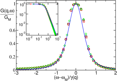
Figure 1: Fourier transform $G(q,\omega)$ of the correlation functions for $\varepsilon=1$, $N=2000$ and the three wavenumbers, $q=\pi/100$ (circles), $2\pi/100$ (squares), and $3\pi/100$ (diamonds). The solid line corresponds to the approximate analytic theory, i.e. it is obtained by Fourier transforming the function $C(q,t)$ defined in (11,18). The same curves are plotted in the inset in log-log scales, where only positive frequencies are shown.

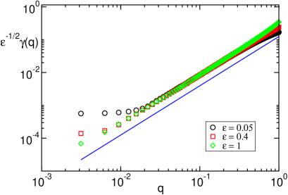
Figure 2: Scaling of the linewidth $\gamma(q)$ of $G(q,\omega)$ with $q$ for three different values of the coupling constant $\varepsilon$ and $N=2000$. The solid line corresponding to the expected power law $q^{3/2}$ is plotted for reference.

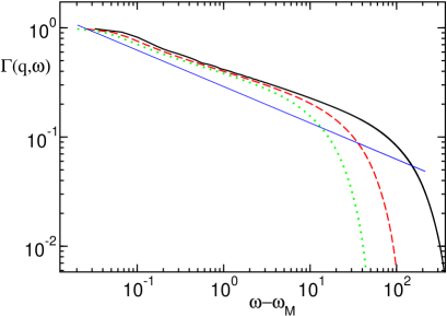
Figure 3: Fourier transform of the memory function $\Gamma(q,\omega)$ for the same parameter values as in figure 1 and for three wavenumbers, namely, $\pi/100$ (solid line), $2\pi/100$ (dashed line), and $3\pi/100$ (dotted line). The $\omega$ axis is suitably shifted in order to get rid of the oscillatory peak at frequency $q$, so that $\Gamma(q,\omega)$ reduces to $M(q,\omega)$. For comparison, the expected power-law $\omega^{-1/3}$ is also presented (thin solid line).

Making use of equations  (11,18), it can be shown that the memory function $\Gamma$ contains terms of the form $q^{2}\,e^{\pm iqt}/t^{2/3}$, i.e. it oscillates with a power–law envelope. Accordingly, its Laplace trasform has branch-cut singularities of the form $q^{2}/(z\pm q)^{\frac{1}{3}}$. This finding is not consistent with the heuristic assumption made in [14, 15] and the result of [17], where simplified MCT equations were solved with the Ansatz $\Gamma(q,z)=q^{2}\mathcal{V}(z)$. In addition, the numerical solution does not show any signature of the $q^{2}/z^{1/3}$ dependence found in  [17]. For instance, it would imply a peak at $\omega=0$ in the spectrum of $\Gamma$ which is, instead, absent in our data.

4 Quartic nonlinearities

In this section, we turn our attention to the case of a vanishing $g_{3}$. This the case of symmetric potentials (with respect to the equilibrium position), but it is more general than that. The kernel of the mode coupling equations writes in this case

$$\Gamma(q,t)=\,\omega^{2}(q)\,\Big{(}\frac{2\pi}{N}\Big{)}^{2}\sum_{p+p^{\prime}+p^{\prime\prime}-q=0,\pm\pi}\,G(p,t)G(p^{\prime},t)G(p^{\prime\prime},t)\quad.$$ (21)

Equation (2) is still formally valid as it stands, with the (bare) coupling constant now given by $\varepsilon={15(g_{4}\,k_{B}T/2\pi)^{2}}$ [15].

4.1 Analytical results

One can repeat the same analysis performed for the cubic case. By substituting expression (5) into (21), we must now deal with a double integral,

$$\Gamma(q,t)=\omega^{2}(q)\int_{-\pi}^{\pi}dp\int_{-\pi}^{\pi}dp^{\prime}\Big{[}C(p,t)C(p^{\prime},t)C(q-p-p^{\prime},t)e^{i[\omega(p)+\omega(p^{\prime})+\omega(q-p-p^{\prime})]t}$$

$$+C(p,t)C(p^{\prime},t)C^{\ast}(q-p-p^{\prime},t)e^{i[\omega(p)+\omega(p^{\prime})-\omega(q-p-p^{\prime})]t}$$

$$+C(p,t)C^{\ast}(p^{\prime},t)C(q-p-p^{\prime},t)e^{i[\omega(p)-\omega(p^{\prime})+\omega(q-p-p^{\prime})]t}$$

$$+C(p,t)C^{\ast}(p^{\prime},t)C^{\ast}(q-p-p^{\prime},t)e^{i[\omega(p)-\omega(p^{\prime})-\omega(q-p-p^{\prime})]t}+c.c.\Big{]}\quad.$$ (22)

By neglecting the non-resonant terms in the limit $q\rightarrow 0$, the above expression simplifies to

$$\Gamma(q,t)=q^{2}\int_{-\pi}^{\pi}dp\int_{-\pi}^{\pi}dp^{\prime}\Big{[}C^{\ast}(p,t)C^{\ast}(p^{\prime},t)C(q-p-p^{\prime},t)e^{i\omega^{\prime}(p+p^{\prime})qt}+c.c.\Big{]}$$ (23)

which, by recalling that $\omega^{\prime}\approx 1$, is formally equivalent to equation (8). Altogether, equation (10) applies also to the quartic potential, the kernel $M$ being now given by

$$M(q,t)=q^{2}\int_{-\pi}^{\pi}\,dp\int_{-\pi}^{\pi}\,dp^{\prime}\,C^{\ast}(p,t)C^{\ast}(p,t)C(q-p-p^{\prime},t)$$ (24)

Equations (10,24) satisfy the new scaling relations

$$C(q,t)\;=\;g(\sqrt{\varepsilon}tq^{2})\quad,\quad M(q,t)\;=\;q^{4}f(\sqrt{\varepsilon}tq^{2})$$ (25)

As in the cubic case, the functions $f$ and $g$ can be determined by substituting the previous expressions into equations (10,24). Upon setting $x=\sqrt{\varepsilon}q^{2}t$ one obtains,

$$\frac{dg}{dx}=-\int_{0}^{x}dy\,f(x-y)g(y)$$ (26)

$$f(x)=x^{-1}\int_{-\infty}^{+\infty}dy\,\int_{-\infty}^{+\infty}dy^{\prime}\,g^{\ast}(y^{2})g^{\ast}(y^{\prime 2})g(\mid x^{1/3}-y-y^{\prime}\mid^{2})$$ (27)

In the limit $x\rightarrow 0$, one can analytically derive the asymptotic behaviour that is simply

$$f(x)=\frac{a}{x}$$ (28)

where

$$a=\int_{-\infty}^{+\infty}dy\,\int_{-\infty}^{+\infty}dy^{\prime}\,g^{\ast}(y^{2})g^{\ast}(y^{\prime 2})g(\mid y+y^{\prime}\mid^{2})$$ (29)

which, in turn, implies that

$$M(q,t)=\frac{a}{\varepsilon^{1/2}}\frac{q^{2}}{t}$$ (30)

By inserting equation (28) into (26) one finds

$$\frac{dg}{dx}=-\int_{0}^{x}dy\,a\frac{g(y)}{x-y}=-a\int_{0}^{x}dy\,g(y)\delta(x-y)=-ag(x)$$ (31)

whose, properly normalized solution, is

$$g(x)=\frac{1}{2}\exp(-ax)$$ (32)

By assuming that (28) is valid in the entire $x$-range, we find that the Laplace transform of $C(q,t)$ is

$$C(q,z)=\frac{i}{iz+bq^{2}}$$ (33)

where $b$ is a suitable constant. Remarkably, the correlation function is a simple exponential, and its Fourier transform is a Lorentzian curve. Note that also in this case we obtain the Mittag-Leffler function with index $\mu=1$, which is precisely an exponential [30].

4.2 Numerical analysis

Also for the quartic case we have compared the analytical solutions with the numerical integration of the full mode-coupling equations. In figure 4 we have plotted the Fourier transform of the correlation function $G(q,\omega)$, by following the same approach used in the cubic case, for three different $q$-values. The $y$ axis is scaled by $G_{M}$ and the frequencies are divided by half the maximum width $\gamma(q)$. The good data collapse confirms the existence of a scaling regime (see (25)). Moreover, at variance with the previous case, the approximate analytic solution agrees very well with the numerical data in the entire range, including the region around the maximum, where correctness is not a priori obvious.

A further test of the theory can be made by determining the behavior of the linewidths $\gamma(q)$, which our theory predicts to scale as $\sqrt{\varepsilon}q^{2}$. In order to verify this scaling behaviour, it is necessary to test small wavenumbers, but the smaller $q$, the longer it takes to reach the asymptotic regime. Moreover, the rate of convergence is controlled also by the coupling strength $\varepsilon$. In figure 5, we plot the data corresponding to four different values of $\varepsilon$. They show that already for $\varepsilon=0.1$, the chosen time span ($10^{4}$ units) is not enough to ensure a reasonable convergence for the smaller $q$-values. Nevertheless, a fit of the tail of the curve corresponding to $\varepsilon=1$ reveals a reasonable agreement with the theoretical prediction (the slope is indeed equal to 1.91). Unfortunately, choosing yet larger values of $\varepsilon$ would descrease the width the scaling range.

Finally, in figure 6 we plot $\Gamma(q,\omega)$ versus $\omega-\omega_{M}$ . At variance with the cubic case, the spectrum does not exhibit any low-frequency divergence. This is consistent with the analytic solution, since the Fourier transform of equation (30) saturates for $\omega\rightarrow 0$.

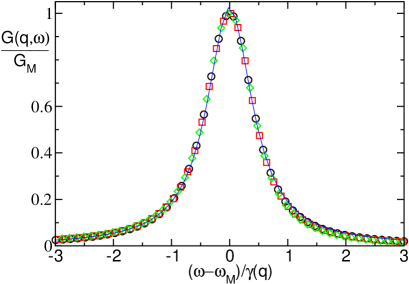
Figure 4: Quartic case: Fourier transform $G(q,\omega)$ of the correlation function for $\varepsilon=1$, $N=2000$ and the three wavenumbers $q=\pi/100$ (circles), $2\pi/100$ (squares), and $3\pi/100$ (diamonds). The solid line corresponds to the approximate analytical solution obtained by Fourier transforming the expression defined in (25,32).

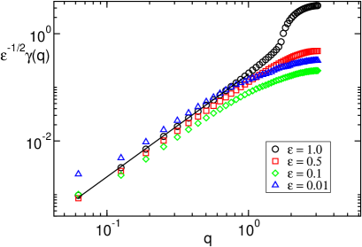
Figure 5: Scaling of the linewidth $\gamma(q)$ of $G(q,\omega)$ for four different values of the coupling constant $\varepsilon$ and $N=100$. The curves are obtained by integrating over $10^{4}$ time units. The solid line with slope 1.91 is a fit of the data corresponding to $\varepsilon=1$.

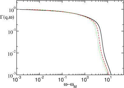
Figure 6: Fourier transforms of the memory function for three values of the wave-vector for $q=\pi/100$ (solid line), $2\pi/100$ (dashed line), and $3\pi/100$ (dotted line). For small frequencies they tend to a constant as we expect by analytic solution.

5 Energy current correlator

In the previous sections we have solved the mode-coupling equations as it applies to monoatomic chain of anharmonic oscillators for two distinct leading nonlinearities. Here, we use such results to determine the transport properties of the underlying lattice. In particular, we are interested in the thermal conductivity as defined by the Green-Kubo formula,

$$\kappa\;\propto\;\int_{0}^{\infty}\,\langle J(t)J(0)\rangle\,dt$$ (34)

where $J(t)$ is the total heat current, and $\langle\ldots\rangle$ brackets denote the equilibrium average. A general expression for the heat current has been derived in [11]. For the determination of the scaling behaviour it is sufficient to consider only the harmonic part, which can be expressed as a sum over wavevectors

$$J\;=\;\sum_{q}b(q)Q(q,t)P^{*}(q,t)$$ (35)

where $Q(q,t)$, and $P(q,t)=\dot{Q}(q,t)$ are the canonical variables in Fourier space and

$$b(q)=i\omega(q)\frac{\partial\omega(q)}{\partial q}\quad.$$ (36)

This amounts to disregarding higher-order terms which are believed not to modify the leading behaviour. Under the same approximations that allow deriving the mode-coupling equations, i.e. by neglecting correlations of order higher than two, one obtains,

$$\langle J(t)J(0)\rangle=\sum_{q}\mid b(q)\mid^{2}\{\langle Q(q,t)Q(q,0)\rangle\langle P(q,t)P^{*}(q,0)\rangle+\langle Q(q,t)P^{*}(q,0)\rangle^{2}\}$$ (37)

This expression can be further simplified under the assumption $P(q)\approx\omega(q)Q(q)$, that is certainly valid in the small $q$-limit. Altogether, this leads to the expression proposed in [17],

$$\langle J(t)J(0)\rangle\;\propto\;\sum_{q}\,\Big{(}\frac{d\omega(q)}{dq}\Big{)}^{2}G^{2}(q,t)$$ (38)

By taking into account the general expression (5), one obtains

$$\langle J(t)J(0)\rangle\;\propto\;\int dq\,\Big{[}C^{2}(q,t)e^{2iqt}+{C^{*}}^{2}(q,t)e^{-2iqt}+2C(q,t)C^{*}(q,t)\Big{]}$$ (39)

where, as usual in the thermodynamic limit, we have replaced the sum with an integral and have made use of the fact that for small $q$ (the integral is dominated by the small-$q$ terms), $\omega(q)\approx q$. We can finally use (11) to determine the scaling behaviour of the heat flux autocorrelation. Since the contribution of the terms proportional to ${\rm e}^{2iqt}$ is negligible, due its “rapid” oscillations, one obtains,

$$\langle J(t)J(0)\rangle\;\propto\;\int dq\,g^{2}(\sqrt{\varepsilon}tq^{3/2})\;\propto\;\frac{1}{t^{2/3}}$$ (40)

The resulting integral in equation (34) thereby diverges, revealing that the effective conductivity of an infinite lattice is infinite. In order to estimate the dependence of $\kappa$ on the system size $L$ it is customary to restrict the integration range to times smaller than $L/c$ where $c$ is the sound velocity. As a result, one finds that $\kappa(L)$ diverges as $L^{1/3}$, i.e. $\alpha=1/3$. Therefore we conclude that mode coupling predictions are now in full agreement with those of the renormalization group [12].

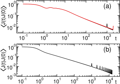
Figure 7: Correlation function of the heat-flux for the cubic (a) and quartic (b) case. The curves have been obtained for $N=2000$. In (a), also the outcome of a calculation made with $N=4000$ are plotted to show the good overlap in this time interval; the major difference is the obvious shift of the peak observed for a time equal to the system length divided by the sound velocity.

A similar analysis for the quartic case, leads, using equation (25), to

$$\langle J(t)J(0)\rangle\;\propto\;\int dq\,g^{2}(q^{2}t)\propto\frac{1}{t^{1/2}}$$ (41)

which, in turn, corrsponds to $\kappa\sim L^{1/2}$, i.e. $\alpha=1/2$. Finally, we have compared the theoretical predictions with the computation of the sum (38) complemented by direct integration of the mode coupling equations for $G(q,t)$ (see figure 7). A fit of the scaling region yields a slope equal to $-0.69$ in (a) and $-0.55$ in (b) to be compared with the theoretical expections that are respectively equal to $-2/3$ and $-1/2$. The deviations are analogous to those ones observed in the previous explicit analysis of the behaviour of $G(q,t)$ itself and can thus be attributed to finite size/time corrections.

6 Conclusions

In this paper we solved exactly the 1D MCT corresponding to a chain of nonlinear oscillators. The only assumption we made is that the dynamics of both the correlator $G(q,t)$ and the memory function $\Gamma(q,t)$ factorizes in the product of a “rapidly” oscillating term times a slowly decaying function, see equation (5). This Ansatz is confirmed a posteriori by the scaling of the analytic solution and by numerical calculations. The oscillating behaviour of $\Gamma(q,t)$ represents an element of novelty that was disregarded in previous studies [15, 17] (see hovever the perturbative calculation in [27]). In fact, taking the oscillations into account, we find that the decay of the envelope $M(q,t)$ depends on the order of the leading nonlinearity of the theory. In the cubic case, $M\propto t^{-2/3}$, while a faster decay, $M\propto t^{-1}$, is found in the quartic one, see equations (16,30). As a consequence, in the two cases, the decay of $G(q,t)$ is, respectively, anomalous (i.e. nonexponential) and exponential, see equations (18,32). Upon comparing with the solution of the Markovian equation (2), we thus argue that the cubic case is characterized by a diverging viscosity $\eta$, while a normal hydrodynamic behaviour (finite $\eta$) is found in the quartic case. At the same time, the other transport coefficient, the thermal conductivity $\kappa$, diverges in both cases. Indeed, the energy–current autocorrelation (as estimated from equation (38)) shows a long–time tail, $t^{-2/3}$ and $t^{-1/2}$ in the cubic an the quartic case, respectively. This implies that for large $L$, $\kappa$ diverges as $L^{\alpha}$, with $\alpha=1/3$ (cubic nonlinearity) or $\alpha=1/2$ (quartic nonlinearity).

Since generically, the leading nonlinear term is cubic, we can conclude that our analysis reconciles MCT with the renormalization-group prediction [12]. Accordingly, on the theoretical side there is no longer any doubt on the existence of a wide universality class characterized by the exponent $\alpha=1/3$.

The quartic case is less generic, since it requires the fine tuning of a control parameter (as for phase transitions) or the presence of a symmetry forbidding the existence of e.g. odd terms in the potential. This is, for instance, the case of the FPU-$\beta$ model which, by construction, contains only quadratic and quartic terms. In fact, the most accurate numerical findings obtained for the FPU-$\beta$ model [21] are qualitatively compatible with the scenario emerging from the analytic solution of the MCT in the quartic case, since $\alpha>2/5$ and does not exhibit a clear saturation with the system size.

The two-universality-class scenario emerging from our solution of the MCT is consistent with that one outlined in [31]. There, the scaling behavior has been estimated by complementing hydrodynamic and thermodynamic arguments under suitable assumptions. Such an analysis, that applies to quartic nonlinearity, predicts the same behavior for $\kappa$ as ours, as well as a finite $\eta$. As the Authors of reference [31] pointed out, the cubic case requires a fully self-consistent calculation which is precisely the task we accomplished here. Moreover, as already remarked, we conclude that both transport coefficients diverge. In addition, we argue that since $M$ and $\langle J(t)J(0)\rangle$ decay with the same power-law, $\eta$ should scale in the same way as $\kappa$. A few words are also needed to comment about the definition of the second class, which is identified in the present paper from the vanishing of the cubic term in the expansion of the effective potential (1), while in [31] from the equality between constant–pressure and constant–volume specific heats. At least in the FPU-$\beta$ model both constraints are simultaneously fulfilled. More in general, it seems plausible that these are two equivalent definitions of the same class but it is not certain.

Altogether, one of the important consequences of our analytical treatment is that fluctuations and response of 1D models cannot be accounted for by simple equations such as (2). Indeed, memory effects emerging from the nonlinear interaction of long-wavelength modes are essential and cannot be considered as small corrections. As a consequence, (2) should be replaced by equations like (20), meaning that hydrodynamic fluctuations must be described by generalized Langevin equation with power-law memory [32, 33]. This provides a sound basis for the connection between anomalous transport and kinetics (superdiffusion in this case) [34].

Finally, a few words on the consistency between this theoretical analysis and the simulation of specific models. Over the years it has become clear that numerical studies are affected by various types of finite-size corrections which make it difficult if not impossible to draw convincing conclusions (and this is one of the main reasons why we turned our attention to analytical arguments). The ubiquity of slow corrections suggests to carefully consider all the implicit assumptions made in the various theories, in the hope to understand the possibly universal origin of such deviation or even (though unlikely) to obtain corrections to the leading exponents. In this perspective, we wish to point out that the MCT solved in this paper is based on the assumption that the hydrodynamic properties are dominated by the coupling among sound-modes. A more general and complete mode-coupling analysis should consider also the coupling with thermal modes. General considerations indicate that the asymptotic scaling properties are not affected by lower-order corrections emerging in this more general approach. On the other hand, numerical experiments seem to suggest that such corrections could affect significantly finite size/time corrections to the scaling.

References

References

- [1] Pomeau Y and Résibois R, 1975 Phys. Rep. 63 19
- [2] Kirkpatrick TR, Belitz D and Sengers JV, 2002 J. Stat. Phys. 109, 373
- [3] Bishop M, 1982 J. Stat. Phys. 29 (3), 623
- [4] Lepri S, Sandri P, Politi A, 2005 Eur. Phys. J. B 47, 549
- [5] D’Humieres D, Lallemand P, Qian Y, 1989 C. R. Acad. Sci. Paris 308, serie II 585.
- [6] Hahn K, Kärger J, and Kukla V, 1996 Phys. Rev. Lett. 76, 2762
- [7] Morelli DT et al., 1986 Phys. Rev. Lett. 57, 869
- [8] Maruyama S, 2002 Physica B 323, 193; Mingo N and Broido DA, 2005 Nanoletters 5 1221
- [9] Lepri S, Livi R and Politi A, 1997 Phys. Rev. Lett. 78 1896
- [10] Lepri S, Livi R and Politi A, 1998 Europhys. Lett. 43, 271
- [11] Lepri S, Livi R and Politi A, 2003 Phys. Rep. 377 1
- [12] Narayan O and Ramaswamy S, 2002 Phys. Rev. Lett. 89 200601
- [13] Götze W in Liquids, freezing and the glass transition, edited by Hansen JP, Levesque D and Zinn-Justin J (North Holland, Amsterdam 1991); Schilling R in Collective dynamics of nonlinear and disordered systems, edited by Radons G, Just W and Häussler P (Springer, Berlin, 2003).
- [14] Ernst MH, 1991 Physica D 47, 198
- [15] Lepri S, 1998 Phys. Rev. E 58 7165
- [16] Pereverzev A, 2003 Phys. Rev. E 68, 056124
- [17] Wang J-S and Li B, 2004 Phys. Rev. Lett. 92 074302; 2004 Phys. Rev. E 70 021204
- [18] Lepri S, Livi R and Politi A, 2005 Chaos, 15 015118
- [19] Casati G, 1986 Found. Phys. 16 51; Hatano T, 1999 Phys. Rev. E 59, R1
- [20] Cipriani P, Denisov S and Politi A, 2005 Phys. Rev. Lett. 94, 244301
- [21] Lepri S, Livi R and Politi A, 2003 Phys. Rev. E 68 067102
- [22] Lippi A and Livi R, 2000 J. Stat. Phys. 100, 1147; Grassberger P and Yang L, unpublished [cond-mat/0204247]; Delfini L et al., 2005 J. Stat. Mech. P05006
- [23] Delfini L, Lepri S, Livi R and Politi A, 2006 Phys. Rev. E 73, 060201(R)
- [24] Kubo R, Toda M and Hashitsume N, Statistical Physics II; Springer Series in Solid State Sciences, Vol. 31, Springer, Berlin, 1991.
- [25] Scheipers J, Schirmacher W, 1997 Z. Phys. B 103, 547
- [26] Landau LD and Lifshitz EM, Theory of Elasticity, Pergamon Press, London, third edition, 1986.
- [27] Lepri S, 2000 Eur. Phys. J. B 18 441
- [28] Lovesey SW, Balcar E, 1994 J. Phys. Condens. Matter 6 1253
- [29] Metzler R and Klafter J, 2000 Phys. Rep. 339 1
- [30] Mainardi F, 1996 Chaos, Solitons and Fractals 7 1461
- [31] Lee-Dadswell GR, Nickel BG and Gray CG, 2005 Phys. Rev. E 72 031202
- [32] Wang KG and Tokuyama M, 1999 Physica A 265 341
- [33] Lutz E, 2001 Phys. Rev. E 64 051106
- [34] Denisov S, Klafter J and Urbakh, 2003 Phys. Rev. Lett. 91 194301