Electron transport in a one dimensional conductor with inelastic scattering by self-consistent reservoirs

Abstract

We present an extension of the work of D’Amato and Pastawski on electron transport in a one-dimensional conductor modeled by the tight binding lattice Hamiltonian and in which inelastic scattering is incorporated by connecting each site of the lattice to one-dimensional leads. This model incorporates Büttiker’s original idea of dephasing probes. Here we consider finite temperatures and study both electrical and heat transport across a chain with applied chemical potential and temperature gradients. Our approach involves quantum Langevin equations and nonequilibrium Green’s functions. In the linear response limit we are able to solve the model exactly and obtain expressions for various transport coefficients. Standard linear response relations are shown to be valid. We also explicitly compute the heat dissipation and show that for wires of length $N>>\ell$, where $\ell$ is a coherence length scale, dissipation takes place uniformly along the wire. For $N<<\ell$, when transport is ballistic, dissipation is mostly at the contacts. In the intermediate range between Ohmic and ballistic transport we find that the chemical potential profile is linear in the bulk with sharp jumps at the boundaries. These are explained using a simple model where the left and right moving electrons behave as persistent random walkers.

I Introduction

Inelastic scattering provides a mechanism for dissipation and decoherence in quantum systems. These effects are important in considering transport properties of mesoscopic systems. Experimental examples are numerous and include studies of transport in systems such as single walled carbon nanotubes Tans et al. (1997), atomic chains Ohnishi et al. (1998); Yanson et al. (1998), semiconducting heterostructures de Picciotto et al. (2001) and polymer nanofibers Zimbovskaya et al. (2005). In the absence of inelastic scattering, transport is either ballistic and we see effects such as conductance quantization van Wees et al. (1988); Wharam et al. (1988), or, with elastic scatterers we see effects of coherent scattering such as Anderson localization Gómez-Navarro et al. (2005). In either case transport is non-Ohmic even when we consider very long wires. Introducing inelastic scattering necessarily leads to decoherence and both of the above effects (ballistic transport, localization) are reduced. One expects that in the limit of long wires one should get Ohmic transport Datta (2005). Recent experiments on atomic chains Agraït et al. (2002) and Fullerene bridges Park et al. (2000); Pasupathy05 have studied the effects of inelastic scattering and the associated local heating on quantum transport.

The physical sources for inelastic scattering are well known and occur basically due to the interaction of the conducting electrons with other degrees of freedom in the system. For example these could arise due to electron-phonon interactions or interactions between conducting and non-conducting electrons Ziman (1972). However the microscopic modeling of inelastic scattering in the context of transport is nontrivial. One of the first phenomenological models for dissipation was due to Büttiker Büttiker (1985, 1986). In Büttiker’s model one connects a point inside the wire to a reservoir of electrons maintained at a chemical potential $\mu$ whose value is set by the condition that there is no average current flow into this side reservoir. This is equivalent to connecting a voltage probe at some point on the wire and a nice experimental realization of this situation can be seen in [de Picciotto et al., 2001]. In Büttiker’s model an electron flowing into the reservoir can emerge with a different phase and energy and thus one can have both decoherence and dissipation.

A more detailed microscopic calculation using Büttiker’s idea of incorporating inelastic scattering was performed by D’Amato and Pastawski D’amato and Pastawski (1990). In their study they considered transmission across a wire modeled by the tight-binding Hamiltonian with a nearest-neighbour hopping parameter $V$. Each site on the wire is connected to electron baths which are themselves modeled by tight-binding Hamiltonians with hopping parameter $\eta$. The wire is attached at the two ends to ideal leads with the same hopping parameter as the wire. These two leads are connected to reservoirs kept at fixed chemical potentials $\mu_{L}$ and $\mu_{R}$ for the left and right leads respectively. The side leads are attached to reservoirs whose chemical potentials are fixed self-consistently by imposing the condition of zero current. Using this model D’Amato and Pastawski analytically solved the case where the self-energy correction due to the side leads is pure imaginary and has the form $i\eta$ and $\eta$ is small. They were able to demonstrate the transition from coherent to Ohmic transport. An inelastic length scale $\ell=aV/\eta$, with $a$ as a lattice parameter, was introduced such that for wire length $L<<\ell$ transport was coherent while for $L>>\ell$ transport was Ohmic. A number of other papers Maschke and Schreiber (1991); Datta (1989); Datta and Lake (1991) have also shown that other models of inelastic scattering, for example due to electron-phonon (using side reservoirs as ensemble of harmonic oscillators to describe the heat bath) or electron-electron interactions, can be related to the Büttiker mechanism. Some recent papers have looked at electron-phonon interactions using the Keldysh nonequilibrium Green’s function formalism combined with density-functional methods Frederiksen et al. (2004), tight-binding molecular-dynamics Yamamoto et al. (2005) and the self-consistent Born approximation Asai (2004). An alternative mechanism for introducing inelastic scattering, through introduction of an imaginary potential in the Hamiltonian, has also been studied efetov95 ; mccann96 ; brouwer97 ; arun02 .

In the present paper we present an extension of the work of D’Amato and Pastawski. We study the case of transport of both heat and electron in the presence of inelastic scatterers in the form of self-consistent leads. The wire is subjected to both chemical potential and temperature gradients and we evaluate steady state values of both the particle and heat current operators. In the limit of a long wire when one is in the Ohmic regime we are able to obtain explicit expressions for all the linear response coefficients. It is verified that various linear response results such as Onsager reciprocity and the Weidemann-Franz law are valid. In the intermediate regime between ballistic and Ohmic transport we propose a simple model of right moving and left moving persistent random walkers which can explain much of the observed behaviour. We also perform an explicit calculation of the heat loss along the wire. This is a second order effect in the gradients and we show that there is uniform heat dissipation along the length of the wire whose value is precisely the Joule heat loss. For short wires we show that heat dissipation takes place primarily at the contacts. While heat dissipation by Büttiker probes has been discussed in [Büttiker, 1986; Lake and Datta, 1992], we believe that this is the first explicitly microscopic calculation of dissipation in a quantum wire that clearly demonstrates Joule heat loss in the Ohmic regime and dissipation into the reservoirs in the ballistic regime.

The formalism used in this paper is the quantum Langevin equations approach. In two recent papers Dhar and Sriram Shastry (2003); Dhar and Sen (2006) it was shown how this approach can be used to derive both the Landauer results and more generally the nonequilibrium Green’s function (NEGF) results on transport. Here we show how this method also works for the mulitple reservoir case and quickly leads to NEGF-like expressions for currents for both particle and heat. These equations are the starting point of our analysis. Thus apart from extending the results of [D’amato and Pastawski, 1990] we also use a different and more general approach. Unlike [D’amato and Pastawski, 1990] we also consider large values of the inelasticity parameter.

The paper is organized as follows. In sec. (II) we define the model and describe how the quantum Langevin approach can be used to get formal expressions for electron and heat currents in the steady state. In sec. (III) we write the self-consistent equations and discuss the linear response regime. In Sec. (IV) we solve the self-consistent equations for a long wire which is kept in a specified temperature gradient and evaluate the electical and heat current along the wire and also the heat loss into the side reservoirs. The transition from the ballistic to the Ohmic regime is briefly discussed in sec. (V). Finally we conclude with a discussion in sec. (VI).

II Model and general results

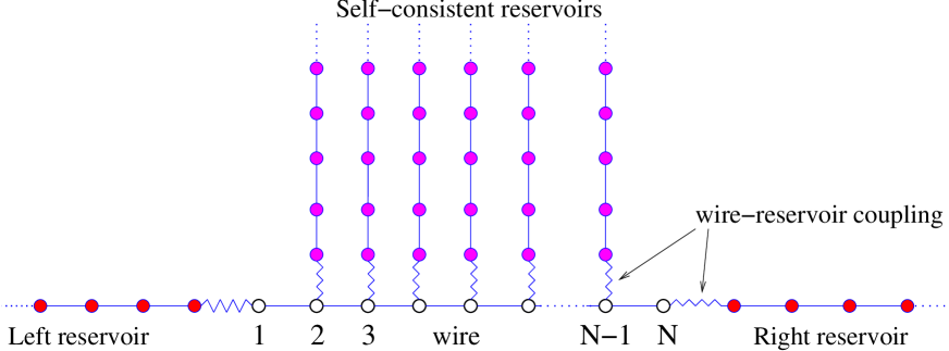
Figure 1: A schematic description of the model.

We consider a one-dimensional wire modeled by the tight-binding lattice Hamiltonian. The wire has $N$ sites each of which is coupled to an infinite reservoir which is itself modeled by a one-dimensional tight-binding system [see Fig. (1)]. The Hamiltonian of the system consisting of the wire and all the reservoirs is given by

$$\mathcal{H} = \mathcal{H}_{W}+\sum_{l=1}^{N}\mathcal{H}_{R}^{l}+\sum_{l=1}^{N}\mathcal{V}_{WR}^{l}$$

$${\rm where}~{}~{}~{}\mathcal{H}_{W} = -\sum_{l=1}^{N-1}\gamma~{}(c^{{\dagger}}_{l}c_{l+1}+c^{{\dagger}}_{l+1}c_{l})$$

$$\mathcal{H}_{R}^{l} = -\gamma_{l}~{}\sum_{\alpha=1}^{\infty}~{}(c^{l{\dagger}}_{\alpha}c^{l}_{\alpha+1}+c^{l{\dagger}}_{\alpha+1}c^{l}_{\alpha})~{}~{}~{}~{}l=1,2..N$$

$$\mathcal{V}_{WR}^{l} = -\gamma^{\prime}_{l}~{}(c^{l{\dagger}}_{1}c_{l}+c^{{\dagger}}_{l}c^{l}_{1})~{}~{}~{}~{}l=1,2...N~{}.$$ (1)

Here $c_{l}$ and $c_{\alpha}^{l}$ denote respectively operators on the wire and on the $l^{th}$ reservoir. The Hamiltonian of wire is denoted by $\mathcal{H}_{W}$, that of the $l^{\rm th}$ reservoir by $\mathcal{H}^{l}_{R}$ and the coupling between the wire and the $l^{\rm th}$ site is $\mathcal{V}^{l}_{WR}$. The coupling between the reservoirs and the wire is controlled by the parameters $\gamma^{\prime}_{l}$.

We briefly indicate the steps leading to generalized quantum Langevin equations of motion for the wire variables. We assume that for $t\leq t_{0}$ the reservoirs are disconnected from the wire. Each reservoir is in equilibrium at a specified temperature $T_{l}$ and chemical potential $\mu_{l}$. At time $t_{0}$ we connect all the reservoirs to the wire and we are interested in the steady state properties of the wire. For $t>t_{0}$, the Heisenberg equations of motion for the wire and reservoirs variables are:

$$\dot{c}_{l} = \frac{i\gamma}{\hbar}(c_{l-1}+c_{l+1})+\frac{i\gamma_{l}^{\prime}}{\hbar}c^{l}_{1}~{}~{}~{}~{}{\rm for}~{}~{}l=1,2...N~{},$$ (2)

$$\dot{c}^{l}_{\alpha} = \frac{i\gamma_{l}}{\hbar}({c^{l}}_{\alpha-1}+{c^{l}}_{\alpha+1})~{}~{}~{}~{}{\rm for}~{}~{}~{}\alpha=2,3,...\infty~{},~{}~{}l=1,2,...N$$ (3)

$$\dot{c}^{l}_{1} = \frac{i\gamma_{l}}{\hbar}c^{l}_{2}+\frac{i\gamma^{\prime}_{l}}{\hbar}c_{l}~{}~{}~{}{\rm for}~{}~{}l=1,2...N$$ (4)

and we have taken $c_{0}=c_{N+1}=0$. The equation of motion of the wire variables Eq. (2) involves the reservoir variable $c^{l}_{1}$ and we will try to eliminate this. We note that the equation of motion of each of the $N$ reservoirs, given by Eq. (3,4), is a set of linear equations with an inhomogeneous part given by $i\gamma^{\prime}_{l}c_{l}/\hbar$ . We can solve these equations of motion using the single particle Green’s function of the reservoirs which is given by $g^{l}(t)=-i\theta(t)e^{-iH^{l}t/\hbar}$ where $H^{l}$ is the single-particle Hamiltonian of the $l^{\rm th}$ reservoir and $\theta(t)$ the Heaviside step function. We finally find that the solution for the boundary site on the $l^{\rm th}$ reservoir is given by (for $t>t_{0}$)

$$c^{l}_{1}(t)=i\sum_{\alpha=1}^{\infty}g^{l+}_{1\alpha}(t-t_{0})c^{l}_{\alpha}(t_{0})-\int_{t_{0}}^{\infty}~{}dt^{\prime}~{}g^{l+}_{1,1}(t-t^{\prime})~{}\frac{\gamma^{\prime}_{l}}{\hbar}~{}c_{l}(t^{\prime})$$ (5)

Plugging this into the equation of motion Eq. (2) of wire variables, we get

$$\dot{c}_{l}(t) = \frac{i\gamma}{\hbar}(c_{l-1}+c_{l+1})-i\eta_{l}-i\int_{t_{0}}^{\infty}dt^{\prime}\Sigma^{+}_{l}(t-t^{\prime})c_{l}(t^{\prime})$$ (6)

$${\rm where}~{}~{}~{}\eta_{l}(t) = -\frac{i\gamma_{l}^{\prime}}{\hbar}~{}\sum_{\alpha=1}^{\infty}g^{l+}_{1\alpha}(t-t_{0})~{}c^{l}_{\alpha}(t_{0})$$

$$\Sigma^{+}_{l}(t) = (\frac{\gamma_{l}^{\prime}}{\hbar})^{2}~{}g^{l+}_{1,1}(t)$$

This is in the form of a generalised quantum Langevin equation where we identify $\eta_{l}$ as noise from the $l^{\rm th}$ reservoir and the last term in Eq. (6) is the dissipative term. The noise depends on the reservoir’s initial distribution which we have chosen to be an equilibrium distribution. The properties of the noise is written most conveniently in the frequency domain. We consider the limit $t_{0}\to-\infty$. Let us define the Fourier transforms $\tilde{c}_{l}(\omega)=(1/2\pi)\int_{-\infty}^{\infty}dte^{i\omega t}c_{l}(t)$, $g^{l+}(\omega)=\int_{-\infty}^{\infty}dte^{i\omega t}g^{l+}(t)$, $\tilde{\eta}_{l}(\omega)=(1/2\pi)~{}\int_{-\infty}^{\infty}dte^{i\omega t}\eta_{l}(t)$ and $\Sigma^{+}_{l}(\omega)=(\gamma^{\prime}_{l}/\hbar)^{2}g^{l+}_{1,1}(\omega)$. Let us also use the definition $\Gamma_{l}(\omega)=-Im[\Sigma^{+}_{l}]/\pi=(\gamma^{\prime}_{l}/\hbar)^{2}\rho_{l}(\omega)$ where $\rho_{l}(\omega)$ is the local density of states at the first site ($\alpha=1$) on the $l^{\rm th}$ reservoir. With these definitions it is easy Dhar and Sen (2006) to show that the noise-noise correlations are given by

$$\langle\tilde{\eta}_{l}^{\dagger}(\omega)\tilde{\eta}_{m}(\omega^{\prime})\rangle=\Gamma_{l}(\omega)~{}f(\omega,~{}\mu_{l},~{}T_{l})~{}\delta(\omega-\omega^{\prime})~{}\delta_{lm}~{},$$ (7)

where $f(\omega,\mu,T)=1/\{exp[(\hbar\omega-\mu)/k_{B}T]+1\}$ is the Fermi distribution function.

Taking Fourier transform of the equation of motion Eq. (6) we thus get the following steady state solution

$$\tilde{c}_{l}(\omega) = \sum_{m=1}^{N}~{}G^{+}_{lm}(\omega)~{}\tilde{\eta}_{m}(\omega)$$ (8)

$${\rm where}~{}~{}~{}G^{+} = \frac{\hbar}{\gamma}Z^{-1}$$

$${\rm and}~{}~{}~{}Z_{lm} = \frac{\hbar}{\gamma}(\omega-\Sigma^{+}_{l})~{}\delta_{lm}+\delta_{l,m-1}+\delta_{l,m+1}~{}.$$

As shown in [Dhar and Sen, 2006] $G^{+}(\omega)$ is basically the Green’s function of the full system (wire and reservoirs) and for points on the wire can be written in the form $G^{+}(\omega)=[\omega-H_{W}/\hbar-\bar{\Sigma}^{+}]^{-1}$ where $H_{W}$ is the single particle Hamiltonian of the wire while $\bar{\Sigma}^{+}$, defined by its matrix elements $\bar{\Sigma}^{+}_{lm}=\Sigma^{+}_{l}\delta_{lm}$, is a self-energy correction arising from the interaction with the reservoirs. We will be interested in particle and energy currents in the system. The corresponding operators are obtained by defining particle and energy density operators and obtaining their continuity equations Dhar and Sriram Shastry (2003). The particle density is defined on sites while the energy density is defined on bonds. We will be interested in currents both inside the wire and between the wire and reservoirs. Let us define $j^{p}_{l}$ as the particle current between sites $l~{},l+1$ on the wire and $j^{u}_{l}$ as the energy current between the bonds $(l-1,l)$ and $(l,l+1)$. Also we define $j^{p}_{w-l}$ as the particle current from the wire to the $l^{\rm th}$ reservoir and similarly $j^{u}_{w-l}$ is the energy current from the wire to the $l^{\rm th}$ reservoir. These are given by the following expectation values:

$$j^{p}_{l} = \frac{i\gamma}{\hbar}\langle~{}c_{l+1}^{\dagger}c_{l}-c_{l}^{\dagger}c_{l+1}~{}\rangle$$

$$j^{u}_{l} = \frac{i\gamma^{2}}{\hbar}\langle~{}c_{l-1}^{\dagger}c_{l+1}-c_{l+1}^{\dagger}c_{l-1}~{}\rangle$$

$$j^{p}_{w-l} = \frac{-i\gamma_{l}^{\prime}}{\hbar}\langle~{}c_{l}^{\dagger}c_{1}^{l}-{c_{1}^{l}}^{{\dagger}}c_{l}~{}\rangle$$

$$j^{u}_{w-l} = \frac{i\gamma\gamma_{l}^{\prime}}{\hbar}\langle~{}(c_{l+1}^{\dagger}+c_{l-1}^{\dagger})~{}c_{1}^{l}-{c^{l}_{1}}^{{\dagger}}(c_{l+1}+c_{l-1})~{}\rangle~{}.$$

Using the general solution in Eq. (8) and the noise properties in Eq. (7) we can evaluate the above expressions and find

$$j^{p}_{l} = \sum_{m=1}^{N}\frac{-i\gamma{\gamma^{\prime}_{m}}^{2}}{\hbar^{3}}\int_{-\infty}^{\infty}d\omega(~{}G^{+}_{lm}G^{-}_{ml+1}-G^{+}_{l+1m}G^{-}_{ml}~{})~{}\rho_{m}~{}(f_{l}-f_{m})$$ (9)

$$j^{u}_{l} = \sum_{m=1}^{N}\frac{i\gamma^{2}{\gamma^{\prime}_{m}}^{2}}{\hbar^{3}}\int_{-\infty}^{\infty}d\omega(~{}G^{+}_{l-1m}G^{-}_{ml+1}-G^{+}_{l+1m}G^{-}_{ml-1}~{})~{}\rho_{m}~{}(f_{l}-f_{m})$$ (10)

$$j^{p}_{w-l} = \sum_{m=1}^{N}\frac{1}{2\pi}\int_{-\infty}^{\infty}d\omega\mathcal{T}_{lm}~{}(f_{l}-f_{m})$$ (11)

$$j^{u}_{w-l} = \sum_{m=1}^{N}\frac{1}{2\pi}\int_{-\infty}^{\infty}d\omega~{}\hbar\omega~{}\mathcal{T}_{lm}~{}(f_{l}-f_{m})~{},$$ (12)

where $G^{-}_{lm}={G^{+}_{ml}}^{*}$ and $\mathcal{T}_{lm}=4\pi^{2}{\gamma^{\prime}_{l}}^{2}{\gamma^{\prime}_{m}}^{2}\rho_{l}\rho_{m}|G_{lm}^{+}|^{2}/\hbar^{4}$ can be shown to be the transmission probability of a wave from the $l^{\rm th}$ to the $m^{\rm th}$ reservoir.

III Self-consistent determination of chemical potential profile

We consider the case where the wire is held in a fixed temperature field specified by the temperatures, $T_{l},~{}l=1,2...N$, of the $N$ reservoirs. We will consider a small temperature difference and assume that the applied temperature field has the linear form

$$T_{l}=T_{L}+\frac{l-1}{N-1}\Delta T~{},$$

where $\Delta T=T_{R}-T_{L}$. The chemical potentials at the ends of the wire are specified by the conditions $\mu_{1}=\mu_{L}$ and $\mu_{N}=\mu_{R}$. The $N-2$ side reservoirs $l=2,3...N-1$ are included to simulate other degrees of freedom present in a real wire and the requirement of zero net particle current into these reservoirs self-consistently fixes the values of their chemical potentials. Thus the chemical potentials $\{\mu_{l}\}$ for $l=2,3...N-1$ are obtained by solving the following set of $N-2$ equations:

$$j^{p}_{w-l}=0~{}~{}~{}{\rm for}~{}~{}~{}l=2,3,...N-1~{},$$ (13)

with $j^{p}_{w-l}$ given by Eq. (11). Once the chemical potential profile is determined, we can use Eqs. (9,10) to determine the particle and heat currents in the system while Eq. (12) gives the heat exchange with the environment (side reservoirs).

In general the set of equations Eq. (13) are nonlinear and difficult to solve analytically. We will henceforth consider the low temperature and linear response regime where the applied chemical potential difference $\Delta\mu=\mu_{R}-\mu_{L}$ and the temperature difference $\Delta T$ are both small. More specifically we shall assume $\Delta\mu<<\mu_{L,R},~{}\Delta T<<T_{L,R}$ and $k_{B}T_{L,R}<<\mu_{L,R}$. For simplicity we restrict ourselves to the following choice of parameters: $\gamma_{l}=\gamma^{\prime}_{1}=\gamma^{\prime}_{N}=\gamma$ for $l=1,2...N$ and $\gamma^{\prime}_{l}=\gamma^{\prime}$ for $l=2,3...N-1$. Thus all the reservoirs will have the same Green’s function and density of states and we will use the notation $g^{l+}_{1,1}(\omega)=g^{+}(\omega)$ and $\rho_{l}(\omega)=\rho(\omega)$.

Making Taylor expansions of the Fermi functions $f(\omega,\mu_{l},T_{l})$ about the mean values $\mu=(\mu_{L}+\mu_{R})/2$ and $T=(T_{L}+T_{R})/2$, we find that, in the linear response regime, Eq. (13) reduces to the following set of equations:

$$j^{p}_{w-l}=\sum_{m=1}^{N}\frac{1}{2\pi\hbar}~{}[~{}\mathcal{T}_{lm}~{}(\mu_{l}-\mu_{m})+\frac{\pi^{2}k_{B}^{2}T}{3\hbar}~{}\mathcal{T}^{\prime}_{lm}(T_{l}-T_{m})~{}]=0~{}~{}~{}{\rm for}~{}~{}~{}l=2,3...N-1~{},$$ (14)

where $\mathcal{T}_{lm}$ and $\mathcal{T}^{\prime}_{lm}=d\mathcal{T}_{lm}/d\omega$ are evaluated at $\omega=\mu/\hbar$. These are linear equations in $\{\mu_{l}\}$ and are straightforward to solve numerically. We can then use Eq. (9) and Eq. (10) to find the particle and heat current. The local heat current in the wire is given by $j^{q}_{l}=j^{u}_{l}-\mu_{l}j^{p}_{l}$. In the linear response regime we find

$$j^{p}_{l} = \frac{-1}{2\pi\hbar}\sum_{m=1}^{N}[\mathcal{F}_{lm}~{}(\mu_{l}-\mu_{m})+\frac{\pi^{2}k_{B}^{2}T}{3\hbar}\mathcal{F}^{\prime}_{lm}~{}(T_{l}-T_{m})]$$

$$j^{q}_{l} = \frac{-1}{2\pi\hbar}\sum_{m=1}^{N}[~{}\frac{\pi^{2}k_{B}^{2}T^{2}}{3\hbar}\mathcal{F}^{\prime}_{lm}~{}(\mu_{l}-\mu_{m})+\frac{\pi^{2}k_{B}^{2}T}{3}\mathcal{F}_{lm}~{}(T_{l}-T_{m})~{}]~{},$$ (15)

where $\mathcal{F}_{lm}=(2\pi i\gamma\gamma^{\prime 2}/\hbar^{3})~{}(~{}G^{+}_{lm}G^{-}_{ml+1}-G^{+}_{l+1m}G^{-}_{ml}~{})~{}\rho$ and $\mathcal{F}_{lm},\mathcal{F}^{\prime}_{lm}$ are evaluated at $\omega=\mu/\hbar$. The heat loss from the wire to the reservoir can be obtained using Eq. (12). As we shall see later this heat loss is a second order effect and therefore we will keep terms up to second order in the expansion. We then get

$$j^{q}_{w-l}=\frac{1}{2\pi\hbar}\sum_{m=1}^{N}\left[-\frac{\pi^{2}k_{B}^{2}T^{2}}{3\hbar}\mathcal{T}^{\prime}_{lm}~{}(\mu_{l}-\mu_{m})-\frac{\pi^{2}k_{B}^{2}T}{3}\mathcal{T}_{lm}~{}(T_{l}-T_{m})~{}\right.$$ (16)

$$+ \left.\frac{1}{2}\mathcal{T}_{lm}~{}(\mu_{l}-\mu_{m})^{2}+\frac{2\pi^{2}k_{B}^{2}T}{3\hbar}~{}\mathcal{T}^{\prime}_{lm}~{}(\mu_{l}-\mu_{m})(T_{l}-T_{m})+\frac{\pi^{2}k_{B}^{2}}{3}~{}\mathcal{T}_{lm}~{}(T_{l}-T_{m})^{2}~{}\right].$$

In the next section we will the consider the case of a long wire ($N\to\infty$) and consider particle and heat transport in the presence of applied chemical potential and temperature gradients. Later, for an isothermal system, we will consider finite systems and discuss the transition from coherent to Ohmic transport.

IV Long wire with applied chemical potential and temperature gradients

Let us first evaluate the matrix elements $\mathcal{T}_{lm}(\omega)$. This involves $\rho(\omega)$ and $G^{+}_{lm}(\omega)$. As discussed before $\rho(\omega)$ is the local density of states at the boundary site of a semi-infinite one-dimensional chain and is given by $\rho(\omega)=({\hbar}/{(\pi\gamma)}[1-{\hbar^{2}\omega^{2}}/{(4\gamma^{2})}]^{1/2}$ for $|\hbar\omega|<2\gamma$ and zero elsewhere. For lattice points in the bulk of the wire, i.e points which are at a distance $>>\ell=1/\alpha_{R}$ from the boundaries of the wire we find (see Appendix A) $G^{+}_{lm}={(-1)^{l+m}\hbar~{}e^{-|l-m|\alpha}}/(2\gamma\sinh{\alpha})$. We now try the following solution for the self-consistent equations given by Eq. (14):

$$\mu_{l}=\mu_{L}+\frac{l-1}{N-1}\Delta\mu~{}.$$ (17)

Using the fact that $\sum_{m=-\infty}^{m=\infty}(l-m)~{}e^{-|l-m|\alpha}=0$, we see that the self-consistent equations are satisfied for all points $l$ in the bulk of the wire (up to corrections which become exponentially small with the distance from the boundaries). Close to the boundaries the chemical potential variation is no longer linear. Here we focus on the limit where $N$ is very large and the linear solution in Eq. (17) is accurate in the bulk of the wire.

We will now use this solution to evaluate the various currents in the wire given by Eq. (15) and the heat loss from Eq. (16). We evaluate these currents at points $l$ in the bulk of the wire and (since $G^{+}_{lm}$ decays exponentially with distance) do not need the correct form of $\mu_{l}$ at the boundaries. We also find, as expected, that the currents are independent of $l$. They have the expected linear response forms:

$$j^{p} = -L_{11}\nabla\mu-L_{12}\nabla T$$

$$j^{q} = -L_{21}\nabla\mu-L_{22}\nabla T~{},$$

where $\nabla\mu=\Delta\mu/N$, $\nabla T=\Delta T/N$ and the various transport coeficients are given by

$$L_{11} = \frac{1}{2\pi\hbar}\sum_{m=-\infty}^{\infty}\mathcal{F}_{lm}(\mu/\hbar)~{}(l-m)=\frac{1}{\pi\hbar}~{}\frac{\sin^{2}{\alpha_{I}}\coth{\alpha_{R}}}{\cosh 2{\alpha_{R}}-\cos 2{\alpha_{I}}}~{},$$ (18)

$$L_{12} = \frac{\pi^{2}k_{B}^{2}T}{3}~{}\frac{dL_{11}}{d\mu}~{},$$ (19)

$$L_{21} = T~{}L_{12}~{},$$ (20)

$$L_{22} = \frac{{\pi}^{2}k_{B}^{2}T}{3}~{}L_{11}~{},$$ (21)

where $\alpha_{R}$ and $\alpha_{I}$ are respectively the real and imaginary parts of $\alpha$ and are all calculated at $\omega=\mu/\hbar$. In deriving the above form of $L_{11}$ we have used the relation $\rho=2\gamma\hbar\sinh{\alpha_{R}}\sin{\alpha_{I}}/(\pi{\gamma^{\prime}}^{2})$. In the parameter regime we are looking at, it follows that both Ohm’s law and Fourier’s law are valid, with the electrical and thermal conductivities given by $\sigma=e^{2}L_{11}$ and $\kappa=L_{22}$. We note that Eq. (20) gives the Onsager reciprocity relation. This is usually derived within linear response theory and follows from time reversal invariance of the microscopic equations of motion. We also find from Eq. (21) that the Weidemann-Franz relation is satisfied. This relation states that the ratio of the thermal conductivity and the electrical conductivity is linearly proportional to the temperature with a universal constant of proportionality given by ${\pi^{2}k_{B}^{2}}/{(3e^{2})}$. For metals a derivation of this relation using semiclassical tramsport theory and within the relaxation time approximation can be found in [ashcroft, ]. The validity of this relation requires that inelastic processes can be neglected ( see discussion in [ashcroft, ] ). However we find that the relation continues to be valid in our model even though scattering is inelastic (since there is energy dissipation into the side reservoirs).

From Eq (19) we find that the Mott formula for the thermopower holds mott ; lunde05 . This is given by

$$Q=\frac{L_{12}}{eL_{11}}=\frac{\pi^{2}k_{B}^{2}T}{3e}\frac{1}{\sigma}\frac{d\sigma}{d\mu}~{}.$$ (22)

Recently [lunde06, ] have reported an interesting resonance, arising due to electron-electron interactions, observed in the thermopower as a function of the Fermi energy. We investigate if there are any interesting features in the dependence of $Q$ on $\mu$ in our model. In Fig (2) we plot the conductivity and the thermopower $3eQ/(\pi^{2}k_{B}^{2}T)=d(\ln\sigma)/d\mu$ as a function of $\mu$ for different values of the coupling constant $\gamma^{\prime}$. Surprisingly we find that for a range of values of the inelasticity parameter $\gamma^{\prime}$ there is a peak in the thermopower as a function of the Fermi energy.

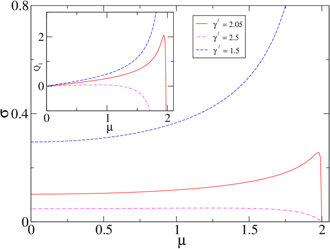
Figure 2: Plot of the conductivity and thermopower $Q_{1}=3eQ/(\pi^{2}k_{B}^{2}T)$ (Inset) as functions of the Fermi level $\mu$ for different values of the inelasticity parameter $\gamma^{\prime}$. They are plotted in units of $e^{2}/\pi\hbar$ and $\gamma$ respectively.

Let us now look at the heat exchanges given by Eq. (16). In the long-wire limit, the condition of zero particle currents into the side reservoirs, Eq. (14), implies that $\sum_{m}\mathcal{T}_{lm}(l-m)=\sum_{m}\mathcal{T}^{\prime}(l-m)=0$. Hence the terms linear in $\nabla\mu$ and $\nabla T$ in Eq. (16) vanish, and only the second order terms contribute significantly. Let us first consider the coefficient of the term containing $(\nabla\mu)^{2}$ which is given by

$$\frac{1}{4\pi\hbar}\sum\mathcal{T}_{lm}~{}(l-m)^{2}~{}.$$ (23)

Evaluating the sum we find that it is exactly equal to $L_{11}$. Determining the other terms in Eq. (16) we find that the net heat loss per unit length (or from every bulk site) of the wire is given by:

$$j^{q}=L_{11}~{}(\nabla\mu)^{2}+\frac{4\pi^{2}k_{B}^{2}T}{3}~{}\frac{dL_{11}}{d\mu}~{}(\nabla\mu)(\nabla T)+\frac{2\pi^{2}k_{B}^{2}}{3}~{}L_{11}(\nabla T)^{2}~{}.$$ (24)

The first term corresponds to the expected Joule heat loss in a wire and is always positive. The second term can be of either sign and can be identified to be the Thomson effect which corresponds to heat exchange that occurs in a wire (in addition to the Joule heat) when an electric current flows across a temperature gradient.

Finally we check for local thermal equilibrium in the wire. A requirement of local equilibrium would be that the local density $n_{l}$ at the point $l$ in the nonequilibrium state should be the same as the density $n^{eq}_{l}$ at the point if the entire wire was kept in equilibrium at a chemical potential $\mu_{l}$ and temperature $T_{l}$. It is easy to evaluate $n_{l}$ and $n^{eq}_{l}$ and we find:

$$n_{l}-n^{eq}_{l}=\sum_{m=1}^{N}\frac{{\gamma^{\prime}}^{2}}{\hbar^{2}}\int_{-\infty}^{\infty}d\omega|G^{+}_{lm}(\omega)|^{2}~{}\rho(\omega)~{}[~{}f(\omega,\mu_{m},T_{m})-f(\omega,\mu_{l},T_{l})~{}]~{},$$

which in the linear response regime, gives

$$n_{l}-n^{eq}_{l}=\frac{{\gamma^{\prime}}^{2}}{\hbar^{3}}~{}\sum_{m=1}^{N}\left[~{}|G^{+}_{lm}(\mu/\hbar)|^{2}~{}\rho(\mu/\hbar)~{}(\mu_{l}-\mu_{m})+\frac{\pi^{2}k_{B}^{2}T}{3}~{}\frac{d}{d\mu}[|G^{+}_{lm}(\mu/\hbar)|^{2}\rho(\mu/\hbar)]~{}(T_{l}-T_{m})~{}\right]~{}.$$

For our linear profiles of temperature and chemical potential and the form of $G_{lm}$ it is clear that, for all bulk points, the above difference vanishes (upto order $O(1/N)$). Thus we see that the local densities are consistent with the assumption of local equilibrium.

V Current flow in wire in isothermal conditions: finite size effects

In this section we look at finite length wires. We first solve Eq. (14) numerically to determine the chemical potential profile and then estimate the current in the wire using Eq. (15). We also look at the local heat dissipation at all points on the wire.

In our numerical calculations we have chosen the parameter values $\mu_{L}=1.0,\mu_{R}=1.1,\gamma=1.0$ and have considered different values of the dissipation strength $\gamma^{\prime}$ and different system sizes $N$. In Fig. (3) we plot the chemical potential profile, for different system sizes, for a small value of the dissipation ($\gamma^{\prime}=0.1$). We see that as we go to larger system sizes, chemical potential profile changes, from a flat profile with large jumps at the boundaries, to a smooth linear profile. For a larger dissipation parameter ($\gamma^{\prime}=1.0$) we see [inset of Fig. (3)] that a smooth linear profile is obtained even for small system sizes.

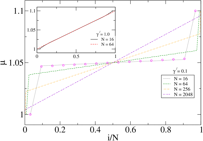
Figure 3: Plot of the chemical potential profile $\mu_{i}$ as a function of the scaled length $i/N$ for different values of $N$ and with $\gamma^{\prime}=0.1$. The points denoted by circles correspond to the approximate solution given in Eq. (26). The inset shows the chemical potential profile for $\gamma^{\prime}=1.0$.

The limit of weak dissipation was studied in [D’amato and Pastawski, 1990] . Following them we find that for $\gamma^{\prime}/\gamma<<1$ a very good approximation for the transmission coefficients $\mathcal{T}_{lm}$, for any system size, is given by

$$\mathcal{T}^{+}_{lm}=\frac{\pi^{2}{\gamma^{\prime}_{l}}^{2}{\gamma^{\prime}_{m}}^{2}\rho^{2}}{{\hbar}^{2}\gamma^{2}}e^{-\frac{2|l-m|}{\ell}}~{}.$$ (25)

where $\ell=1/\alpha_{R}\approx 2\gamma^{2}/\gamma^{\prime 2}$. Note that, for $l=2,3,...N-1$, $\mathcal{T}_{1l}$ and $\mathcal{T}_{lN}$ are $O({\gamma^{\prime}}^{2})$ while $\mathcal{T}_{lm}$ for $m=2,3,...N-1$ are $O({\gamma^{\prime}}^{4})$. We then find that, for $\ell>>1$ and $N>>1$, the following chemical potential profile provides a good approximate solution of the self-consistent equations:

$$\mu_{1} = \mu_{L},~{}~{}\mu_{N}=\mu_{R}$$

$$\mu_{l} = \mu_{L}-\delta-\frac{2\delta}{\ell}(l-2)~{}~{}~{}{\rm for}~{}~{}l=2,3,...N-1$$ (26)

$${\rm where}~{}~{}~{}\delta = \frac{\mu_{L}-\mu_{R}}{2(1+N/\ell)}$$

Plugging in this solution into the self-consistency equations $\sum_{m}\mathcal{T}_{lm}(\mu_{l}-\mu_{m})=0$ with $\mathcal{T}_{lm}$ given by Eq. (25) we can explicitly verify that these are satisfied upto corrections of order $1/\ell$. In Fig. (3) we have plotted the above solution for system size $N=16$ and find an excellent agreement with the numerical result (for larger system sizes the fit agreement becomes better).

The above solution leads to the following result for the current:

$$\frac{jN}{\Delta\mu L_{11}}=\frac{1}{1+\ell/N}~{},$$ (27)

where $L_{11}$ is the ohmic conductivity of the wire given by Eq. (18) and we have normalized the current such that the $N\to\infty$ limit gives a constant value independent of $\gamma^{\prime}$.

We have also looked at the transition from coherent to Ohmic transport for general values of the dissipation parameter $\gamma^{\prime}$. In Fig. (4) we plot the scaled current $jN/(\Delta\mu L_{11})$ as a function of system size. We find that in general for any $\gamma^{\prime}/\gamma<1$ the data can be fitted quite accurately to the form in Eq. (27) with $\ell=1/\alpha_{R}$ which can be interpreted as a coherent length scale. For $\gamma^{\prime}/\gamma>1$ we find that there is no coherent regime and the approach to the asymptotic limit has a different form.

Persistent random walk model: It is possible to understand the various aspects of the intermediate regime within a simple classical Drude-like framework of right moving and left moving electrons moving in fixed directions but with a small probability of inter-conversion. We consider the case where the left reservoir is kept at a chemical potential $\mu+\Delta\mu$ and the right reservoir is at $\mu$. At the low temperatures being considered electron transport is basically due to the electrons close to the Fermi level and we can focus on the electrons within the energy gap $\Delta\mu$ in the left reservoir. Let the density of these electrons inside the left reservoir be $2\rho_{L}$ and this consists of an equal proportion of right moving electrons with velocity $v_{F}$ and left movers with velocity $-v_{F}$. In the right reservoir the density of both left and right movers in the energy window $\Delta\mu$ is zero. Inside the wire the presence of the side-reservoirs allows a right mover to be converted to a left mover with some probability. We now present the following random walk model to incorporate the above basic idea. The model consists of a lattice of $N$ sites with a density $\rho_{l}^{+}$ of right movers and $\rho_{l}^{-}$ of left movers at all sites $l=1,2...N$. We impose the boundary conditions $\rho_{1}^{+}=\rho_{1}^{-}=\rho_{L}$ and $\rho_{N}^{+}=\rho_{N}^{-}=0$. At sites $l=2,3...N-1$ the particles move according to the following rules: with probability $p$ a right mover at site $l$ moves to $l+1$ and, with probability $1-p$ it transforms to a left mover and moves to site $l-1$. Similarly, with probability $p$ a left mover at site $l$ moves to $l-1$ and, with probability $1-p$ it transforms to a right mover and moves to $l+1$. At sites $l=1,N$, the right mover always moves to the right and the left mover moves to the left. It is then straightforward to write discrete time-evolution equations for the density fields $\rho_{i}^{+}(t)$ and $\rho_{i}^{-}(t)$. Choosing a lattice length scale $a$ and a microscopic time scale $\tau$ we obtain, in the continuum limit

$$\frac{\partial\rho^{+}(x,t)}{\partial t} = -v\frac{\partial\rho^{+}}{\partial x}-\alpha(\rho^{+}-\rho^{-})$$

$$\frac{\partial\rho^{-}(x,t)}{\partial t} = v\frac{\partial\rho^{-}}{\partial x}+\alpha(\rho^{+}-\rho^{-})~{}.$$ (28)

where $v=ap/\tau$ can be identified with the Fermi velocity $v_{F}$ and $\alpha=(1-p)/\tau$ gives the scattering rate (Note that the continuum limit requires taking $a\to 0$, $\tau\to 0$ and $p\to 1$ keeping $v$ and $\alpha$ finite). We obtain a length scale $v/\alpha$ which we tentatively identify with the scattering length $\ell$ introduced earlier. The boundary conditions for the above equations are $\rho^{+}(x=0)=\rho_{L}$ amd $\rho^{-}(x=L)=0$, where $L=Na$. These give the following steady state solution for Eq. (28):

$$\rho(x) = \rho^{+}(x)+\rho^{-}(x)=2\rho_{L}-\delta^{\prime}-\frac{2\delta^{\prime}}{\ell}x$$ (29)

$${\rm where}~{}~{}~{}\delta^{\prime} = \frac{2\rho_{L}}{2(1+L/\ell)}$$ (30)

is the density jump at the boundaries. This immediately leads to Eq. (26) once we note that $\rho(x)-2\rho_{L}\propto\mu_{l}-\mu_{L}$. The current in the wire is given by

$$J=v[\rho^{+}(x)-\rho^{-}(x)]=\frac{\ell v\rho_{L}}{L(1+\ell/L)}$$ (31)

which again leads to the result in Eq. (27) after we make the appropriate identifications.

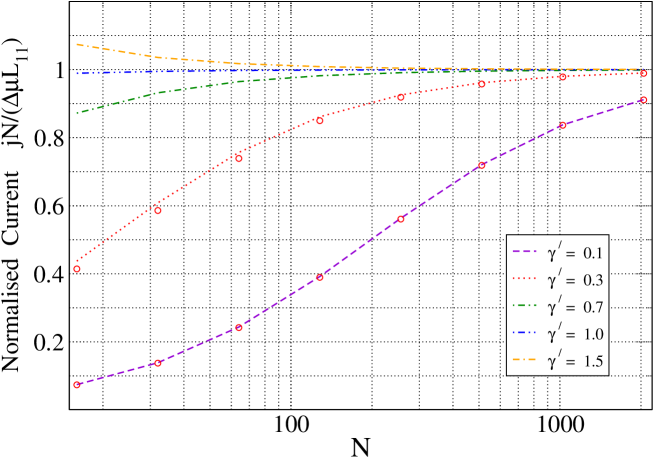
Figure 4: Plot of the normalized current versus system size for different values of the dissipation constant $\gamma^{\prime}$. The points denoted by circles correspond to the analytic scaling form given in Eq. (27).

An interesting question that is often asked in the context of mesoscopic transport is: where is the dissipation Datta (2005) ? In the case of Ohmic transport, dissipation, through Joule heat loss, takes place in the bulk of the wire. On the other hand for coherent transport there is no dissipation in the bulk of the sample and the only dissipation is at the contacts (or into the leads). This difference between Ohmic and coherent transport can be demonstrated in our model by an explicit calculation of the local heat loss at all points on the wire. Using Eq. (16) we calculate the fraction of the total heat loss that occurs at the contacts $j^{q}_{C}=j^{q}_{w-1}+j^{q}_{w-N}$ and the bulk heat loss given by $j^{q}_{B}=\sum_{l=2}^{N-1}j^{q}_{w-l}$. Note that the total dissipation is given by $\sum_{l=1}^{N}j^{q}_{w-l}=j^{p}\Delta\mu$ which easily follows from using the condition $\sum_{l=1}^{N}j^{u}_{w-l}=0$. The following table shows the contact and bulk heat losses for different system sizes and with $\gamma^{\prime}=0.1$. In this case $\ell\approx 200$. We see clearly that for $N<<\ell$ dissipation occurs mostly in the contacts to the leads while for $N>>\ell$ dissipation occurs in the bulk of the wire. Note that the heat is eventually dissipated into the reservoirs and is possible even in a steady-state scenario because of the infinite size of the reservoirs.

$L$	$j^{q}_{C}$	$j^{q}_{B}$
16	$0.9652$	$0.0348$
64	$0.8518$	$0.1482$
256	$0.5425$	$0.4575$
512	$0.3522$	$0.6478$
1024	$0.2049$	$0.7951$
2048	$0.1115$	$0.8885$

VI Discussion

An interesting aspect of the present study arises if we compare it with studies of heat transport by phonons in oscillator chains. A big question there has been to find the necessary conditions on a model of interacting particles required for the validity of Fourier’s law of heat conduction bonetto00 . As a result of a large number of studies it now appears that heat conduction in one dimensions is anomalous and Fourier’s law is not valid for momentum conserving models Lepri et al. (2003). However there are stochastic models where one can exactly demonstrate the validity of Fourier’s law. In one such model inelastic scattering of phonons take place by an exact analogue of the Büttiker probes. In this model, first proposed in [Bolsterli et al., 1970], and solved exactly recently in [Bonetto et al., 2004; Dhar and Roy, 2006] , each site on a harmonic lattice is connected to a heat reservoir whose temperature is fixed self-consistently by the condition of zero heat current. Just as Fourier’s law can be shown to hold in this model, here we have shown that both Fourier’s law and Ohm’s law are valid in the present tight-binding model. We have also been able to explicitly demonstrate local thermal equilibrium and various other linear response results. One other model where such a demonstration has been made in a clear way is the work by Larralde et al Larralde et al. (2003) on the Lorentz gas model. One other point to note is, as shown in [Dhar and Sen, 2006] , the treatments of electron and phonon transport can be done in a very similar way using the formalism of quantum Langevin equations and nonequilibrium Green’s function.

In this paper we have extended the calculation of D’Amato and Pastawski by studying the finite temperature case and considering transport of both particles and heat in a tight-binding chain. We have studied both the Ohmic and ballistic regimes. It has been shown that a simple Drude-like model of persistent random walkers can explain many of the observed features in the intermediate regime. In the Ohmic regime we have calculated verious thermoelectric coefficients and find that for certian values of the inelasticity parameter, the thermopower plotted as a function of the Fermi energy shows a peak. Finally we have explicitly computed heat dissipation in the wire.

While we have only considered the linear response regime in this paper, the formalism described here can be used to study the nonlinear regime too. Also it can be easily used to study inelastic scattering effects in the tight-binding model in any dimensions and the reservoirs themselves can be in any dimensions. Numerical implementations to study systems with Anderson type of disorder and systems with externally applied magnetic fields can also be done readily with our approach. Finally, as pointed out in the introduction, our model of inelastic scattering also serves as a model for voltage probes. An important point in experiments involving four terminal resistance measurements on quantum wires, as in [de Picciotto et al., 2001] for example, is that the voltage probe should be non-invasive. In our model the coupling to the probes can be tuned and thus can be used to obtain a better understanding of the role of probes in such experiments. Also more detailed models of the probes are easy to incorporate in our approach. The quantum Langevin method can be easily used for other models of the scattering reservoirs other than the present model where each reservoir is a one-dimensional wire. This would basically involve a change in the form of the self-energy correction. An interesting problem is an extension of the present formulation to include electron-phonon and electron-electron interactions.

VII acknowledgments

We thank Diptiman Sen and N. Kumar for useful discussions.

Appendix A Evaluation of Green’s Function

To find the Green’s function we use the relation $G^{+}_{lm}=(\hbar/\gamma)Z^{-1}_{lm}$ where $Z$ is a tridiagonal matrix with off-diagonal terms all equal to one. The diagonal terms are given by:

$$Z_{11}=Z^{+}_{NN} = A(\omega)=\frac{\hbar}{\gamma}~{}[\omega-\frac{\gamma^{2}}{\hbar^{2}}g^{+}(\omega)]$$

$$Z_{ll} = B(\omega)=\frac{\hbar}{\gamma}~{}[\omega-\frac{{\gamma^{\prime}}^{2}}{\hbar^{2}}g^{+}(\omega)]~{}~{}~{}{\rm for}~{}~{}l=2,3...N-1~{}.$$ (32)

The function $g^{+}(\omega)$ can be obtained from the green function of an isolated semi-infinite one-dimensional chain and, in the region of interest here ($|\hbar\omega|<2\gamma$) is given by

$$g^{+}(\omega)=\frac{\hbar}{\gamma}\left[\frac{\hbar\omega}{2\gamma}-i\left(1-\frac{\hbar^{2}\omega^{2}}{4\gamma^{2}}\right)^{1/2}\right]~{}.$$ (33)

Using standard matrix manipulations we can evaluate the inverse of $Z$ and find

$$Z^{-1}_{lm} = (-1)^{l+m}\frac{D_{l-1}D_{N-m}}{\Delta_{N}}~{}~{}~{}~{}{\rm for}~{}~{}m>l$$ (34)

$$= (-1)^{l+m}\frac{D_{m-1}D_{N-l}}{\Delta_{N}}~{}~{}~{}~{}{\rm for}~{}~{}m\leq l$$

$${\rm where}~{}~{}D_{l} = AY_{l-1}-Y_{l-2}$$

$$\Delta_{N} = Det[Z]={A}^{2}Y_{N-2}-2AY_{N-3}+Y_{N-4}$$

$$Y_{l} = \frac{\sinh[(l+1)\alpha]}{\sinh(\alpha)}$$

$${\rm with}~{}~{}e^{\pm\alpha} = \frac{B}{2}\pm(\frac{B^{2}}{4}-1)^{1/2}~{}.$$

We will assume that the root $\alpha$ has been chosen such that $\alpha_{R}=Re[\alpha]>0$. Using the above results for the inverse of the matrix $Z$ we find that for large $N$ the Green’s function in the wire is given by:

$$G^{+}_{lm}=\frac{(-1)^{l+m}\hbar}{2\gamma\sinh{\alpha}}~{}\left[e^{-|l-m|\alpha}-\frac{(A-e^{\alpha})}{(A-e^{-\alpha})}\left(e^{-(l+m-2)\alpha}+e^{-(2N-l-m)\alpha}\right)\right]$$ (35)

References

- Tans et al. (1997) S. J. Tans, M. H. Devoret, H. Dai, A. Thees, R. E. Smalley, L. J. Geerligs, and C. Dekker, Nature (London) 386, 474 (1997).
- Ohnishi et al. (1998) H. Ohnishi, Y. Kondo, and K. Takayanagi, Nature (London) 395, 780 (1998).
- Yanson et al. (1998) A. I. Yanson, G. Rubio Bollinger, H. E. van den Brom, N. Agraït, and J. M. van Ruitenbeek, Nature (London) 395, 783 (1998).
- de Picciotto et al. (2001) R. de Picciotto, H. L. Stormer, L. N. Pfeiffer, K. W. Baldwin, and K. W. West, Nature (London) 411, 51 (2001).
- Zimbovskaya et al. (2005) N. A. Zimbovskaya, A. T. Johnson, and N. J. Pinto, Phys. Rev. B 72, 024213 (2005).
- van Wees et al. (1988) B. J. van Wees, L. P. Kouwenhoven, D. van der Marel, H. von Houten, and C. W. J. Beenakker, Phys. Rev. Lett. 60, 848 (1988).
- Wharam et al. (1988) D. A. Wharam, T. J. Thornton, R. Newbury, M. Pepper, H. Ahmed, J. E. F. Frost, D. G. Hasko, D. C. Peacock, D. A. Ritchie, and G. A. C. Jones, J. Phys. C 21, L209 (1988).
- Gómez-Navarro et al. (2005) C. Gómez-Navarro, P. J. D. Pablo, J. Gómez-Herrero, B. Biel, F. J. Garcia-Vidal, A. Rubio, and F. Flores, Nature Materials 4, 534 (2005).
- Datta (2005) S. Datta, Quantum Transport: Atom to Transistor (Cambridge University Press, 2005).
- Agraït et al. (2002) N. Agraït, C. Untiedt, G. Rubio-Bollinger, and S. Vieira, Phys. Rev. Lett. 88, 216803 (2002).
- Park et al. (2000) H. Park, J. Park, A. K. L. Lim, E. H. Anderson, A. P. Alivisatos, and P. L. McEuen, Nature (London) 407, 57 (2000).
- (12) A. R. Champagne, A. N. Pasupathy and D.C. Ralph, Nano Lett. 5, 305 (2005).
- Ziman (1972) J. Ziman, Principles of the theory of solids (Second Edition, Cambridge University Press, 1972).
- Büttiker (1985) M. Büttiker, Phys. Rev. B 32, 1846 (1985).
- Büttiker (1986) M. Büttiker, Phys. Rev. B 33, 3020 (1986).
- D’amato and Pastawski (1990) J. L. D’amato and H. M. Pastawski, Phys. Rev. B 41, 7411 (1990).
- Maschke and Schreiber (1991) K. Maschke and M. Schreiber, Phys. Rev. B 44, 3835 (1991).
- Datta (1989) S. Datta, Phys. Rev. B 40, 5830 (1989).
- Datta and Lake (1991) S. Datta and R. K. Lake, Phys. Rev. B 44, 6538 (1991).
- Frederiksen et al. (2004) T. Frederiksen, M. Brandbyge, N. Lorente, and A.-P. Jauho, Phys. Rev. Lett. 93, 256601 (2004).
- Yamamoto et al. (2005) T. Yamamoto, K. Watanabe, and S. Watanabe, Phys. Rev. Lett. 95, 065501 (2005).
- Asai (2004) Y. Asai, Phys. Rev. Lett. 93, 246102 (2004).
- (23) K. B. Efetov, Phys. Rev. Lett. 74, 2299 (1995).
- (24) E. McCann and I. V. Lerner, J. Phys. Condens. Matter 8, 6719 (1996).
- (25) P. W. Brouwer and C. W. J. Beenakker, Phys. Rev. B 55, 4695 (1997).
- (26) C. Benjamin and A. M. Jayannavar, Phys. Rev. B 65, 153309 (2002).
- Lake and Datta (1992) R. Lake and S. Datta, Phys. Rev. B 46, 4757 (1992).
- Dhar and Sriram Shastry (2003) A. Dhar and B. Sriram Shastry, Phys. Rev. B 67, 195405 (2003).
- Dhar and Sen (2006) A. Dhar and D. Sen, Phys. Rev. B 73, 085119 (2006).
- (30) N. W. Ashcroft and N. D. Mermin, Solid state physics, (Hartcourt College Publishers, 1976).
- (31) N. F. Mott and H. Jones, The Theory of the Properties of Metals and Alloys (Clarendon, Oxford, 1936).
- (32) A. M. Lunde and K. Flensberg, J. Phys. Condens. Matter 17, 3879 (2005).
- (33) A. M. Lunde, K. Flensberg and L. I. Glazman, Phys. Rev. Lett. 97, 256802 (2006).
- (34) F. Bonetto, J. L. Lebowitz, and L. Rey-Bellet, ”Fourier’s law: a challenge for theorists”, Mathematical Physics 2000 (Imp. Coll. Press, London, 2000), math-ph/0002052.
- Lepri et al. (2003) S. Lepri, R. Livi, and A. Politi, Phys. Rep. 377, 1 (2003).
- Bolsterli et al. (1970) M. Bolsterli, M. Rich, and W. M. Visscher, Phys. Rev. A 4, 1086 (1970).
- Bonetto et al. (2004) F. Bonetto, J. L. Lebowitz, and J. Lukkarinen, J. Stat. Phys. 116, 783 (2004).
- Dhar and Roy (2006) A. Dhar and D. Roy, J. Stat. Phys. 125, 801 (2006), eprint cond-mat/0606465.
- Larralde et al. (2003) H. Larralde, F. Leyvraz, and C. Mejia-Monasterio, J. Stat. Phys. 113, 197 (2003).