Entropy in Nonequilibrium Statistical Mechanics

Abstract

Entropy in nonequilibrium statistical mechanics is investigated theoretically so as to extend the well-established equilibrium framework to open nonequilibrium systems. We first derive a microscopic expression of nonequilibrium entropy for an assembly of identical bosons/fermions interacting via a two-body potential. This is performed by starting from the Dyson equation on the Keldysh contour and following closely the procedure of Ivanov, Knoll and Voskresensky [Nucl. Phys. A 672 (2000) 313]. The obtained expression is identical in form with an exact expression of equilibrium entropy and obeys an equation of motion which satisfies the $H$-theorem in a limiting case. Thus, entropy can be defined unambiguously in nonequilibrium systems so as to embrace equilibrium statistical mechanics. This expression, however, differs from the one obtained by Ivanov et al., and we show explicitly that their “memory corrections” are not necessary. Based on our expression of nonequilibrium entropy, we then propose the following principle of maximum entropy for nonequilibrium steady states: “The state which is realized most probably among possible steady states without time evolution is the one that makes entropy maximum as a function of mechanical variables, such as the total particle number, energy, momentum, energy flux, etc.” During the course of the study, we also develop a compact real-time perturbation expansion in terms of the matrix Keldysh Green’s function.

I Introduction

Much effort has been directed towards extending equilibrium thermodynamics and statistical mechanics to open nonequilibrium systems with flows of particles, momentum and/or energy.GP71 ; Haken75 ; Kuramoto84 ; CH93 Beyond the linear-response theory,Kubo57 ; Zubarev74 however, there seems to have been yet no established theoretical framework comparable to the equilibrium one.Gibbs ; LL80 The purpose of the present paper is to make a contribution to this fundamental issue, especially on steady states without time evolution, by studying the roles of entropy in nonequilibrium statistical mechanics.

The present approach with entropy is motivated by a couple of following observations. First, equilibrium statistical mechanics is constructed on the principle of equal a priori probabilities, and the equilibrium is identified as the one which is most probable. It is hard to imagine that this concept of “maximum probability” loses its validity as soon as the system is driven from outside. For example, a gas initially prepared in one half of the container is expected to expand over the whole available space even in the presence of heat conduction through the surface. In equilibrium, it is entropy that embodies “maximum probability,” whose statistical mechanical expression is given by Boltzmann’s principle:Cercignani98

$$S_{\rm eq}\!=\!k_{\rm B}\log W\,.$$ (1)

And all the other free energies stem from $S_{\rm eq}$ through the mathematical procedure of Legendre transformations, thereby inheriting the extremum property of entropy. Thus, one may expect to have an appropriate description of open steady states by extending the concept of entropy or “maximum probability” to nonequilibrium situations. Note in this context that eq. (1), which represents the principle of equal a priori probabilities, is essentially an equilibrium expression with no dynamical equation attached to it.

The second motivation originates from the classical Boltzmann equation.CC90 ; HCB54 ; Cercignani88 ; Cercignani98 Let us define the total entropy of dilute gases by

$$S=-k_{\rm B}\int\frac{{\rm d}^{3}r{\rm d}^{3}p}{(2\pi\hbar)^{3}}\,f(\log f-1)\,,$$ (2)

where $f\!=\!f({\bm{p}},{\bm{r}},t)$ denotes the distribution function.comment1 Following the procedure to prove the $H$-theorem,Cercignani88 we then obtain the inequality:

$$\frac{{\rm d}S}{{\rm d}t}+\int{\bm{\nabla}}\cdot{\bm{j}}_{S}({\bm{r}})\,{\rm d}^{3}r\geq 0\,,$$ (3)

with ${\bm{j}}_{S}({\bm{r}})\!\equiv\!-k_{\rm B}\int\frac{{\rm d}^{3}p}{(2\pi\hbar)^{3}}\frac{{\bm{p}}}{m}f(\log f\!-\!1)$. It hence follows that ${\rm d}S/{\rm d}t\!\geq\!0$ for the isolated system. This is the usual $H$-theorem. Looking at eq. (3) more carefully, however, one may notice that ${\rm d}S/{\rm d}t\!\geq\!0$ holds whenever $\int{\bm{\nabla}}\!\cdot\!{\bm{j}}_{S}({\bm{r}}){\rm d}^{3}r\!=\!0$. Thus, entropy is expected to increase monotonically even in open systems as long as there is no net inflow or outflow of entropy through the boundary, besides those of energy, momentum and particles. This observation suggests that the open steady state, if it exists, may also correspond to the maximum of entropy with appropriately chosen independent variables. In this context, eq. (2) is superior to eq. (1) in that it is applicable to nonequilibrium systems, but inferior to eq. (1) in that it is good only for dilute classical gases.

Now, the main purposes of the present paper are twofold. First, we derive an expression of nonequilibrium entropy for an assembly of identical bosons/fermions interacting via a two-body potential so as to be compatible with equilibrium statistical mechanics. Such an investigation was performed recently for the contact interaction in a seminal paper by Ivanov, Knoll and Voskresensky.Ivanov99 ; Ivanov00 We here extend their consideration to general two-body interactions, critically reexamine their derivation,Ivanov00 and present an expression of nonequilibrium entropy which differs from theirs in an essential point. To be more specific, we adopt the nonequilibrium Dyson equation for the Keldysh matrixKeldysh64 as our starting point, which is transformed into a tractable form by the gradient expansion, i.e., the procedure well-known for a microscopic derivation of quantum transport equations.KB62 ; Keldysh64 ; Rainer83 ; RS86 ; BM90 ; LF94 ; HJ98 ; Ivanov99 ; Ivanov00 ; Kita01 An expression of nonequilibrium entropy density is then obtained from the reduced Dyson equation as eq. (71) below. It is a direct extension of eq. (2) to include both quantum and many-body effects in nonequilibrium situations, which is also compatible with the equilibrium expression.Kita99 We will show explicitly that “memory corrections” of Ivanov et al.,Ivanov00 which is the origin of the above mentioned difference in nonequilibrium entropy, are both unnecessary and incompatible with equilibrium statistical mechanics.

Second, we propose a principle of maximum entropy for nonequilibrium steady states in §IV.3. A key point is that we choose mechanical variables, such as the total particle number, energy, momentum, energy flux, etc., as independent variables of entropy. Indeed, temperature, pressure and chemical potential, which are not adopted here, are all equilibrium thermodynamic variables defined with partial derivatives of eq. (1); thus, they cannot specify any nonequilibrium state of the system. The principle may enable microscopic treatments of open steady states in exactly the same way as equilibrium systems. Its validity can only be checked by its consistency with experiments, as is the case for the principle of equal a priori probabilities in equilibrium statistical mechanics. Thus, it will be tested in the next paper on Rayleigh-Bénard convectionCH93 ; Chandrasekhar61 ; Busse78 ; Croquette89 ; Koschmieder93 ; deBruyn96 ; BPA00 of a dilute classical gas, which may be regarded as the canonical system of nonequilibrium steady states with pattern formation. It may be worth emphasizing at this stage that the present principle is connected with entropy itself. Thus, it has to be distinguished from the principle of excess entropy production by Gransdorff and Prigogine,GP71 which has been criticized by Graham,Graham81 for example; see also ref. KP98, .

During the course of study, we also develop a compact perturbation expansion on the Keldysh contour.Keldysh64 In principle, this expansion can be carried out for the round-trip Keldysh contour in the same way as in the equilibrium theory.LW60 ; AGD ; FW When writing it with respect to the real-time contour of $-\infty\!\leq\!t\!\leq\!\infty$, however, one usually has to introduce additional contour indicesKeldysh64 ; RS86 which make the actual calculations rather cumbersome and complicated. The present method will enable us to carry out the expansion on the real-time contour directly in terms of the $2\times 2$ Keldysh Green’s function without using the contour indices. Among various approximations in the perturbation expansion, we here specifically consider Baym’s $\Phi$-derivative approximation.Baym62 It has at least the following advantages: (i) it includes the exact theory; (ii) various conservation laws are automatically obeyed; (iii) the vertex corrections, or the Landau Fermi liquid corrections in a different terminology, are naturally included; (iv) $n$-particle ($n\!=\!2,3,\cdots$) correlations can also be calculated within the same approximation scheme, i.e., there is a definite prescription here to treat the Bogoliubov-Born-Green-Kirkwood-Yvons (BBGKY) hierarchy.Cercignani88 The derivation of nonequilibrium entropy by Ivanov et al. Ivanov00 will be reexamined critically within the present expansion scheme.

This paper is organized as follows. In §2, we develop a compact real-time perturbation expansion in terms of the matrix Keldysh Green’s function for an assembly of identical bosons/fermions interacting via a two-body potential. We consider the $\Phi$-derivative approximation in detail to write down the Dyson equation for the Green’s function and the expression for the two-particle correlation function. In §3, we first introduce the spectral function $A$ and the distribution function $\phi$ in the Wigner representation; they form alternative two independent components of the Keldysh Green’s function. We then carry out the first-order gradient expansion to the Dyson equation to obtain the equations for $A$ and $\phi$. In §4, we derive an expression of nonequilibrium entropy as eq. (71) below. A detailed discussion will be given on the difference between the present expression and the one obtained by Ivanov et al.Ivanov00 We then propose in §IV.3 a principle of maximum entropy for nonequilibrium steady states. Section 5 summarizes the paper. In AppendixA, we show with the present perturbation-expansion scheme that various conservation laws are automatically obeyed in the $\Phi$-derivative approximation. AppendixB presents expressions of the vertex functions in the second-order $\Phi$-derivative approximation. In AppendixC, we derive basic conservation laws in the first-order gradient expansion of the $\Phi$-derivative approximation. Finally in AppendixD, we identify the origin of the difference on equilibrium entropy between refs. Kita99, and CP75, to confirm that the “memory corrections” by Ivanov et al. Ivanov00 are unnecessary.

II Perturbation expansion with Keldysh matrix

II.1 Contour-ordered Green’s function

We consider an assembly of identical bosons/fermions whose total Hamiltonian at time $t$ is given by

$${\cal H}(t)=H_{0}+H^{\prime}(t)+H_{\rm int}a(t)\,.$$ (4)

Here $H_{0}$ denotes the kinetic energy, $H^{\prime}(t)$ is a one-body time-dependent perturbation satisfying $H^{\prime}(-\infty)\!=\!0$, $H_{\rm int}$ is a two-body interaction, and $a(t)$ is some adiabatic factor given by $a(t)\!=\!\theta(-t){\rm e}^{0_{+}t}\!+\!\theta(t)$, for example, with $\theta$ the step function and $0_{+}$ an infinitesimal positive constant. The system at $t\!=\!-\infty$ is assumed to be in some thermodynamic state described by a density matrix corresponding to $H_{0}$. Thus, we here need not consider from the beginning the contribution from the path along the imaginary time axis,RS86 ; HJ98 i.e., “initial correlation,” in the perturbation expansion with respect to $H_{\rm int}$.

The explicit expressions of $H_{0}$, $H^{\prime}(t)$ and $H_{\rm int}$ are given in second quantization by

$$H_{0}=\int\!\psi^{\dagger}({\bm{r}})\frac{-\hbar^{2}}{2m}\nabla^{2}\psi({\bm{r}})\,{\rm d}^{3}r\,,$$ (5a)

$$H^{\prime}(t)=\int\!\psi^{\dagger}({\bm{r}})U({\bm{r}},t)\psi({\bm{r}})\,{\rm d}^{3}r\,,$$ (5b)

$$H_{\rm int}=\frac{1}{2}\int\!{\rm d}^{3}r\!\int\!{\rm d}^{3}r^{\prime}V({\bm{r}}\!-\!{\bm{r}}^{\prime})\psi^{\dagger}({\bm{r}})\psi^{\dagger}({\bm{r}}^{\prime})\psi({\bm{r}}^{\prime})\psi({\bm{r}})\,.$$ (5c)

Here $m$ is the particle mass, $U$ is an external potential, and $V({\bm{r}})\!=\!V(|{\bm{r}}|)$ is a two-body interaction which can be expanded in Fourier series as

$$V({\bm{r}})=\int\!\frac{{\rm d}^{3}q}{(2\pi\hbar)^{3}}\,V_{{\bm{q}}}{\rm e}^{i{\bm{q}}\cdot{\bm{r}}/\hbar}\,.$$ (6)

The spin degrees of freedom will be suppressed for the time being.

We now adopt the interaction representation with respect to $H^{(0)}(t)\!\equiv\!H_{0}\!+\!H^{\prime}(t)$. Then, the time evolution of the system is described by the unitary operator:

$$S_{C}\equiv T_{C}\exp\left[-\frac{i}{\hbar}\int_{C}H_{\rm int}(t^{C}){\rm d}t^{C}\right].$$ (7)

Here $C$ is a round-trip contour along the real-time axis from $t\!=\!-\infty$ towards $t\!=\!\infty$,RS86 ; HJ98 $T_{C}$ denotes the contour-ordering operator along $C$, and $H_{\rm int}(t^{C})$ is the interaction representation of $H_{\rm int}a(t)$ with respect to $H^{(0)}(t)$.RS86 ; HJ98

We next introduce the contour-ordered Green’s function by

$$G(1^{C},2^{C})=-\frac{i}{\hbar}\langle T_{C}\psi_{{\cal H}}(1^{C})\psi_{{\cal H}}^{\dagger}(2^{C})\rangle\,,$$ (8)

where $\psi_{{\cal H}}(1^{C})$ is the Heisenberg operator for $\psi({\bm{r}}_{1})$ with $1^{C}\!\equiv\!{\bm{r}}_{1}t_{1}^{C}$. The perturbation expansion of $G$ with respect to $H_{\rm int}$ may be carried out in the same way as in the equilibrium theoryLW60 ; AGD ; FW by using Feynman diagrams. Indeed, one only needs to change the imaginary-time contour of the equilibrium theory into the real-time contour $C$. It hence follows that $G$ satisfies the Dyson equation:LW60

$$\left[i\hbar\frac{\partial}{\partial t_{1}^{C}}\!+\!\frac{\hbar^{2}\nabla_{1}^{2}}{2m}\!-\!U(1^{C})\right]\!G(1^{C},2^{C})$$

$$-\int\!\Sigma(1^{C},3^{C})G(3^{C},2^{C})\,{\rm d}3^{C}=\delta(1^{C},2^{C})\,,$$ (9)

where $\Sigma$ denotes the irreducible self-energy. However, the round-trip contour $C$ is not convenient for practical calculations, since time $t$ appears twice on $C$ with different orders. Thus, we usually have to introduce additional contour indices to distinguish them,Keldysh64 ; RS86 which make the actual calculations rather cumbersome and complicated.

II.2 Feynman rules in Keldysh space

It is desirable to find a simple and compact method to carry out the perturbation expansion directly on the real-time contour of $-\infty\!\leq\!t\!\leq\!\infty$. This is possible for the two-body interaction of eq. (5c) (and also for impurity potentials), as explained below. We first divide the contour $C$ into $C_{1}$ and $C_{2}$, each running from $-\infty$ to $\infty$ and from $\infty$ to $-\infty$, respectively. Accordingly, we write the integration in eq. (7) as a sum of the two contributions:

$$\int_{C}{\rm d}t^{C}=\int_{-\infty(C_{1})}^{\infty}{\rm d}t-\int_{-\infty(C_{2})}^{\infty}{\rm d}t\,.$$ (10)

We next introduce the vector:

$$\vec{\psi}(1)=\left[\begin{array}[]{c}\vspace{1mm}\psi(1^{1})\\ \psi(1^{2})\end{array}\right],\hskip 14.22636pt\vec{\psi}^{\dagger}(1)\equiv\left[\psi^{\dagger}(1^{1})\,\,\psi^{\dagger}(1^{2})\right],$$ (11)

where $\psi(1^{j})$ denotes the interaction representation of $\psi({\bm{r}}_{1})$ with $1^{j}\!\equiv\!{\bm{r}}_{1}t_{1}^{C_{j}}$. Then eq. (7) can be rewritten in terms of $\vec{\psi}^{\dagger}$, $\vec{\psi}$ and the normal-ordering operatorFW ${\cal N}$ as

$$S_{C}=T_{C}\exp\!\biggl{[}-\frac{i}{\hbar}\int{\rm d}1\int{\rm d}1^{\prime}\,\frac{{\cal N}}{2}\bar{V}(1\!-\!1^{\prime})$$

$$\hskip 28.45274pt\times\vec{\psi}^{\dagger}(1)\vec{\psi}(1)\vec{\psi}^{\dagger}(1^{\prime})\check{\tau}_{3}\vec{\psi}(1^{\prime})\biggr{]},$$ (12)

where $1\!\equiv\!{\bm{r}}_{1}t_{1}$ with $-\infty\!\leq\!t_{1}\!\leq\!\infty$, $\bar{V}$ is defined by $\bar{V}(1-1^{\prime})\!\equiv\!\delta(t_{1}-t_{1}^{\prime})V({\bm{r}}_{1}-{\bm{r}}_{1}^{\prime})$, and $\check{\tau}_{3}$ is the third Pauli matrix. The equivalence of eqs. (7) and (12) may be checked easily by writing eq. (12) without using ${\cal N}$. The interaction in eq. (12) can be expressed diagrammatically as Fig. 1. The expression (12) is quite useful for our purpose, because (i) the pairs $\vec{\psi}^{\dagger}(1)\vec{\psi}(1)$ and $\vec{\psi}^{\dagger}(1^{\prime})\check{\tau}_{3}\vec{\psi}(1^{\prime})$ can be moved around anywhere within the ${\cal N}$ and/or $T_{C}$ operators in the perturbation expansion, and (ii) a contraction of $\vec{\psi}(i)$ with $\vec{\psi}^{\dagger}(j)$ automatically yields a $2\!\times\!2$ matrix $\langle T_{C}\vec{\psi}(i)\vec{\psi}^{\dagger}(j)\rangle_{0}$, where the subscript $0$ denotes the average with respect to $H^{(0)}$. Also, the final contraction within a closed particle loop can be transformed as $\langle T_{C}\vec{\psi}^{\dagger}(i)\check{\cal M}(i,j)\vec{\psi}(j)\rangle_{0}\!=\!{\rm Tr}\check{\cal M}(i,j)\langle T_{C}\vec{\psi}(j)\vec{\psi}^{\dagger}(i)\rangle_{0}$ with $\check{\cal M}(i,j)$ denoting some matrix product of contractions.

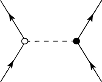
Figure 1: A diagrammatic expression of the interaction in eq. (12). The outgoing and incoming lines represent $\vec{\psi}^{\dagger}$ and $\vec{\psi}$, respectively, whereas the broken line corresponds to the interaction potential. The open and filled circles denote the unit matrix and the third Pauli matrix $\check{\tau}_{3}$, respectively.

Now, one may realize that the perturbation expansion can be carried out compactly on the real-time axis without the ambiguity on the limits of time integrationsKB62 nor the complexity from the contour indices.Keldysh64 ; RS86 We introduce the matrix Green’s function for this purpose:

$$\check{G}(1,1^{\prime})\equiv-\frac{i}{\hbar}\langle T_{C}\vec{\psi}_{\cal H}(1)\vec{\psi}_{\cal H}^{\dagger}(1^{\prime})\rangle$$

$$\hskip 4.2679pt=\left[\begin{array}[]{cc}G_{11}(1,1^{\prime})&G_{12}(1,1^{\prime})\\ G_{21}(1,1^{\prime})&G_{22}(1,1^{\prime})\end{array}\right].$$ (15)

Here $G_{12}(1,1^{\prime})\!=\!\mp(i/\hbar)\langle\psi_{\cal H}^{\dagger}(1^{\prime})\psi_{\cal H}(1)\rangle\!\equiv\!G^{<}(1,1^{\prime})$ and $G_{21}(1,1^{\prime})\!=\!-(i/\hbar)\langle\psi_{\cal H}(1)\psi_{\cal H}^{\dagger}(1^{\prime})\rangle\!\equiv\!G^{>}(1,1^{\prime})$ are the correlation functions introduced by Kadanoff and BaymKB62 with the upper (lower) sign corresponding to bosons (fermions). They satisfy

$$G_{12}(1,1^{\prime})=-G_{12}^{*}(1^{\prime},1)\,,\hskip 8.53581ptG_{21}(1,1^{\prime})=-G_{21}^{*}(1^{\prime},1)\,.$$ (16a)

The diagonal elements can be written explicitly with respect to the off-diagonal elements as

$$G_{11}(1,1^{\prime})=\theta(t_{1}^{\prime}\!-\!t_{1})G_{12}(1,1^{\prime})+\theta(t_{1}\!-\!t_{1}^{\prime})G_{21}(1,1^{\prime})\,,$$ (16b)

$$G_{22}(1,1^{\prime})=\theta(t_{1}\!-\!t_{1}^{\prime})G_{12}(1,1^{\prime})+\theta(t_{1}^{\prime}\!-\!t_{1})G_{21}(1,1^{\prime})\,,$$ (16c)

so that $G_{11}(1,1^{\prime})\!=\!-G_{22}^{*}(1^{\prime},1)$ and $G_{11}\!+\!G_{22}\!=\!G_{12}\!+\!G_{21}$. Thus, there are only two independent components in $\check{G}$, i.e., $G_{12}$ and $G_{21}$. However, all the four elements are necessary in the perturbation expansion. Equation (16) can be expressed compactly in terms of $\check{G}$ as

$$\check{G}(1,1^{\prime})=-\check{\tau}_{1}\check{G}^{\dagger}(1^{\prime},1)\check{\tau}_{1}\,,\hskip 14.22636pt{\rm Tr}\check{G}={\rm Tr}\check{G}\check{\tau}_{1}\,,$$ (17)

with $\check{\tau}_{1}$ denoting the first Pauli matrix. Equation (17) will be useful later.

The Feynman rules to calculate $\check{G}$ are summarized as follows: (i) Draw all possible $n$th-order connected diagrams. (ii) With each such diagram, associate a factor

$$\frac{(i\hbar)^{n}(\pm 1)^{\ell}}{2^{n}n!}\,,$$ (18)

where $\ell$ denotes the number of closed loops. Note that topologically identical diagrams appear $n!$ times. (iii) For each line arriving at $1$ from $2$, associate the matrix $\check{G}^{(0)}(1,2)$ or $\check{\tau}_{3}\check{G}^{(0)}(1,2)$, and multiply it from the left of the matrix arriving at $2$. (iv) If the time arguments of $\check{G}^{(0)}$ are equal, we need the replacement $G_{11}^{(0)}$, $G_{22}^{(0)}\!\rightarrow\!G_{12}^{(0)}$ due to the operator ${\cal N}$ in eq. (12). (v) Integrate and sum over all the internal variables, and take ${\rm Tr}$ for every closed particle line. (vi) The spin degrees of freedom can be included easily by multiplying every closed-loop contribution by $2S\!+\!1$, where $S$ denotes the magnitude of spin.

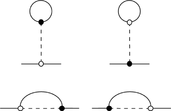
Figure 2: First-order diagrams for the matrix Green’s function.

For example, Fig. 2 enumerates topologically distinct first-order diagrams for $\check{G}$. The corresponding analytic expression is given by

$$\check{G}^{(1)}(1,1^{\prime})=\frac{i\hbar}{2}\int{\rm d}2\int{\rm d}2^{\prime}\,\bar{V}(2\!-\!2^{\prime})\bigl{\{}\pm\check{G}(1,2)$$

$$\hskip 4.2679pt\times\bigl{[}\check{G}(2,1^{\prime}){\rm Tr}\check{\tau}_{3}\check{G}(2^{\prime},2^{\prime})+\check{\tau}_{3}\check{G}(2,1^{\prime}){\rm Tr}\check{G}(2^{\prime},2^{\prime})\bigr{]}$$

$$\hskip 4.2679pt+\check{G}(1,2)\bigl{[}\check{G}(2,2^{\prime})\check{\tau}_{3}+\check{\tau}_{3}\check{G}(2,2^{\prime})\bigr{]}\check{G}(2^{\prime},1^{\prime})\bigr{\}}\,,$$ (19)

where we have replaced $\check{G}^{(0)}$ by $\check{G}$ on the right-hand side to include the renormalization effects.

The Dyson equation (9) is transformed into a matrix form as

$$\left[i\hbar\frac{\partial}{\partial t_{1}}\!+\!\frac{\hbar^{2}\nabla_{1}^{2}}{2m}\!-\!U(1)\right]\!\check{G}(1,1^{\prime})$$

$$-\int\check{\Sigma}(1,2)\check{\tau}_{3}\check{G}(2,1^{\prime})\,{\rm d}2=\delta(1,1^{\prime})\check{\tau}_{3}\,.$$ (20)

The appearance of $\check{\tau}_{3}$ between $\check{\Sigma}$ and $\check{G}$ is due to eq. (10), whereas $\check{\tau}_{3}$ in front of $\delta(1,2)$ originates from the anti-time ordering on $C_{2}$. Equation (20) is expressed alternatively in an integral form as

$$\check{G}(1,1^{\prime})=\check{G}^{(0)}(1,1^{\prime})$$

$$+\int{\rm d}2\int{\rm d}2^{\prime}\,\check{G}^{(0)}(1,2)\check{\tau}_{3}\check{\Sigma}(2,2^{\prime})\check{\tau}_{3}\check{G}(2^{\prime},1^{\prime})\,,$$ (21)

with

$$\check{G}^{(0)}(1,1^{\prime})\equiv\left[i\hbar\frac{\partial}{\partial t_{1}}+\frac{\hbar^{2}\nabla_{1}^{2}}{2m}\!-\!U(1)\right]^{-1}\delta(1,1^{\prime})\check{\tau}_{3}\,.$$ (22)

Comparing eq. (19) with the second term on the right-hand side of eq. (21), we identify the first-order self-energy with renormalization as

$$\check{\Sigma}^{(1)}(1,1^{\prime})$$

$$=\pm\frac{i\hbar}{2}\delta(1,1^{\prime})\!\int\!{\rm d}2\,\bar{V}(1\!-\!2)\bigl{[}\,\check{1}\,{\rm Tr}\check{\tau}_{3}\check{G}(2,2)+\check{\tau}_{3}{\rm Tr}\check{G}(2,2)\bigr{]}$$

$$+\frac{i\hbar}{2}\bar{V}(1\!-\!1^{\prime})\bigl{[}\check{\tau}_{3}\check{G}(1,1^{\prime})+\check{G}(1,1^{\prime})\check{\tau}_{3}\bigr{]}\,,$$ (23a)

where $$\check{1} 2\!\times\!2$$ denotes the unit matrix. One can check that the off-diagonal elements cancel out in eq. (23a). We also have to consider the Feynman rule (iv) above. Equation (23a) is thereby simplified into

$$\check{\Sigma}^{(1)}(1,1^{\prime})=\check{\tau}_{3}\Sigma^{{\rm HF}}(1,1^{\prime})\,,$$ (23b)

where $\Sigma^{{\rm HF}}$ is the Hartree-Fock self-energy:

$$\Sigma^{{\rm HF}}(1,1^{\prime})\equiv\pm\delta(1,1^{\prime})\int{\rm d}2\,\bar{V}(1\!-\!2)i\hbar G_{12}(2,2)$$

$$\hskip 28.45274pt+\bar{V}(1\!-\!1^{\prime})i\hbar G_{12}(1,1^{\prime})\,.$$ (24)

Note $\Sigma^{{\rm HF}}(1,1^{\prime})\!=\![\Sigma^{{\rm HF}}(1^{\prime},1)]^{*}$, i.e., it is Hermitian.

Thus, the above Feynman rules enable us a straightforward and automatic perturbation expansion of $\check{G}$ with neither using the contour indices nor worrying about the ordering of $T_{C}$.

II.3 $\Phi$-derivative approximation

In carrying out practical calculations, we are almost always obliged to introduce some kind of approximations. In this context, BaymBaym62 presented an extremely useful approximation scheme based on the skeleton expansion,LW60 i.e., the $\Phi$-derivative approximation. The functional $\Phi\!=\!\Phi[G]$ was introduced by Luttinger and Ward as part of the exact thermodynamic functional.LW60 The $\Phi$-derivative approximation was successively suggested by LuttingerLuttinger60 in the equilibrium theory, but has turned out to be especially useful for dynamical systems.Baym62 It has the following advantages: (i) it becomes exact if all the terms in the skeleton expansion are retained; (ii) various conservation laws, which have crucial importance to describe dynamical systems, are obeyed automatically; (iii) the vertex corrections, or the Landau Fermi liquid corrections in a different terminology, are naturally included; (iv) $n$-particle ($n\!=\!2,3,\cdots$) correlations can be obtained with the same approximation scheme, i.e., there is a definite prescription here to treat the BBGKY hierarchy.Cercignani88 A detailed study on the dynamical $\Phi$-derivative approximation has also been performed by Ivanov et al. Ivanov99 ; Ivanov00 for the contact interaction. We describe it for the general two-body interaction $V$ in terms of the present perturbation expansion scheme. It is shown explicitly in AppendixA that various conservation laws are automatically satisfied in the $\Phi$-derivative approximation.

Let us define the functional $\Phi$ in terms of eq. (12) by

$$\Phi\equiv\bigl{[}\langle\ln S_{C}\rangle_{0}-1\bigr{]}_{{\rm skeleton},\check{G}^{(0)}\rightarrow\check{G}}\,.$$ (25)

Thus, $\Phi$ formally consists of infinite closed skeleton diagrams with $\check{G}^{(0)}$ replaced by $\check{G}$.LW60 The Feynman rules to calculate $\Phi$ are exactly the same as those of $\check{G}$ which are given around eq. (18). The only care necessary is that we have $(n\!-\!1)!$ topologically identical diagrams here. The exact irreducible self-energy is obtained from $\Phi$ by

$$\check{\Sigma}(1,1^{\prime})=\pm\check{\tau}_{3}\frac{\delta\Phi}{\delta\check{G}(1^{\prime},1)}\check{\tau}_{3}\,.$$ (26)

The necessity of $\check{\tau}_{3}$ on both sides may be realized from eq. (21).

The $\Phi$-derivative approximation denotes retaining some partial diagrams from the infinite series for $\Phi$ and determining $\check{G}$ and $\check{\Sigma}$ self-consistently by eqs. (20) and (26). It follows from eqs. (17) and (26) that $\check{\Sigma}$ thus obtained also satisfies

$$\check{\Sigma}(1,1^{\prime})=-\check{\tau}_{1}\check{\Sigma}^{\dagger}(1^{\prime},1)\check{\tau}_{1}\,.$$ (27)

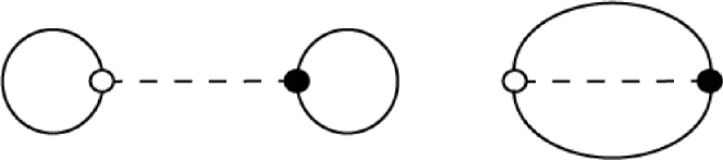
Figure 3: First-order diagrams for $\Phi$.

The first-order diagrams for $\Phi$ are given in Fig. 3. They correspond to

$$\Phi^{(1)}=\frac{i\hbar}{2}\int{\rm d}1\int{\rm d}1^{\prime}\,\bar{V}(1\!-\!1^{\prime})\left[{\rm Tr}\check{G}(1,1){\rm Tr}\check{\tau}_{3}\check{G}(1^{\prime},1^{\prime})\right.$$

$$\hskip 22.76219pt\left.\pm{\rm Tr}\check{G}(1,1^{\prime})\check{\tau}_{3}\check{G}(1^{\prime},1)\right]\,.$$ (28)

Then $\check{\Sigma}^{(1)}$ is calculated by eq. (26) to yield eq. (23a).

Next, Fig. 4 enumerates topologically distinct second-order diagrams. The corresponding analytic expression is given by

$$\Phi^{(2)}=\frac{(i\hbar)^{2}}{2^{2}2!}\int{\rm d}1\int{\rm d}1^{\prime}\int{\rm d}2\int{\rm d}2^{\prime}\,\bar{V}(1\!-\!1^{\prime})\bar{V}(2\!-\!2^{\prime})$$

$$\hskip 14.22636pt\times\bigl{[}{\rm Tr}\check{G}(1,2)\check{G}(2,1){\rm Tr}\check{\tau}_{3}\check{G}(1^{\prime},2^{\prime})\check{\tau}_{3}\check{G}(2^{\prime},1^{\prime})$$

$$\hskip 22.76219pt+{\rm Tr}\check{G}(1,2^{\prime})\check{\tau}_{3}\check{G}(2^{\prime},1){\rm Tr}\check{\tau}_{3}\check{G}(1^{\prime},2)\check{G}(2,1^{\prime})$$

$$\hskip 22.76219pt\pm 2{\rm Tr}\check{G}(1,2^{\prime})\check{\tau}_{3}\check{G}(2^{\prime},1^{\prime})\check{\tau}_{3}\check{G}(1^{\prime},2)\check{G}(2,1)\bigr{]}\,.$$ (29)

The self-energy $\check{\Sigma}^{(2)}$ is obtained by eq. (26). Expressing the result as a single matrix, we observe that the elements of $\check{\Sigma}^{(2)}$ satisfy exactly the same relations as $G_{ij}$ in eq. (16), in accordance with eq. (27). The off-diagonal elements are given by ($i\!\neq\!j$)

$$\Sigma_{ij}^{(2)}(1,1^{\prime})=\mp(\hbar)^{2}\!\int\!{\rm d}2\!\int\!{\rm d}2^{\prime}\,\bar{V}(1\!-\!2)\bar{V}(1^{\prime}\!-\!2^{\prime})$$

$$\hskip 14.22636pt\times\bigl{[}G_{ij}(1,1^{\prime})G_{ji}(2^{\prime},2)G_{ij}(2,2^{\prime})$$

$$\hskip 19.91692pt\pm G_{ij}(1,2^{\prime})G_{ji}(2^{\prime},2)G_{ij}(2,1^{\prime})\bigr{]}\,.$$ (30)

The symmetry of $\check{\Sigma}^{(2)}$ just mentioned is clearly a general property of the higher-order contributions to $\check{\Sigma}$, as may be checked order by order. Combining it with eq. (23b), we now realize that $\Sigma_{11}$ and $\Sigma_{22}$, which satisfy eq. (27), can be written more specifically as

$$\Sigma_{11}(1,1^{\prime})=\Sigma^{{\rm HF}}(1,1^{\prime})+\theta(t_{1}^{\prime}\!-\!t_{1})\Sigma_{12}(1,1^{\prime})$$

$$\hskip 22.76219pt+\theta(t_{1}\!-\!t_{1}^{\prime})\Sigma_{21}(1,1^{\prime})\,,$$ (31a)

$$\Sigma_{22}(1,1^{\prime})=-\Sigma^{{\rm HF}}(1,1^{\prime})+\theta(t_{1}\!-\!t_{1}^{\prime})\Sigma_{12}(1,1^{\prime})$$

$$\hskip 22.76219pt+\theta(t_{1}^{\prime}\!-\!t_{1})\Sigma_{21}(1,1^{\prime})\,,$$ (31b)

with $\Sigma^{{\rm HF}}$ given by eq. (24).

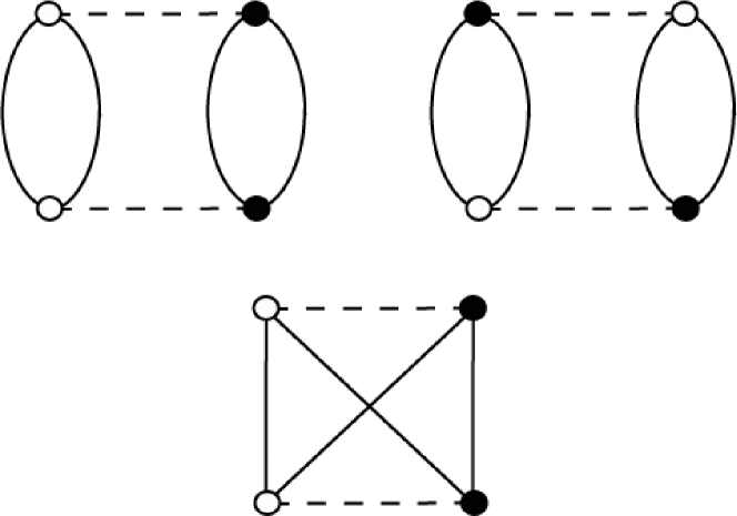
Figure 4: Topologically distinct second-order diagrams for $\Phi$.

Besides the one-particle Green’s function, the $\Phi$-derivative approximation also provides us with a definite and consistent evaluation scheme for higher-order correlations, as already shown by Baym and KadanoffKB61 and BaymBaym62 on the equilibrium imaginary-time contour. However, this topic on the Keldysh contour seems not to have been paid due attention in the literature. Especially important among them is the two-particle correlation function:

$${\cal K}_{ij,kl}(12,34)\equiv\!\left(\!-\frac{i}{\hbar}\right)^{\!\!2}\!\langle T_{C}\psi_{{\cal H}}(1^{i})\psi_{{\cal H}}(3^{k})\psi_{{\cal H}}^{\dagger}(4^{l})\psi_{{\cal H}}^{\dagger}(2^{j})\rangle$$

$$\hskip 56.9055pt-G_{ij}(1,2)G_{kl}(3,4)\,.$$ (32)

Note that the arrangement of the space-time arguments in ${\cal K}$ is different from that of Baym and Kadanoff;KB62 the present one may be more convenient when regarding ${\cal K}$ as a matrix.

To consider higher-order correlations in a unified way, we introduce an additional perturbation on the Keldysh contour caused by the non-local one-body potential $W(1^{C},2^{C})$. Adopting the interaction representation in terms of ${\cal H}$ in eq. (4), the time evolution due to $W$ is described by the operator:

$$S^{\prime}\equiv T_{C}\exp\!\left[-\frac{i}{\hbar}\int{\rm d}1\int{\rm d}1^{\prime}\,\vec{\psi}_{\cal H}^{\dagger}(1^{\prime})\check{\tau}_{3}\check{W}(1^{\prime},1)\check{\tau}_{3}\vec{\psi}_{\cal H}(1)\right],$$ (33)

where $\check{\tau}_{3}$’s originate from the transformation (10). The Green’s function is now given by

$$\check{G}(1,1^{\prime};\check{W})=-\frac{i}{\hbar}\langle T_{C}S^{\prime}\vec{\psi}_{\cal H}(1)\vec{\psi}_{\cal H}^{\dagger}(1^{\prime})\rangle/\langle T_{C}S^{\prime}\rangle\,.$$ (34)

The correlation function (32) is then obtained by

$${\cal K}_{ii^{\prime},jj^{\prime}}(11^{\prime},22^{\prime})=\!\left.\pm(-1)^{j+j^{\prime}}\frac{\delta G_{ii^{\prime}}(1,1^{\prime};\check{W})}{\delta W_{j^{\prime}j}(2^{\prime},2)}\right|_{\check{W}=\check{0}}\,,$$ (35)

where $\pm$ is due to the commutation relation between $\psi^{\dagger}$ and $\psi$, and $(-1)^{j+j^{\prime}}$ cancels the contribution of $\check{\tau}_{3}$’s in eq. (33). To calculate ${\cal K}$ self-consistently in the $\Phi$-derivative approximation, we start from the Dyson equation (20). It reads symbolically as $\check{G}^{-1}\check{G}\!=\!\check{1}$, where $\check{G}^{-1}$ is given in the present case by $\check{G}^{-1}\!=\!\check{\tau}_{3}(i\hbar\partial_{t}\!-\!K\!-\!U)\!-\!\check{\tau}_{3}(\check{W}\!+\!\check{\Sigma})\check{\tau}_{3}$ with $K$ denoting the kinetic-energy operator. Therefore, the first-order change $\delta\check{G}$ obeys $\delta\check{G}\!=\!\check{G}(-\delta\check{G}^{-1})\check{G}$. Let us substitute $-\delta\check{G}^{-1}\!=\!\check{\tau}_{3}[\delta\check{W}+(\delta\check{\Sigma}/\delta\check{G})(\delta\check{G}/\delta\check{W})\delta\check{W}]\check{\tau}_{3}$ into the first order equation and divide it by $\delta\check{W}$. We thereby obtain an integral equation for eq. (35) as

$${\cal K}_{ii^{\prime},jj^{\prime}}(11^{\prime},22^{\prime})=\pm G_{ij^{\prime}}(1,2^{\prime})G_{ji^{\prime}}(2,1^{\prime})$$

$$\pm i\hbar\sum_{kk^{\prime}ll^{\prime}}\int{\rm d}3\int{\rm d}4\int{\rm d}3^{\prime}\int{\rm d}4^{\prime}\,G_{ik^{\prime}}(1,3^{\prime})G_{ki^{\prime}}(3,1^{\prime})$$

$$\times\Gamma_{kk^{\prime},ll^{\prime}}(33^{\prime},44^{\prime}){\cal K}_{ll^{\prime},jj^{\prime}}(44^{\prime},22^{\prime})\,,$$ (36)

where $\Gamma$ is the irreducible vertex defined by

$$\Gamma_{ii^{\prime},jj^{\prime}}(11^{\prime},22^{\prime})\equiv\mp\frac{i}{\hbar}(-1)^{i+i^{\prime}}\frac{\delta\Sigma_{i^{\prime}i}(1^{\prime},1)}{\delta G_{jj^{\prime}}(2,2^{\prime})}$$

$$\hskip 34.71234pt=-\frac{i}{\hbar}\frac{\delta^{2}\Phi}{\delta G_{ii^{\prime}}(1,1^{\prime})\delta G_{jj^{\prime}}(2,2^{\prime})}\,.$$ (37)

We have used eq. (26) to derive the second expression of eq. (37). Thus, once $\Phi$ is given explicitly as a functional of $\check{G}$, the two-particle correlation (32) can also be calculated by eqs. (36) and (37).

The integral equation (36) may be solved iteratively to obtain a formal solution:

$$\check{\check{\mbox{$\cal K$}}}=\pm\bigl{(}\,\check{\check{1}}\mp i\hbar\,\check{G}\check{G}\,\check{\check{\Gamma}}\,\bigr{)}^{-1}\check{G}\check{G}\,,$$ (38)

where $\check{\check{1}}$ and $\check{G}\check{G}$ are matrices defined by

$$(\check{\check{1}})_{ii^{\prime},jj^{\prime}}(11^{\prime},22^{\prime})=\delta_{ij}\delta_{i^{\prime}j^{\prime}}\delta(1,2)\delta(1^{\prime},2^{\prime})\,,$$ (39a)

$$(\check{G}\check{G})_{ii^{\prime},jj^{\prime}}(11^{\prime},22^{\prime})=G_{ij^{\prime}}(1,2^{\prime})G_{ji^{\prime}}(2,1^{\prime})\,,$$ (39b)

respectively.

Equation (37) clearly has the symmetry:

$$\Gamma_{ii^{\prime},jj^{\prime}}(11^{\prime},22^{\prime})=\Gamma_{jj^{\prime},ii^{\prime}}(22^{\prime},11^{\prime})\,.$$ (40a)

It also follows from eq. (17) that $$\Gamma_{ii^{\prime},jj^{\prime}}$$ satisfies

$$\Gamma_{ii^{\prime},jj^{\prime}}(11^{\prime},22^{\prime})=-\sum_{kk^{\prime}ll^{\prime}}(\check{\tau}_{1})_{ik}(\check{\tau}_{1})_{k^{\prime}i^{\prime}}(\check{\tau}_{1})_{jl}(\check{\tau}_{1})_{l^{\prime}j^{\prime}}$$

$$\hskip 56.9055pt\times\,[\Gamma_{k^{\prime}k,l^{\prime}l}(1^{\prime}1,2^{\prime}2)]^{*}\,.$$ (40b)

The expressions of $\Gamma^{(n)}_{ii^{\prime},jj^{\prime}}(11^{\prime},22^{\prime})$ for $n\!=\!1,2$ are given in AppendixB to see their structures explicitly.

II.4 Keldysh transformation

As seen from eq. (16), the four elements of $\check{G}$ are not independent. This redundancy in $\check{G}$ is removed by the following modified Keldysh transformation:LO75 ; RS86

$$\check{G}^{\rm K}\equiv\check{L}\check{\tau}_{3}\check{G}\check{L}^{\dagger}=\left[\begin{array}[]{cc}G^{\rm R}&G^{\rm K}\\ 0&G^{\rm A}\end{array}\right],$$ (41)

where $\check{L}$ is defined by $\check{L}\!\equiv\!\frac{1}{\sqrt{2}}(\check{1}-i\check{\tau}_{2})$ with $\check{\tau}_{2}$ denoting the second Pauli matrix. Thus, the $21$ element of $\check{G}^{\rm K}$ vanishes, and the others also satisfy

$$[G^{{\rm R}}(1,1^{\prime})]^{*}=G^{\rm A}(1^{\prime},1)\,,\hskip 14.22636pt[G^{\rm K}(1,1^{\prime})]^{*}=-G^{\rm K}(1^{\prime},1)\,.$$ (42a)

We hence realize that $$G^{{\rm R}} G^{{\rm K}} G_{12} G_{21}$$ and form an alternative set of two independent elements in the Keldysh space. Indeed, they are connected with the Kadanoff-Baym functions and as

$$G^{{\rm R}}(1,1^{\prime})=\theta(t_{1}\!-\!t_{1}^{\prime})[G_{21}(1,1^{\prime})\!-\!G_{12}(1,1^{\prime})]\,,$$ (42b)

$$G^{{\rm K}}(1,1^{\prime})=G_{12}(1,1^{\prime})\!+\!G_{21}(1,1^{\prime})\,.$$ (42c)

It also follows from eqs. (27) and (31) that $\check{\Sigma}^{{\rm K}}\!\equiv\!\check{L}\check{\tau}_{3}\check{\Sigma}\check{L}^{\dagger}$ can be written as

$$\check{\Sigma}^{\rm K}\equiv\check{L}\check{\tau}_{3}\check{\Sigma}\check{L}^{\dagger}=\left[\begin{array}[]{cc}\Sigma^{\rm R}&\Sigma^{\rm K}\\ 0&\Sigma^{\rm A}\end{array}\right].$$ (43)

Its elements satisfy

$$[\Sigma^{{\rm R}}(1,1^{\prime})]^{*}=\Sigma^{\rm A}(1^{\prime},1)\,,\hskip 14.22636pt[\Sigma^{\rm K}(1,1^{\prime})]^{*}=-\Sigma^{\rm K}(1^{\prime},1)\,.$$ (44a)

The quantities $$\Sigma^{{\rm R}} \Sigma^{{\rm K}} \Sigma^{{\rm HF}} \Sigma_{12} \Sigma_{21}$$ and are given in terms of , and as

$$\Sigma^{{\rm R}}(1,1^{\prime})\!=\!\Sigma^{{\rm HF}}(1,1^{\prime})\!+\!\theta(t_{1}\!-\!t_{1}^{\prime})[\Sigma_{21}(1,1^{\prime})\!-\!\Sigma_{12}(1,1^{\prime})]\,,$$ (44b)

$$\Sigma^{{\rm K}}(1,1^{\prime})=\Sigma_{12}(1,1^{\prime})\!+\!\Sigma_{21}(1,1^{\prime})\,.$$ (44c)

It is worth pointing out that the Keldysh transformation is not useful in the perturbation expansions of $\check{G}$ and $\Phi$, since it obscures the basic symmetry of them. The transformation should be carried out only after finishing the expansion in terms of $\check{G}$.

Applying the Keldysh transformation to eq. (20), we obtain the Dyson equation for $\check{G}^{{\rm K}}$ as

$$\left[i\hbar\frac{\partial}{\partial t_{1}}\!+\!\frac{\hbar^{2}\nabla_{1}^{2}}{2m}\!-\!U(1)\right]\!\check{G}^{\rm K}(1,1^{\prime})$$

$$-\int\check{\Sigma}^{\rm K}(1,2)\check{G}^{\rm K}(2,1^{\prime})\,{\rm d}2=\delta(1,1^{\prime})\check{1}\,.$$ (45)

Thus, the equation for the retarded function $G^{{\rm R}}$ is completely decoupled from that of the Keldysh component $G^{{\rm K}}$.

Finally, it follows from eqs. (37), (41) and (43) that the variation $\delta\check{\Sigma}^{{\rm K}}$ is connected with $\delta\check{G}^{{\rm K}}$ as

$$\delta\Sigma_{i^{\prime}i}^{{\rm K}}(1^{\prime},1)=\pm i\hbar\sum_{jj^{\prime}}\int{\rm d}2\int{\rm d}2^{\prime}\,\Gamma_{ii^{\prime},jj^{\prime}}^{{\rm K}}(11^{\prime},22^{\prime})$$

$$\hskip 31.29802pt\times\delta G_{jj^{\prime}}^{{\rm K}}(2,2^{\prime})\,,$$ (46)

with $\Gamma_{ii^{\prime},jj^{\prime}}^{{\rm K}}$ defined by

$$\Gamma_{ii^{\prime},jj^{\prime}}^{{\rm K}}(11^{\prime},22^{\prime})\equiv\sum_{kk^{\prime}ll^{\prime}}(\check{L}\check{\tau}_{3})_{ik}(\check{L}^{\dagger})_{k^{\prime}i^{\prime}}(\check{L}\check{\tau}_{3})_{jl}(\check{L}^{\dagger})_{l^{\prime}j^{\prime}}$$

$$\hskip 56.9055pt\times\Gamma_{kk^{\prime},ll^{\prime}}(11^{\prime},22^{\prime})\,.$$ (47)

We realize from eq. (40) that $\Gamma_{ii^{\prime},jj^{\prime}}^{{\rm K}}$ satisfies

$$\Gamma_{ii^{\prime},jj^{\prime}}^{{\rm K}}(11^{\prime},22^{\prime})=\Gamma_{jj^{\prime},ii^{\prime}}^{{\rm K}}(22^{\prime},11^{\prime})\,,$$ (48a)

$$\Gamma_{ii^{\prime},jj^{\prime}}^{{\rm K}}(11^{\prime},22^{\prime})=-\sum_{kk^{\prime}ll^{\prime}}(i\check{\tau}_{2})_{ik}(i\check{\tau}_{2})_{k^{\prime}i^{\prime}}(i\check{\tau}_{2})_{jl}(\check{i\tau}_{2})_{l^{\prime}j^{\prime}}$$

$$\hskip 56.9055pt\times[\Gamma_{k^{\prime}k,l^{\prime}l}^{{\rm K}}(1^{\prime}1,2^{\prime}2)]^{*}\,.$$ (48b)

The quantity $\Gamma_{ii^{\prime},jj^{\prime}}^{{\rm K}}$ has the advantage that we only need to consider its $9$ elements instead of $16$ in $\Gamma_{ii^{\prime},jj^{\prime}}$ due to the vanishing $21$ elements in $\check{\Sigma}^{{\rm K}}$ and $\check{G}^{{\rm K}}$.

III Gradient expansion

The theoretical framework of §II enables us a formally exact microscopic treatment of nonequilibrium dynamical systems. However, the coupled equations (26) and (45) are still too difficult to solve practically. It is desirable to reduce their complexity down to a tractable level without loosing the physical essentials. To this end, we here adopt the Wigner representation and subsequently carry out the gradient expansion to eqs. (26) and (45). To be specific, the Wigner representation of $\check{G}(1,2)$ is defined through

$$\check{G}(1,2)=\int\frac{{\rm d}^{3}p\,{\rm d}\varepsilon}{(2\pi\hbar)^{4}}\check{G}({\bm{p}}\varepsilon,{\bm{r}}_{12}t_{12}){\rm e}^{i({\bm{p}}\cdot\bar{\bm{r}}_{12}-\varepsilon\bar{t}_{12})/\hbar},$$ (49)

with ${\bm{r}}_{12}\!\equiv\!({\bm{r}}_{1}\!+\!{\bm{r}}_{2})/2$, $t_{12}\!\equiv\!(t_{1}\!+\!t_{2})/2$, $\bar{\bm{r}}_{12}\!\equiv\!{\bm{r}}_{1}\!-\!{\bm{r}}_{2}$, and $\bar{t}_{12}\!\equiv\!t_{1}\!-\!t_{2}$. The gradient expansion denotes an expansion with respect to ${\bm{r}}t$ of $\check{G}({\bm{p}}\varepsilon,{\bm{r}}t)$. It forms a well-established basis for the microscopic derivation of various transport equations such as the quantumKB62 and classical Boltzmann equation. The basic assumption is that the scales of the space-time inhomogeneity are much longer than the microscopic scales to achieve the local equilibrium such as the mean-free path and the collision time. This condition is well satisfied in most of nonequilibrium steady states without time evolution such as Rayleigh-Bénard convection.CH93 ; Chandrasekhar61 ; Busse78 ; Croquette89 ; Koschmieder93 ; deBruyn96 ; BPA00

III.1 Spectral and distribution functions

As seen in eq. (16), there are essentially two independent components in $\check{G}$, i.e., $G_{12}$ and $G_{21}$. We here introduce an alternative pair of independent components, i.e., the spectral function $A$ and the distribution function $\phi$,KB62 ; Ivanov00 which turn out to be more convenient. The spectral function $A$ is defined by

$$A(1,2)\equiv i\left[G_{21}(1,2)-G_{12}(1,2)\right]$$

$$\hskip 4.2679pt=\frac{1}{\hbar}\langle\psi_{\cal H}(1)\psi_{\cal H}^{\dagger}(2)\!\mp\!\psi_{\cal H}^{\dagger}(2)\psi_{\cal H}(1)\rangle\,.$$ (50)

Let us expand $A$ as eq. (49). It then follows from the equal-time commutation relation of the field operators that $A({\bm{p}}\varepsilon,{\bm{r}}t)$ satisfies the sum rule:

$$\int_{-\infty}^{\infty}\!A({\bm{p}}\varepsilon,{\bm{r}}t)\,{\rm d}\varepsilon=2\pi\,.$$ (51)

We also conclude from $A^{*}(1,2)\!=\!A(2,1)$ that $A({\bm{p}}\varepsilon,{\bm{r}}t)$ is real. We next introduce the distribution function $\phi$ directly in the Wigner representation as

$$\phi({\bm{p}}\varepsilon,{\bm{r}}_{12}t_{12})$$

$$\equiv\frac{\displaystyle\int_{-\infty}^{\infty}\!{\rm d}\bar{t}_{12}\!\int\!{\rm d}^{3}\bar{r}_{12}\,\frac{1}{\hbar}\langle\psi^{\dagger}_{\cal H}(2)\psi_{\cal H}(1)\rangle{\rm e}^{-i({\bm{p}}\cdot\bar{\bm{r}}_{12}-\varepsilon\bar{t}_{12})/\hbar}}{A({\bm{p}}\varepsilon,{\bm{r}}_{12}t_{12})}\,.$$

(52)

We find from $A^{*}({\bm{p}}\varepsilon,{\bm{r}}t)\!=\!A({\bm{p}}\varepsilon,{\bm{r}}t)$ and $\langle\psi_{\cal H}^{\dagger}(2)\psi_{\cal H}(1)\rangle^{*}$ $=\langle\psi_{\cal H}^{\dagger}(1)\psi_{\cal H}(2)\rangle$ that $\phi({\bm{p}}\varepsilon,{\bm{r}}t)$ is also real. Thus, both $A$ and $\phi$ are real in the Wigner representation. They form an alternative pair of independent quantities in $\check{G}$.

In the equilibrium theory, $\phi$ is just the Bose/Fermi distribution function so that we only need to calculate $A$. For nonequilibrium systems, in contrast, we have to determine $A$ and $\phi$ simultaneously. The derivation of the quantum transport equationKB62 ; Keldysh64 ; Rainer83 ; RS86 ; BM90 ; LF94 ; HJ98 ; Ivanov99 ; Ivanov00 ; Kita01 amounts to integrating out the spectral function $A$, which contains detailed information on the density of states, to obtain a single equation for $\phi$. However, we shall proceed without the approximation here.

III.2 Wigner representation of $\check{G}$ and $\check{\Sigma}$

The Wigner representation of $\check{G}$ can be written in terms of $A$ and $\phi$. Indeed, the off-diagonal elements are transformed into

$$G_{12}({\bm{p}}\varepsilon,{\bm{r}}t)=\mp iA({\bm{p}}\varepsilon,{\bm{r}}t)\phi({\bm{p}}\varepsilon,{\bm{r}}t)\,,$$ (53a)

$$G_{21}({\bm{p}}\varepsilon,{\bm{r}}t)=-iA({\bm{p}}\varepsilon,{\bm{r}}t)[1\pm\phi({\bm{p}}\varepsilon,{\bm{r}}t)]\,.$$ (53b)

Using eqs. (42) and (53), we also obtain the Wigner representations of $G^{{\rm R}}$, $G^{{\rm A}}$ and $G^{{\rm K}}$ as

$$G^{{\rm R}}({\bm{p}}\varepsilon,{\bm{r}}t)=[G^{{\rm A}}({\bm{p}}\varepsilon,{\bm{r}}t)]^{*}=\int_{-\infty}^{\infty}\frac{{\rm d}\varepsilon^{\prime}}{2\pi}\,\frac{A({\bm{p}}\varepsilon^{\prime},{\bm{r}}t)}{\varepsilon_{+}-\varepsilon^{\prime}}\,,$$ (54a)

$$G^{{\rm K}}({\bm{p}}\varepsilon,{\bm{r}}t)=-iA({\bm{p}}\varepsilon,{\bm{r}}t)[1\pm 2\phi({\bm{p}}\varepsilon,{\bm{r}}t)]\,,$$ (54b)

with $\varepsilon_{+}\!\equiv\!\varepsilon\!+\!i0_{+}$. Since it may not cause any confusion, we use the same symbols $G_{ij}$ in both the coordinate and the Wigner representations. All the symbols given below without arguments belong to the Wigner representation.

Let us move on to the self-energies of eqs. (26) and (43). Following Ivanov et al.,Ivanov00 we express the Wigner representations of their independent components in a form similar to the above expressions as

$$\Sigma_{12}({\bm{p}}\varepsilon,{\bm{r}}t)=\mp iA_{\Sigma}({\bm{p}}\varepsilon,{\bm{r}}t)\phi_{\Sigma}({\bm{p}}\varepsilon,{\bm{r}}t)\,,$$ (55a)

$$\Sigma_{21}({\bm{p}}\varepsilon,{\bm{r}}t)=-iA_{\Sigma}({\bm{p}}\varepsilon,{\bm{r}}t)[1\pm\phi_{\Sigma}({\bm{p}}\varepsilon,{\bm{r}}t)]\,,$$ (55b)

and

$$\Sigma^{{\rm R}}({\bm{p}}\varepsilon,{\bm{r}}t)=[\Sigma^{{\rm A}}({\bm{p}}\varepsilon,{\bm{r}}t)]^{*}$$

$$=\Sigma^{{\rm HF}}({\bm{p}},{\bm{r}}t)+\int_{-\infty}^{\infty}\frac{{\rm d}\varepsilon^{\prime}}{2\pi}\,\frac{A_{\Sigma}({\bm{p}}\varepsilon^{\prime},{\bm{r}}t)}{\varepsilon_{+}-\varepsilon^{\prime}}\,,$$ (56a)

$$\Sigma^{{\rm K}}({\bm{p}}\varepsilon,{\bm{r}}t)=-iA_{\Sigma}({\bm{p}}\varepsilon,{\bm{r}}t)[1\pm 2\phi_{\Sigma}({\bm{p}}\varepsilon,{\bm{r}}t)]\,.$$ (56b)

It follows from eq. (27) that $A_{\Sigma}$ and $\phi_{\Sigma}$ are also real. They are functionals of $A$ and $\phi$ in the $\Phi$-derivative approximation.

The operator in the square bracket of eq. (45) can also be transformed into a matrix of the space-time coordinates by multiplying it by $\delta(1,3)$ from the right. Its Wigner representation is given by

$$G_{0}^{-1}({\bm{p}}\varepsilon,{\bm{r}}t)\equiv\varepsilon-\frac{p^{2}}{2m}-U({\bm{r}}t)\,.$$ (57)

III.3 Gradient expansion

We now consider the matrix product of the space-time coordinate. It is transformed into the Wigner representation asRS86

$$\int_{-\infty}^{\infty}\!{\rm d}\bar{t}_{12}\!\int\!{\rm d}^{3}\bar{r}_{12}\,{\rm e}^{-i({\bm{p}}\cdot\bar{\bm{r}}_{12}-\varepsilon\bar{t}_{12})/\hbar}\int{\rm d}3\,C(1,3)D(3,2)$$

$$=C({\bm{p}}\varepsilon,{\bm{r}}_{12}t_{12})\otimes D({\bm{p}}\varepsilon,{\bm{r}}_{12}t_{12})\,,$$ (58)

where the operator $\otimes$ is defined by

$$C({\bm{p}}\varepsilon,{\bm{r}}t)\!\otimes\!D({\bm{p}}\varepsilon,{\bm{r}}t)$$

$$\equiv\exp\!\left[\frac{i\hbar}{2}({\bm{\partial}}_{{\bm{r}}}\!\cdot\!{\bm{\partial}}_{{\bm{p}}^{\prime}}-\partial_{t}\partial_{\varepsilon^{\prime}}-{\bm{\partial}}_{{\bm{p}}}\!\cdot\!{\bm{\partial}}_{{\bm{r}}^{\prime}}+\partial_{\varepsilon}\partial_{t^{\prime}})\right]\!$$

$$\times C({\bm{p}}\varepsilon,{\bm{r}}t)D({\bm{p}}^{\prime}\varepsilon^{\prime},{\bm{r}}^{\prime}t^{\prime})\biggr{|}_{{\bm{p}}^{\prime}={\bm{p}},\varepsilon^{\prime}=\varepsilon,{\bm{r}}^{\prime}={\bm{r}},t^{\prime}=t}\,,$$ (59a)

with $${\bm{\partial}}_{{\bm{r}}}\!\equiv\!\partial/\partial{\bm{r}} \partial_{t}\!\equiv\!\partial/\partial t C D {\bm{r}}_{13}t_{13} {\bm{r}}_{32}t_{32} {\bm{r}}_{12}t_{12} \bar{\bm{r}}_{13}\bar{t}_{13} \bar{\bm{r}}_{32}\bar{t}_{32} \bar{\bm{r}}_{13}\,{\rm e}^{i{\bm{p}}^{\prime}\cdot\bar{\bm{r}}_{13}/\hbar}=-i\hbar\frac{\partial}{\partial{\bm{p}}^{\prime}}{\rm e}^{i{\bm{p}}^{\prime}\cdot\bar{\bm{r}}_{13}/\hbar} 3 \bar{\bm{r}}_{12}\bar{t}_{12}$$ and . The identity (58) can be proved as follows: write and on the left-hand side in the Wigner representation; expand and from ; remove and by using , etc.; perform partial integrations over internal momentum-energy variables; carry out the integrations over and . The first-order approximation to eq. (59a) yields

$$C\!\otimes\!D\approx CD+\frac{i\hbar}{2}\{C,D\}\,,$$ (59b)

where the curly bracket denotes the generalized Poisson bracket:

$$\{C,D\}\equiv\frac{\partial C}{\partial{\bm{r}}}\!\cdot\!\frac{\partial D}{\partial{\bm{p}}}-\frac{\partial C}{\partial t}\,\frac{\partial D}{\partial\varepsilon}-\frac{\partial C}{\partial{\bm{p}}}\!\cdot\!\frac{\partial D}{\partial{\bm{r}}}+\frac{\partial C}{\partial\varepsilon}\,\frac{\partial D}{\partial t}\,.$$ (60)

Finally, it should be pointed out that both the Wigner transformation (49) and the gradient expansion (58) need essential modifications in the presence of the electromagnetic field. Here we need a special care on the gauge invariance of the equations in order to appropriately obtain (i) the Hall termsHJ98 ; LF94 ; Kita01 and (ii) the pair potential of superconductivity as an effective wave function of charge $2e$.Kita01 To be specific, the Wigner transformation (49) should be defined as eq. (7) of ref. LF94, or eq. (21) of ref. Kita01, , and eq. (58) above has to be replaced by eq. (36) of ref. Kita01, .

III.4 Dyson equation in the Wigner representation

We now transform the Dyson equation into the Wigner representation within the first-order gradient expansion. Following Keldysh,Keldysh64 we start from eq. (45) rather than eq. (20) adopted by Kadanoff and BaymKB62 and Ivanov et al.Ivanov00 Indeed, eq. (45) has the advantages that (i) its $21$ element vanishes and (ii) the $22$ element is complex-conjugate of the $11$ element. Hence we essentially need to consider only the first row of eq. (45), which completely determines the two independent components of $\check{G}$, i.e., $A$ and $\phi$. Thus, we can see the structure of the equations more clearly in the present approach.

Using eq. (58) and (59b), the $11$ element of eq. (45) is transformed into

$$(G_{0}^{-1}\!-\!\Sigma^{{\rm R}})G^{{\rm R}}+\frac{i\hbar}{2}\{G_{0}^{-1}\!-\!\Sigma^{{\rm R}},G^{{\rm R}}\}=1\,,$$ (61a)

where $$G_{0}^{-1} {\rm R}\!\rightarrow\!{\rm A} 22 G^{{\rm R}}$$ is defined by eq. (57). The replacement in the superscript yields the equation for the element. Taking its complex conjugate and noting eq. (54a), we have an alternative equation for as

$$(G_{0}^{-1}\!-\!\Sigma^{{\rm R}})G^{{\rm R}}-\frac{i\hbar}{2}\{G_{0}^{-1}\!-\!\Sigma^{{\rm R}},G^{{\rm R}}\}=1\,.$$ (61b)

Let us add eqs. (61a) and (61b). We then obtain

$$G^{{\rm R}}=(G_{0}^{-1}-\Sigma^{{\rm R}})^{-1}\,.$$ (62)

We realize from eq. (54a) that this is the equation to determine the spectral function $A$ for a given $\Sigma^{{\rm R}}$. Since the $11$ and $22$ elements of eq. (45) were equivalent before the gradient expansion, it is natural to ask whether this property is still retained between eqs. (61a) and (61b). To answer the question, let us subtract eq. (61b) from eq. (61a) and substitute eq. (62) in the resulting equation. We then obtain $0=\{(G^{{\rm R}})^{-1},G^{{\rm R}}\}=-(G^{{\rm R}})^{-2}\{G^{{\rm R}},G^{{\rm R}}\}$, which is just $0\!=\!0$. We have thereby confirmed the equivalence between eqs. (61a) and (61b). We now realize that $A$ can be determined locally by eq. (62) without space-time derivatives within the first-order gradient expansion.

It follows from the retarded nature of $G^{{\rm R}}(1,2)$ in eq. (42b) that all the singularities of $G^{{\rm R}}({\bm{p}}\varepsilon,{\bm{r}}t)$ in eq. (62) lie on the lower half of the complex $\varepsilon$ plane. This implies ${\rm Im}\Sigma^{{\rm R}}({\bm{p}}\varepsilon,{\bm{r}}t)\!\leq\!0$ and hence ${\rm Im}G^{{\rm R}}({\bm{p}}\varepsilon,{\bm{r}}t)\!\leq\!0$. Using eq. (54a), the latter condition can be written alternatively as

$$A({\bm{p}}\varepsilon,{\bm{r}}t)\geq 0\,.$$ (63)

Next, the gradient expansion to the $12$ element of eq. (45) leads to

$$(G_{0}^{-1}\!-\!\Sigma^{{\rm R}})G^{{\rm K}}-\Sigma^{{\rm K}}G^{{\rm A}}+\frac{i\hbar}{2}\{G_{0}^{-1}\!-\!\Sigma^{{\rm R}},G^{{\rm K}}\}$$

$$-\frac{i\hbar}{2}\{\Sigma^{{\rm K}},G^{{\rm A}}\}=0\,.$$ (64a)

Taking its complex conjugate and using eqs. (54) and (56), we have an alternative expression of eq. (64a) as

$$(G_{0}^{-1}\!-\!\Sigma^{{\rm A}})G^{{\rm K}}-\Sigma^{{\rm K}}G^{{\rm R}}-\frac{i\hbar}{2}\{G_{0}^{-1}\!-\!\Sigma^{{\rm A}},G^{{\rm K}}\}$$

$$+\frac{i\hbar}{2}\{\Sigma^{{\rm K}},G^{{\rm R}}\}=0\,.$$ (64b)

Let us subtract eq. (64b) from eq. (64a), substitute eqs. (54) and (56) into the resulting equation, and use $\{G_{0}^{-1}\!-\!\Sigma^{{\rm R}},G^{{\rm R}}\}\!=\!0$. We thereby obtain

$$\{G_{0}^{-1}\!-\!{\rm Re}\Sigma^{{\rm R}},A\phi\}-\{A_{\Sigma}\phi_{\Sigma},{\rm Re}G^{{\rm R}}\}=\frac{AA_{\Sigma}(\phi_{\Sigma}-\phi)}{\hbar}\,.$$

The left-hand side of the equation consists of terms with space-time derivatives, whereas the right-hand side denotes the collision integral which vanishes in equilibrium. Hence it is appropriate in the first-order gradient expansion to replace $\phi_{\Sigma}$ on the left-hand side by $\phi$. The approximation was originally suggested by Botermans and MalflietBM90 and adopted explicitly by Ivanov et al.Ivanov00 The idea also has a close relationship with the Enskog series for solving the Boltzmann equation,CC90 ; HCB54 i.e., the expansion from the local equilibrium. The procedure leads to

$$\{G_{0}^{-1}\!-\!{\rm Re}\Sigma^{{\rm R}},A\phi\}-\{A_{\Sigma}\phi,{\rm Re}G^{{\rm R}}\}={\cal C}\,,$$ (65)

where ${\cal C}$ denotes the collision integral defined by

$${\cal C}\equiv\frac{AA_{\Sigma}(\phi_{\Sigma}-\phi)}{\hbar}=\mp\frac{G_{21}\Sigma_{12}-G_{12}\Sigma_{21}}{\hbar}\,.$$ (66)

Equation (65) determines $\phi$ for given $A$ and $\check{\Sigma}$.

Following Ivanov et al.,Ivanov00 we now ask the question of whether eqs. (64a) and (64b) still hold the equivalence which was present before the gradient expansion between the $12$ element of eq. (45) and its complex conjugate. Let us add eqs. (64a) and (64b). After the same procedures as above for the subtraction, we obtain

$$\frac{\{A_{\Sigma}\phi,A\}-\{A_{\Sigma},A\phi\}}{4}$$

$$=\frac{A_{\Sigma}\phi_{\Sigma}{\rm Re}G^{{\rm R}}-(G_{0}^{-1}\!-\!{\rm Re}\Sigma^{{\rm R}})A\phi}{\hbar}\,.$$

This equation is identical with eq. (65). Indeed, multiplying it by $A_{\Sigma}/(G_{0}^{-1}\!-\!{\rm Re}\Sigma^{{\rm R}})$ yields eq. (65) in disguise. This may be seen more explicitly by (i) expressing ${\rm Re}G^{{\rm R}}$ and $A$ in the two apparently different equations with respect to ${\rm Re}G^{{\rm R}-1}\!\equiv\!G_{0}^{-1}\!-\!{\rm Re}\Sigma^{{\rm R}}$ and $A_{\Sigma}$, and (ii) transforming the gradient terms into derivatives of ${\rm Re}G^{{\rm R}-1}$, $A_{\Sigma}$ and $\phi$.Ivanov00 Thus, with the approximation $\phi_{\Sigma}\!\rightarrow\!\phi$ in the gradient terms, eqs. (64a) and (64b) recover the original equivalence.

Equations (62) and (65) form coupled equations to completely determine the real quantities $A$ and $\phi$ for a given $\check{\Sigma}$. Indeed, eq. (65) is real, and the real and imaginary parts of eq. (62) are connected by the Kramers-Kronig relation.

In AppendixC, we derive basic conservation laws in the first-order gradient expansion of the $\Phi$-derivative approximation.

III.5 Self-energy in the Wigner representation

The original $\Phi$-derivative approximation denotes solving eqs. (26) and (45) self-consistently. Having performed the first-order gradient expansion to the Dyson equation (45), we also have to specify a consistent approximation scheme to the other equation (26). This issue seems not to have been given an explicit consideration before, however.

As noted below it, eq. (62) is correct up to first order in the gradient expansion. This implies that the local approximation to $\Sigma^{{\rm R}}$ is sufficient for solving eq. (62). As for eq. (65), all the terms on the left-hand side include space-time derivatives, and the collision term of the right-hand side is connected by equality with the left-hand side. Thus, eq. (65) is a first-order equation where every quantity should be evaluated locally without derivatives. With these considerations, we now conclude that we have to apply the local approximation to eq. (26). We have thereby reached the definite prescription to evaluate $\check{\Sigma}$ in terms of $\check{G}$, so that eqs. (62) and (65) now form closed equations for $A$ and $\phi$.

Using eq. (6), the Hartree-Fock self-energy (24) is transformed into the Wigner representation as

$$\Sigma^{{\rm HF}}({\bm{p}},{\bm{r}}t)=\pm i\hbar\int\!\frac{{\rm d}^{3}p^{\prime}{\rm d}\varepsilon^{\prime}}{(2\pi\hbar)^{4}}(V_{0}\pm V_{{\bm{p}}-{\bm{p}}^{\prime}})G_{12}({\bm{p}}^{\prime}\varepsilon^{\prime},{\bm{r}}t)\,.$$ (67)

Also, the local approximation to eq. (30) yields ($i\!\neq\!j$)

$$\Sigma_{ij}^{(2)}({\bm{p}}\varepsilon,{\bm{r}}t)=\mp(\hbar)^{2}\!\int\!\prod_{k=2}^{4}\frac{{\rm d}^{3}p_{k}{\rm d}\varepsilon_{k}}{(2\pi\hbar)^{4}}\frac{1}{2}|V_{{\bm{p}}-{\bm{p}}_{3}}\!\pm\!V_{{\bm{p}}-{\bm{p}}_{4}}|^{2}$$

$$\times(2\pi\hbar)^{4}\delta({\bm{p}}\!+\!{\bm{p}}_{2}\!-\!{\bm{p}}_{3}\!-\!{\bm{p}}_{4})\delta(\varepsilon\!+\!\varepsilon_{2}\!-\!\varepsilon_{3}\!-\!\varepsilon_{4})$$

$$\times G_{ji}({\bm{p}}_{2}\varepsilon_{2},{\bm{r}}t)G_{ij}({\bm{p}}_{3}\varepsilon_{3},{\bm{r}}t)G_{ij}({\bm{p}}_{4}\varepsilon_{4},{\bm{r}}t)\,.$$ (68)

Writing $G_{12}\!=\!\mp iG^{<}$, $G_{21}\!=\!-iG^{>}$, $\Sigma_{12}\!=\!\mp i\Sigma^{<}$ and $\Sigma_{21}\!=\!-i\Sigma^{>}$ in the Wigner representation, we find that eq. (68) is identical with eq. (4-16) of Kadanoff and Baym,KB62 as they should.

Contrary to the local approximation adopted here, Ivanov et al. Ivanov00 emphasized the importance of considering the first-order gradient corrections to the collision integral, which they call memory corrections. Their motivation towards this conclusion seems to be stemming from the expression of equilibrium entropy obtained by Carneiro and Pethick;CP75 see the paragraph at the end in §5.4 of Ivanov et al. Ivanov00 Indeed, they have shown that the Carneiro-Pethick expression cannot be reproduced from their dynamical equations without the memory corrections. On the other hand, we have already seen that the local approximation should be sufficient for the collision integral. Thus, one may wonder which statement is correct and where the discrepancy originates from. We will show that: (i) the Carneiro-Pethick expression of equilibrium entropy is not correct due to an inappropriate treatment of energy denominators in their calculation of the thermodynamic potential; and (ii) the local approximation without the memory corrections leads to an expression of dynamical entropy which is compatible with the equilibrium expression.Kita99 Thus, the memory corrections should not be incorporated within the first-order gradient expansion.

IV Entropy

We are now ready to discuss entropy in nonequilibrium statistical mechanics. We first derive an equation of motion for entropy density in §IV.1. We then prove the $H$-theorem for a limiting case in §IV.2. Finally, we propose a principle of maximum entropy for nonequilibrium steady states in §IV.3

IV.1 Equation of motion for entropy density

Let us multiply eq. (65) by $k_{\rm B}\ln[(1\!\pm\!\phi)/\phi]$ and integrate it over ${\bm{p}}$ and $\varepsilon$. We next write $k_{\rm B}\ln[(1\pm\phi)/\phi]{\rm d}\phi\!=\!{\rm d}\sigma$ in the resulting equation, where $\sigma$ denotes entropy of the noninteracting system:LL80

$$\sigma\equiv k_{\rm B}[-\phi\ln\phi\pm(1\pm\phi)\ln(1\pm\phi)]\,.$$ (69)

Thus, the derivatives of $\phi$ on the left-hand side are transformed into those of $\sigma$. We then perform partial integrations over ${\bm{p}}$ and $\varepsilon$. We thereby arrive at an equation of motion:

$$\frac{\partial s}{\partial t}+{\bm{\nabla}}\cdot{\bm{j}}_{s}=k_{\rm B}\hbar\!\int\!\frac{{\rm d}^{3}p\,{\rm d}\varepsilon}{(2\pi\hbar)^{4}}\,{\cal C}\ln\frac{1\pm\phi}{\phi}\,,$$ (70)

with $s\!=\!s({\bm{r}}t)$ and ${\bm{j}}_{s}\!=\!{\bm{j}}_{s}({\bm{r}}t)$ defined by

$$s\equiv\hbar\int\frac{{\rm d}^{3}p\,{\rm d}\varepsilon}{(2\pi\hbar)^{4}}\,\sigma\!\left[A\frac{\partial(G_{0}^{-1}\!-\!{\rm Re}\Sigma^{{\rm R}})}{\partial\varepsilon}+A_{\Sigma}\frac{\partial{\rm Re}G^{{\rm R}}}{\partial\varepsilon}\right],$$ (71)

$${\bm{j}}_{s}\equiv\hbar\int\frac{{\rm d}^{3}p\,{\rm d}\varepsilon}{(2\pi\hbar)^{4}}\,\sigma\!\left[-A\frac{\partial(G_{0}^{-1}\!-\!{\rm Re}\Sigma^{{\rm R}})}{\partial{\bm{p}}}-A_{\Sigma}\frac{\partial{\rm Re}G^{{\rm R}}}{\partial{\bm{p}}}\right].$$ (72)

Let us explain the quantities in these expressions once again for an easy reference. The quantity ${\cal C}$ is the collision integral (66), $\phi$ the distribution function defined by eq. (52), $A$ the Wigner transformation of eq. (50) called the spectral function, $G_{0}^{-1}$ defined by eq. (57), and the retarded functions $G^{{\rm R}}$ and $\Sigma^{{\rm R}}$ given by eqs. (54a) and (56a), respectively. The basic quantities $A$ and $\phi$ should be determined self-consistently by eqs. (62) and (65) using the self-energy of the local approximation, as discussed in detail in §III.5.

The right-hand side of eq. (70) denotes net change of entropy due to collisions, whereas $s$ and ${\bm{j}}_{s}$ on the left-hand side can be regarded as the entropy density and the entropy flux density, respectively. Indeed, eq. (71) agrees completely in form with the equilibrium expression of entropy, i.e., eq. (5) of ref. Kita99, .comment2 This may be shown explicitly from the latter by: (i) noting $\partial\phi/\partial T=-{\partial\sigma}/{\partial\varepsilon}$ for $\phi\!=\!({\rm e}^{\varepsilon/k_{\rm B}T}\!\pm\!1)^{-1}$ in equilibrium; and (ii) performing a partial integration with respect to $\varepsilon$. Thus, eq. (71) is compatible with equilibrium statistical mechanics and may be regarded as an expression of the nonequilibrium entropy density.

Equation (71) was obtained by Ivanov et al. Ivanov00 as the equation for “Markovian entropy flow.” However, they claim that there is additional contribution to entropy called “memory effects,” which originates from the gradient terms in the collision integral on the right-hand side of eq. (65). Note that the gradient terms in the collision integral have been discarded in the present formulation with rationales given in the second paragraph of §III.5. By including the memory effects, Ivanov et al. Ivanov00 could obtain an expression of entropy which is compatible with the equilibrium entropy derived earlier by Carneiro and Pethick.CP75

However, Carneiro and PethickCP75 obtained their expression with the zero-temperature time-ordered Goldstone technique where there may be ambiguity as to how to deal with vanishing energy denominators. Indeed, Carneiro and Pethick added an infinitesimal imaginary quantity to every energy denominator in their calculation of $\Phi$ in equilibrium. They thereby found a contribution to $\Phi$ from singularities in the energy denominators, i.e., the “on-energy-shell” term; see the arguments in §IV.A of their paper.CP75 It is this on-energy-shell contribution to $\Phi$ which brings the difference between eq. (71) and the Carneiro-Pethick expression.

Since the issue has a crucial importance to the whole theory, we have reexamined in AppendixD whether such singular contribution to $\Phi$ is really present or not. To this end, we adopt the finite-temperature formalism of using the Matsubara Green’s function. A definite advantage of the present approach is that no additional regularization procedure is necessary. It is thereby shown that the on-energy-shell contribution is absent. Thus, it is eq. (71) which is compatible with the equilibrium expression of entropy. The conclusion also implies that we need not consider the “memory effects” of Ivanov et al.Ivanov00

IV.2 Entropy production and the $H$-theorem

As it has already been mentioned, the right-hand side of eq. (70) expresses net change of entropy due to collisions with ${\cal C}$ given by eq. (66). We hence put

$$\mp k_{\rm B}\int\!\frac{{\rm d}^{3}p\,{\rm d}\varepsilon}{(2\pi\hbar)^{4}}\,(G_{21}\Sigma_{12}-G_{12}\Sigma_{21})\ln\frac{1\pm\phi}{\phi}\equiv\frac{\partial s_{\rm col}}{\partial t}\,,$$ (73)

and study this term more closely. It is shown shortly below that eq. (73) is positive within the second-order perturbation expansion.

Let us substitute eq. (68) into eq. (73) and rewrite it in terms of the Kadanoff-Baym functions defined in the Wigner representation byKB62 $G^{<}\!\equiv\!\pm iG_{12}\!=\!A\phi$ and $G^{>}\!\equiv\!iG_{21}\!=\!A(1\!\pm\phi)$. Equation (73) is thereby transformed into

$$\frac{\partial s_{\rm col}^{(2)}}{\partial t}=k_{\rm B}\hbar^{2}\int\prod_{j=1}^{4}\frac{{\rm d}^{3}p_{j}\,{\rm d}\varepsilon_{j}}{(2\pi\hbar)^{4}}\frac{1}{2}|V_{{\bm{p}}_{1}-{\bm{p}}_{3}}\!\pm\!V_{{\bm{p}}_{1}-{\bm{p}}_{4}}|^{2}$$

$$\hskip 2.84526pt\times(2\pi\hbar)^{4}\delta({\bm{p}}_{1}\!+\!{\bm{p}}_{2}\!-\!{\bm{p}}_{3}\!-\!{\bm{p}}_{4})\delta(\varepsilon_{1}\!+\!\varepsilon_{2}\!-\!\varepsilon_{3}\!-\!\varepsilon_{4})$$

$$\hskip 2.84526pt\times\bigl{[}G^{<}_{1}G^{>}_{2}G^{<}_{3}G^{>}_{4}-G^{>}_{1}G^{<}_{2}G^{>}_{3}G^{<}_{4}\bigr{]}\ln\frac{G^{<}_{1}G^{>}_{2}G^{<}_{3}G^{>}_{4}}{G^{>}_{1}G^{<}_{2}G^{>}_{3}G^{<}_{4}}\,,$$

(74)

with $G^{<}_{j}\!\equiv\!G^{<}({\bm{p}}_{j}\varepsilon_{j},{\bm{r}}t)$ and $G^{>}_{j}\!\equiv\!G^{>}({\bm{p}}_{j}\varepsilon_{j},{\bm{r}}t)$. Using the inequality $(x\!-\!y)\ln(x/y)\!\geq\!0$ which holds for any positive $x$ and $y$,Cercignani88 ; Cercignani98 we then conclude

$${\partial s_{\rm col}^{(2)}}({\bm{r}}t)/{\partial t}\geq 0\,.$$ (75)

Thus, entropy increases by collision in the second-order perturbation. This is quite a strong statement in that the inequality holds even locally.

The $H$-theorem is relevant to the space integral of eq. (70) over the whole system:Cercignani88 ; Cercignani98

$$\frac{{\rm d}}{{\rm d}t}\int s({\bm{r}}t)\,{\rm d}^{3}r+\int{\bm{j}}_{s}({\bm{r}}t)\cdot{\rm d}{\bm{S}}=\frac{{\rm d}}{{\rm d}t}\int s_{\rm col}({\bm{r}}t)\,{\rm d}^{3}r\,,$$ (76)

where ${\rm d}{\bm{S}}$ denotes the infinitesimal surface element. We review it here for a later extension: Consider an isolated system where the second term on the left-hand side vanishes. If the time evolution of entropy by collision is globally positive, i.e.,

$$\frac{{\rm d}}{{\rm d}t}\int s_{\rm col}({\bm{r}}t)\,{\rm d}^{3}r\geq 0\,,$$ (77)

we obtain the law of increase of entropy for the relevant system as

$$\frac{{\rm d}}{{\rm d}t}\int s({\bm{r}}t)\,{\rm d}^{3}r\geq 0\,.$$ (78)

It hence follows that entropy takes its maximum value in equilibrium of an isolated system.

There seems to have been yet no explicit proof for eq. (77) beyond the second-order perturbation. Indeed, the $H$-theorem has been discussed almost exclusively in terms of the Boltzmann equation with the two-particle (i.e., second-order) collision integral. A general expression corresponding to eq. (74) has been provided for the contact interaction as eq. (5.11) of Ivanov et al.Ivanov00 A sufficient condition for the general $H$-theorem to hold is $R_{m,m^{\prime}}\!\geq\!0$ in their expression at every order of the perturbation expansion, which seems nontrivial to prove at present and we defer it for a future study. However, it should be noted that Nature clearly adopts the inequality (77) beyond the second-order, since no explicit violation of the second law of thermodynamics has been reported even in systems with strong correlations. See also the numerical work by Orban and Bellemans on the time evolution of entropy of an isolated system.OB67

IV.3 Maximum entropy in nonequilibrium steady states

We now extend the above principle of maximum entropy to nonequilibrium steady states without time evolution. We consider specifically those cases where there is influx of current $J_{z}$ and/or energy current $J_{\varepsilon z}$ through one boundary perpendicular to the $z$ axis. It follows from the conservation laws that there is the same amount of currents flowing out through another boundary in the steady state; hence these quantities can surely be adopted as additional variables of entropy to specify the system.

First of all, we assume that eq. (77) also holds in steady states. This can be proved explicitly within the second-order perturbation as eq. (75). Next, we note that there is no net inflow or outflow of entropy in steady states as well, i.e., the second term on the left-hand side of eq. (76) vanishes. Hence it is quite reasonable to expect that eq. (78) also holds for steady states under appropriate conditions. The question then arises: what are the parameters that have to be fixed? In this context, we note that the principle of maximum entropy in equilibrium can be stated without the magic word of “isolated system” as $S_{\rm eq}(E,V,N)\!=\!{\rm maximum}$, where energy $E$, volume $V$ and number $N$ are all mechanical variables. This is quite natural, since “probability” can only be introduced at first in terms of mechanical variables. In contrast, temperature $T$, pressure $p$ and chemical potential $\mu$ are all equilibrium thermodynamic variables defined in terms of $S_{\rm eq}$ by partial differentiations, i.e., there are no definite definitions for them in nonequilibrium. Hence the latter cannot specify nonequilibrium states of the system. These considerations indicate that we should choose mechanical variables as independent variables of nonequilibrium entropy. We hence add $J_{z}$ and $J_{\varepsilon z}$, which are conserved and can be calculated mechanically, as independent variables of entropy in the present context. Now, we extend the principle of maximum entropy as follows:

Principle of maximum entropy for steady states: The state which is realized most probably among possible steady states without time evolution is the one that makes $S(E,V,N,J_{z},J_{\varepsilon z})$ maximum.

The validity of the principle can only be checked by its consistency with experiments. In the next paper we shall test it on Rayleigh-Bénard convection of a dilute classical gas which is typical of nonequilibrium steady states with pattern formation.CH93 ; Chandrasekhar61 ; Busse78 ; Croquette89 ; Koschmieder93 ; deBruyn96 ; BPA00 It will be shown that the convection indeed gives rise to an increase of entropy over the value of the heat conducting state.

Finally, it may be worth pointing out that, once $S(E,V,N,J_{z},J_{\varepsilon z})$ is given explicitly, we may perform successive Legendre transformations to change independent variables, just as in the equilibrium theory.

V Summary

We have performed a theoretical study on entropy in nonequilibrium statistical mechanics by specifically considering an assembly of identical bosons/fermions interacting via a two-body potential. First, we have presented an expression of nonequilibrium entropy density as eq. (71), which obeys the equation of motion (70). Thus, we can now trace time evolution of entropy in the many-body system. Second, we have proposed a principle of maximum entropy in §IV.3 for nonequilibrium steady states without time evolution. The validity of the principle will be checked in the next paper by calculating the entropy change of a dilute classical gas through the Rayleigh-Bénard convective transition.

A conventional theoretical starting point to nonequilibrium systems has been some phenomenological deterministic equations connected closely with the conservation laws.CH93 One then performs the linear stability analysis and derives some effective equations near the instability point such as “amplitude equations” or “phase equations.” In some fortunate cases one may further be able to construct a Lyapunov function from those differential equations.CH93 Note however that this approach is essentially of mechanical character, as it is completely irrelevant to the concept of probability. In contrast, little attention seems to have been paid to entropy in nonequilibrium systems, even near instability points, due partly to the absence of an explicit expression of nonequilibrium entropy. Since entropy is the key concept of equilibrium thermodynamics and statistical mechanics embodying “probability,” it will be well worth studying entropy of nonequilibrium systems and their “phase transitions,” which will shed new light on the phenomena. The theoretical framework proposed here may provide a starting point for those investigations. Its obvious advantage over the approach of the nonequilibrium statistical operator by ZubarevZubarev74 is that one can treat nonequilibrium systems which are globally far away from equilibrium, though not locally.

Homogeneity/additivity has played a key role in constructing equilibrium statistical mechanics. In contrast, the present approach may be regarded as an attempt to treat open inhomogeneous systems by an extremum principle with considering the boundary conditions explicitly. Once it is established that steady states are identified correctly with the extremum principle, it will be a straightforward task to develop the linear-response theory around it in the same way as in the equilibrium theory.Kubo57 ; Zubarev74

Appendix A Conservation Laws

We here show in terms of the present real-time perturbation expansion in the Keldysh space that various conservation laws are automatically satisfied in the $\Phi$-derivative approximation. We follow essentially the procedures by BaymBaym62 with a slight modification appropriate for the real-time contour.

A.1 Identities

To start with, we derive several identities which form the basis for proving the conservation laws.

First, consider the following gauge transformation:

$$\check{G}(2,1)\longrightarrow{\rm e}^{i\check{\chi}(2)}\check{G}(2,1){\rm e}^{-i\check{\chi}(1)}\,,$$ (79a)

with

$$\check{\chi}(1)\equiv\left[\begin{array}[]{cc}\chi(1)&0\\ 0&0\end{array}\right].$$ (79b)

It yields a first-order change in $\check{G}$ as

$$\delta\check{G}(2,1)=i\left[\check{\chi}(2)\check{G}(2,1)-\check{G}(2,1)\check{\chi}(1)\right]\,.$$ (80)

However, $\Phi$ is clearly invariant through eq. (79). With eq. (26), this invariance of $\Phi$ reads

$$\int\!{\rm d}1\!\int\!{\rm d}2\,{\rm Tr}\check{\tau}_{3}\check{\Sigma}(1,2)\check{\tau}_{3}\delta\check{G}(2,1)=0\,.$$ (81)

Substituting eq. (80) into eq. (81) and using $\chi(1)$ is arbitrary, we obtain

$$\int\!{\rm d}2\,{\rm Tr}\,\frac{\check{1}\!+\!\check{\tau}_{3}}{2}\bigl{[}\check{\tau}_{3}\check{\Sigma}(1,2)\check{\tau}_{3}\check{G}(2,1)-\check{G}(1,2)\check{\tau}_{3}\check{\Sigma}(2,1)\check{\tau}_{3}\bigr{]}$$

$$=0\,.$$ (82a)

We can further transform eq. (82a) into

$$\int\!{\rm d}2\,\bigl{[}\Sigma^{{\rm R}}(1,2)G_{12}(2,1)+\Sigma_{12}(1,2)G^{{\rm A}}(2,1)$$

$$-G^{{\rm R}}(1,2)\Sigma_{12}(2,1)-G_{12}(1,2)\Sigma^{{\rm A}}(2,1)\bigr{]}=0\,,$$ (82b)

where we have used eqs. (16b), (31a), (42b), (44b) and the Feynman rule (iv) around eq. (18). This is the basic identity obtained with respect to the gauge transformation.

Second, consider the following Galilean transformation:

$$\check{G}(2,1)\longrightarrow\exp\!\left[\check{\bm{R}}(t_{2})\!\cdot\!\overrightarrow{\mbox{\boldmath$\nabla$}}_{2}\right]\check{G}(2,1)\exp\!\left[\overleftarrow{\mbox{\boldmath$\nabla$}}_{1}\!\cdot\!\check{\bm{R}}(t_{1})\right]\,,$$ (83a)

with

$$\check{\bm{R}}(t)\equiv\left[\begin{array}[]{cc}{\bm{R}}(t)&{\bm{0}}\\ {\bm{0}}&{\bm{0}}\end{array}\right].$$ (83b)

It yields the following first-order change:

$$\delta\check{G}(2,1)=\check{\bm{R}}(t_{2})\!\cdot\!{\mbox{\boldmath$\nabla$}}_{2}\check{G}(2,1)+\check{\bm{R}}(t_{1})\!\cdot\!{\mbox{\boldmath$\nabla$}}_{1}\check{G}(2,1)\,.$$ (84)

However, $\Phi$ is invariant through eq. (83) so that eq. (81) holds also in this case. Substituting (84) into eq. (81) and using ${\bm{R}}(t)$ is arbitrary, we obtain

$$\!\int\!{\bm{Q}}(1)\,{\rm d}^{3}r_{1}={\bm{0}}\,,$$ (85)

with ${\bm{Q}}(1)$ defined by

$${\bm{Q}}(1)\equiv\mp i\hbar\frac{\mbox{\boldmath$\nabla$}_{\!1}\!-\!\mbox{\boldmath$\nabla$}_{\!1^{\prime}}}{2}\!\int\!{\rm d}2\,\bigl{[}\Sigma^{\rm R}(1,2)G_{12}(2,1^{\prime})$$

$$\hskip 2.84526pt+\Sigma_{12}(1,2)G^{\rm A}(2,1^{\prime})-G^{\rm R}(1,2)\Sigma_{12}(2,1^{\prime})$$

$$\hskip 2.84526pt-G_{12}(1,2)\Sigma^{\rm A}(2,1^{\prime})\bigr{]}_{1^{\prime}=1}\,.$$ (86)

Here terms with the self-energy derivative are due to partial integrations. Equation (85) is the identity obtained in terms of the Galilean transformation.

We finally consider the change of time on $C_{1}$: $t\!\rightarrow\!\theta(t)\!\equiv\!t\!+\!\varphi(t)$. Accordingly, $\check{G}$ is transformed as

$$\check{G}(2,1)\longrightarrow\!\check{U}(t_{2})\check{G}({\bm{r}}_{2}\theta_{2},{\bm{r}}_{1}\theta_{1})\check{U}(t_{1})\,,$$ (87a)

with

$$\check{U}(t)\equiv\left[\begin{array}[]{cc}({\rm d}\theta/{\rm d}t)^{1/4}&0\\ 0&0\end{array}\right].$$ (87b)

The factor $({\rm d}\theta/{\rm d}t)^{1/4}$ cancels the Jacobian for $t\!\rightarrow\!\theta$ in eq. (12), thereby keeping $\Phi$ invariant in form. We hence conclude that eq. (81) also holds in this case. The first-order change in $\check{G}$ is given explicitly by

$$\delta G_{ji}(2,1)=\left\{\delta_{j1}\!\left[\frac{\varphi^{\prime}(t_{2})}{4}\!+\!\varphi(t_{2})\frac{\partial}{\partial t_{2}}\right]\right.$$

$$\hskip 11.38109pt\left.+\delta_{i1}\!\left[\frac{\varphi^{\prime}(t_{1})}{4}+\varphi(t_{1})\frac{\partial}{\partial t_{1}}\right]\!\right\}G_{ji}(2,1)\,.$$ (88)

Substituting eq. (88) into eq. (81) and using $\varphi(t)$ is arbitrary, we obtain

$$\frac{{\rm d}\langle H_{\rm int}(t_{1})\rangle}{{\rm d}t_{1}}=-\int\!Q_{\varepsilon}(1)\,{\rm d}^{3}r_{1}\,,$$ (89)

where $\langle H_{\rm int}(t_{1})\rangle$ and $Q_{\varepsilon}(1)$ are defined by

$$\langle H_{\rm int}(t_{1})\rangle=\pm\frac{i\hbar}{4}\int\!{\rm d}^{3}r_{1}\!\int\!{\rm d}2\,\bigl{[}\Sigma^{\rm R}(1,2)G_{12}(2,1)$$

$$\hskip 27.0301pt+\Sigma_{12}(1,2)G^{\rm A}(2,1)+G^{\rm R}(1,2)\Sigma_{12}(2,1)$$

$$\hskip 27.0301pt+G_{12}(1,2)\Sigma^{\rm A}(2,1)\bigr{]}\,,$$ (90)

$$Q_{\varepsilon}(1)\equiv(\mp i\hbar)\frac{\partial}{\partial t_{1}}\!\int\!{\rm d}2\,\bigl{[}\Sigma^{\rm R}(1^{\prime},2)G_{12}(2,1)$$

$$\hskip 11.38109pt+\Sigma_{12}(1^{\prime},2)G^{\rm A}(2,1)+G^{\rm R}(1,2)\Sigma_{12}(2,1^{\prime})$$

$$\hskip 11.38109pt+G_{12}(1,2)\Sigma^{\rm A}(2,1^{\prime})\bigr{]}_{1^{\prime}=1}\,,$$ (91)

respectively. Equation (89) is the identity obtained from eq. (87).

It should be noted that $\langle H_{\rm int}(t_{1})\rangle$ defined above is exactly the interaction energy of the system. This can be seen as follows: With eqs. (16), (31), (42b) and (44b), the $12$ element of eq. (20) is transformed into

$$\left[i\hbar\frac{\partial}{\partial t_{1}}\!+\!\frac{\hbar^{2}\nabla_{1}^{2}}{2m}\!-\!U(1)\right]\!G_{12}(1,2)-\int\!\left[\Sigma^{{\rm R}}(1,3)G_{12}(3,2)\right.$$

$$\left.+\,\Sigma_{12}(1,3)G^{{\rm A}}(3,2)\right]{\rm d}3=0\,.$$ (92)

We may alternatively derive an equation for $G_{12}(1,2)\!=\!\mp(i/\hbar)\langle\psi_{\cal H}^{\dagger}(2)\psi_{\cal H}(1)\rangle$ starting from the equation of motion for $\psi_{\cal H}(1)$:

$$\!\left[i\hbar\frac{\partial}{\partial t_{1}}+\frac{\hbar^{2}\nabla_{1}^{2}}{2m}-U(1)\right]\!\psi_{\cal H}(1)$$

$$-\int{\rm d}1^{\prime}\,\bar{V}(1\!-\!1^{\prime})\psi_{\cal H}^{\dagger}(1^{\prime})\psi_{\cal H}(1^{\prime})\psi_{\cal H}(1)=0\,.$$ (93)

Let us multiply eq. (93) by $(\mp i/\hbar)\psi_{\cal H}^{\dagger}(2)$ from the left, take its thermodynamic average, and compare the result with eq. (92). We then obtain the identity:

$$\int{\rm d}1^{\prime}\,\bar{V}(1\!-\!1^{\prime})\langle\psi_{\cal H}^{\dagger}(2)\psi_{\cal H}^{\dagger}(1^{\prime})\psi_{\cal H}(1^{\prime})\psi_{\cal H}(1)\rangle$$

$$=\pm i\hbar\int\!\!\left[\Sigma^{{\rm R}}(1,3)G_{12}(3,2)\!+\!\Sigma_{12}(1,3)G^{{\rm A}}(3,2)\right]{\rm d}3\,.$$

(94)

Setting $2\!=\!1$ in eq. (94) yields an expression of the interaction energy in terms of the self-energy. An alternative expression is obtained by taking its complex conjugate. We thereby conclude that eq. (90) is indeed the interaction energy of the system.

A.2 Conservation laws

We are now ready to prove that the conservation laws are automatically satisfied in the $\Phi$-derivative approximation.

Let us take complex conjugate of eq. (92) and use eqs. (16a), (27), (42a) and (44a). This yields

$$\left[-i\hbar\frac{\partial}{\partial t_{2}}\!+\!\frac{\hbar^{2}\nabla_{2}^{2}}{2m}\!-\!U(2)\right]\!G_{12}(1,2)-\!\int\!\!\left[G^{{\rm R}}(1,3)\Sigma_{12}(3,2)\!\right.$$

$$\left.+\,G_{12}(1,3)\Sigma^{{\rm A}}(3,2)\right]{\rm d}3=0\,.$$ (95)

First, we subtract eq. (95) from eq. (92), set $2\!=\!1$, and use the identity (82b). We thereby obtain the number conservation law as

$$\frac{\partial n(1)}{\partial t_{1}}+{\bm{\nabla}}_{1}\!\cdot{\bm{j}}(1)=0\,,$$ (96)

where $n(1)$ and ${\bm{j}}(1)$ are the particle and current densities defined by

$$n(1)\equiv\pm i\hbar G_{12}(1,1)\,,$$ (97a)

$${\bm{j}}(1)\equiv\left.\pm\hbar^{2}\frac{{\bm{\nabla}}_{1}\!-\!{\bm{\nabla}}_{2}}{2m}G_{12}(1,2)\right|_{2=1}\,,$$ (97b)

respectively.

We next operate $\mp i\hbar({\bm{\nabla}}_{1}\!-\!{\bm{\nabla}}_{2})/2m$ to eqs. (92) and (95), subtract the latter from the former, and set $2\!=\!1$. We thereby find that the time evolution of the current density obeys

$$\frac{\partial}{\partial t_{1}}{\bm{j}}(1)+\frac{1}{m}{\bm{\nabla}}_{1}\underline{\Theta}^{K}(1)+\frac{n(1)}{m}{\bm{\nabla}}_{1}U(1)=\frac{1}{m}{\bm{Q}}(1)\,,$$ (98)

where ${\bm{Q}}(1)$ is given by eq. (86), and tensor $\underline{\Theta}^{K}(1)$ is defined by

$$\Theta_{ij}^{K}(1)=\mp\frac{i\hbar^{3}}{4m}(\nabla_{\!1i}\!-\!\nabla_{\!2i})(\nabla_{\!1j}\!-\!\nabla_{\!2j})G_{12}(1,2)\bigr{|}_{2=1}\,.$$ (99)

Integrating eq. (98) over the whole space of the relevant system and using eq. (85), we obtain the total momentum conservation law as

$$\frac{\partial}{\partial t_{1}}\!\int\!{\bm{j}}(1)\,{\rm d}^{3}r_{1}=-\!\int\!\frac{n(1)}{m}{\bm{\nabla}}_{1}U(1)\,{\rm d}^{3}r_{1}\,.$$ (100)

We finally operate $\mp i\hbar\frac{\partial}{\partial t_{2}}$ and $\mp i\hbar\frac{\partial}{\partial t_{1}}$ to eqs. (92) and (95), respectively. Adding the resulting equations and setting $2\!=\!1$, we obtain

$$\frac{\partial{\cal E}_{{\rm K}}(1)}{\partial t_{1}}+{\bm{\nabla}}_{1}\cdot{\bm{j}}_{\varepsilon}^{\prime}(1)+U(1)\frac{\partial n(1)}{\partial t_{1}}=Q_{\varepsilon}(1)\,,$$ (101)

where $Q_{\varepsilon}(1)$ is given by eq. (91), and ${\cal E}_{{\rm K}}(1)$ and ${\bm{j}}_{\varepsilon}^{\prime}(1)$ are defined by

$${\cal E}_{{\rm K}}(1)\equiv\pm\frac{i\hbar^{3}}{2m}{\bm{\nabla}}_{1}\!\cdot\!{\bm{\nabla}}_{2}G_{12}(1,2)\biggr{|}_{2=1}\,,$$ (102)

$${\bm{j}}_{\varepsilon}^{\prime}(1)=\mp\frac{i\hbar^{3}}{2m}\!\left(\frac{\partial}{\partial t_{1}}{\bm{\nabla}}_{2}\!+\!\frac{\partial}{\partial t_{2}}{\bm{\nabla}}_{1}\right)\!G_{12}(1,2)\biggr{|}_{2=1}\,,$$ (103)

respectively. The quantity ${\cal E}_{{\rm K}}(1)$ denotes the kinetic energy density. We next integrate eq. (101) over space and use eqs. (89) and (96). We thereby obtain the total-energy conservation law as

$$\frac{{\rm d}}{{\rm d}t_{1}}\!\left[\int\!{\cal E}_{{\rm K}}(1)\,{\rm d}^{3}r_{1}\!+\!\langle H_{\rm int}(t_{1})\rangle\right]\!=-\!\int\!{\bm{j}}(1)\cdot\!{\bm{\nabla}}_{1}U(1)\,{\rm d}^{3}r_{1}\,.$$ (104)

Thus, the conservation laws are automatically satisfied in the $\Phi$-derivative approximation as eqs. (96), (100) and (104).

Appendix B Expression of $\Gamma$

We here present expressions of the vertex function (37) within the second-order skeleton expansion by using eqs. (28) and (29). This will help us to understand the structures of $\Gamma$.

First, $\Gamma^{(1)}_{ii^{\prime},jj^{\prime}}$ is obtained from eq. (28) with eq. (37). It may be written compactly as

$$\Gamma^{(1)}_{ii^{\prime},jj^{\prime}}(11^{\prime},22^{\prime})=\bar{V}(1\!-\!2)\delta_{ij}\delta_{i^{\prime}j^{\prime}}(\check{\tau}_{3})_{ii^{\prime}}[\delta(1,1^{\prime})\delta(2,2^{\prime})$$

$$\hskip 65.44133pt\pm\delta(1,2^{\prime})\delta(2,1^{\prime})]\,.$$ (105)

Thus, only $\Gamma^{(1)}_{11,11}=-\Gamma^{(1)}_{22,22}$ are finite among $\Gamma^{(1)}_{ii^{\prime},jj^{\prime}}$.

Second, $\Gamma^{(2)}_{ii^{\prime},jj^{\prime}}$ is calculated from eq. (29). It turns out that only $\Gamma^{(2)}_{ij,ij}$ and $\Gamma^{(2)}_{ij,ji}$ are finite. For $i\!\neq\!j$, they are given by

$$\Gamma^{(2)}_{ij,ij}(11^{\prime},22^{\prime})=-i\hbar\bar{V}(1\!-\!2)\bar{V}(1^{\prime}\!-\!2^{\prime})[G_{ji}(1^{\prime},1)$$

$$\times G_{ji}(2^{\prime},2)\pm G_{ji}(1^{\prime},2)G_{ji}(2^{\prime},1)]\,,$$ (106a)

$$\Gamma^{(2)}_{ij,ji}(11^{\prime},22^{\prime})$$

$$=-i\hbar\biggl{[}\bar{V}(1^{\prime}\!-\!2)\bar{V}(1\!-\!2^{\prime})G_{ji}(1^{\prime},1)G_{ij}(2^{\prime},2)$$

$$+\delta(1^{\prime},2)\delta(1,2^{\prime})\!\int\!{\rm d}3\!\int\!{\rm d}3^{\prime}\,\bar{V}(1^{\prime}\!-\!3)\bar{V}(1\!-\!3^{\prime})$$

$$\hskip 56.9055pt\times G_{ji}(3,3^{\prime})G_{ij}(3^{\prime},3)$$

$$\pm\delta(1^{\prime},2)\bar{V}(1\!-\!2^{\prime})\!\int\!{\rm d}3\,\bar{V}(1^{\prime}\!-\!3)G_{ij}(2^{\prime},3)G_{ji}(3,1)$$

$$\pm\bar{V}(1^{\prime}\!-\!2)\delta(1,2^{\prime})\!\int\!{\rm d}3\,\bar{V}(1\!-\!3)G_{ji}(1^{\prime},3)G_{ij}(3,2)\biggr{]}\,,$$

(106b)

respectively. Also, $$\Gamma^{(2)}_{ii,ii}$$ is given in terms of the above quantities as

$$\Gamma^{(2)}_{11,11}(11^{\prime},22^{\prime})=-\Gamma^{(2)*}_{22,22}(1^{\prime}1,2^{\prime}2)$$

$$=-\theta(t_{1}^{\prime}-t_{1})\theta(t_{2}^{\prime}-t_{2})\Gamma^{(2)}_{12,12}(11^{\prime},22^{\prime})$$

$$-\theta(t_{1}^{\prime}-t_{1})\theta(t_{2}-t_{2}^{\prime})\Gamma^{(2)}_{12,21}(11^{\prime},22^{\prime})$$

$$-\theta(t_{1}-t_{1}^{\prime})\theta(t_{2}-t_{2}^{\prime})\Gamma^{(2)}_{21,21}(11^{\prime},22^{\prime})$$

$$-\theta(t_{1}-t_{1}^{\prime})\theta(t_{2}^{\prime}-t_{2})\Gamma^{(2)}_{21,12}(11^{\prime},22^{\prime})\,.$$ (106c)

These are the expressions of $\Gamma^{(n)}_{ii^{\prime},jj^{\prime}}$ for $n\!=\!1,2$ in the space-time coordinates.

We next write down $\Gamma_{ii^{\prime},jj^{\prime}}(11^{\prime},22^{\prime})$ of the local approximation which will be necessary later. In this case, $\Gamma_{ii^{\prime},jj^{\prime}}(11^{\prime},22^{\prime})$ acquires the structure of the uniform system. To be specific, we substitute eq. (49) into eq. (37) and adopt the local approximation. We then find order by order that $\Gamma_{ii^{\prime},jj^{\prime}}(11^{\prime},22^{\prime})$ can be expanded as

$$\Gamma_{ii^{\prime},jj^{\prime}}(11^{\prime},22^{\prime})$$

$$=\int\frac{{\rm d}^{3}p_{1}{\rm d}\varepsilon_{1}}{(2\pi\hbar)^{4}}\int\frac{{\rm d}^{3}p_{2}{\rm d}\varepsilon_{2}}{(2\pi\hbar)^{4}}\int\frac{{\rm d}^{3}q\,{\rm d}\omega}{(2\pi\hbar)^{4}}{\rm e}^{-i({\bm{p}}_{1+}\cdot{\bm{r}}_{1}-\varepsilon_{1+}t_{1})/\hbar}$$

$$\times{\rm e}^{i[({\bm{p}}_{1-}\cdot{\bm{r}}_{1}^{\prime}-\varepsilon_{1-}t_{1}^{\prime})-({\bm{p}}_{2-}\cdot{\bm{r}}_{2}-\varepsilon_{2-}t_{2})+({\bm{p}}_{2+}\cdot{\bm{r}}_{2}^{\prime}-\varepsilon_{2+}t_{2}^{\prime})]/\hbar}$$

$$\times\Gamma_{ii^{\prime},jj^{\prime}}({\bm{p}}_{1}\varepsilon_{1},{\bm{p}}_{2}\varepsilon_{2};{\bm{q}}\omega,{\bm{r}}t)\,,$$ (107)

where ${\bm{p}}_{j\pm}\!\equiv\!{\bm{p}}_{j}\pm{\bm{q}}/2$ and $\varepsilon_{j\pm}\!\equiv\!\varepsilon_{j}\pm\omega/2$ in this expression, and ${\bm{r}}t$ denotes a local space-time point around $1$, $1^{\prime}$, $2$ and $2^{\prime}$. Let us write down $\Gamma^{(n)}_{ii^{\prime},jj^{\prime}}(p_{1},p_{2},q)$ explicitly for $n\!=\!1,2$ with $p\!\equiv\!{\bm{p}}\varepsilon$ and $q\!\equiv\!{\bm{q}}\omega$. First, $\Gamma^{(1)}_{11,11}(p_{1},p_{2},q)$ is obtained from eq. (105) as

$$\Gamma^{(1)}_{11,11}(p_{1},p_{2},q)=V_{\bm{q}}\pm V_{{\bm{p}}_{1}-{\bm{p}}_{2}}\,.$$ (108)

Equations (106a) and (106b) for $i\!\neq\!j$ are transformed similarly into

$$\Gamma^{(2)}_{ij,ij}(p_{1},p_{2},q)=-i\hbar\int\!\frac{{\rm d}^{4}q^{\prime}}{(2\pi\hbar)^{4}}G_{ji}(p_{1}\!-\!q^{\prime})G_{ji}(p_{2}\!+\!q^{\prime})$$

$$\hskip 11.38109pt\times V_{{\bm{q}}^{\prime}+{\bm{q}}/2}\bigl{(}V_{{\bm{q}}^{\prime}-{\bm{q}}/2}\!\pm\!V_{{\bm{p}}_{2}-{\bm{p}}_{1}+{\bm{q}}^{\prime}+{\bm{q}}/2}\bigr{)}\,,$$ (109a)

$$\Gamma^{(2)}_{ij,ji}(p_{1},p_{2},q)=-i\hbar\int\frac{{\rm d}^{4}q^{\prime}}{(2\pi\hbar)^{4}}G_{ji}(p_{1}\!+\!q^{\prime})G_{ij}(p_{2}\!+\!q^{\prime})$$

$$\hskip 11.38109pt\times\bigl{(}V_{{\bm{q}}^{\prime}-{\bm{q}}/2}\!\pm\!V_{{\bm{p}}_{1}-{\bm{p}}_{2}}\bigr{)}\bigl{(}V_{{\bm{q}}^{\prime}+{\bm{q}}/2}\!\pm\!V_{{\bm{p}}_{1}-{\bm{p}}_{2}}\bigr{)}\,.$$ (109b)

Also, eq. (106c) yields

$$\Gamma^{(2)}_{11,11}(p_{1},p_{2},q)=\int\frac{{\rm d}\varepsilon_{1}^{\prime}}{2\pi}\int\frac{{\rm d}\varepsilon_{2}^{\prime}}{2\pi}\biggl{[}\frac{\Gamma^{(2)}_{12,12}({\bm{p}}_{1}\varepsilon_{1}^{\prime},{\bm{p}}_{2}\varepsilon_{2}^{\prime},{\bm{q}}\omega)}{(\varepsilon_{1+}\!-\!\varepsilon_{1}^{\prime})(\varepsilon_{2+}\!-\!\varepsilon_{2}^{\prime})}$$

$$\hskip 17.07164pt-\frac{\Gamma^{(2)}_{12,21}({\bm{p}}_{1}\varepsilon_{1}^{\prime},{\bm{p}}_{2}\varepsilon_{2}^{\prime},{\bm{q}}\omega)}{(\varepsilon_{1+}\!-\!\varepsilon_{1}^{\prime})(\varepsilon_{2-}\!-\!\varepsilon_{2}^{\prime})}+\frac{\Gamma^{(2)}_{21,21}({\bm{p}}_{1}\varepsilon_{1}^{\prime},{\bm{p}}_{2}\varepsilon_{2}^{\prime},{\bm{q}}\omega)}{(\varepsilon_{1-}\!-\!\varepsilon_{1}^{\prime})(\varepsilon_{2-}\!-\!\varepsilon_{2}^{\prime})}$$

$$\hskip 17.07164pt-\frac{\Gamma^{(2)}_{21,12}({\bm{p}}_{1}\varepsilon_{1}^{\prime},{\bm{p}}_{2}\varepsilon_{2}^{\prime},{\bm{q}}\omega)}{(\varepsilon_{1-}\!-\!\varepsilon_{1}^{\prime})(\varepsilon_{2+}\!-\!\varepsilon_{2}^{\prime})}\biggr{]}\,,$$ (109c)

with $\varepsilon_{j\pm}\!\equiv\!\varepsilon_{j}\!\pm\!i0_{+}$ in this expression.

Appendix C Conservation laws in the Wigner representation

Equations (96), (98) and (101) have a fundamental importance of describing the flows of particle, momentum and energy. We here transform these differential conservation laws into the Wigner representation within the first-order gradient expansion.

Substituting eqs. (49) and (53a) into eq. (97), we can write $n({\bm{r}}t)$ and ${\bm{j}}({\bm{r}}t)$ alternatively in terms of $A$ and $\phi$. Those expressions are formally exact and satisfy eq. (96). The density $n({\bm{r}}t)$ and the local velocity ${\bm{v}}({\bm{r}}t)\!\equiv\!{\bm{j}}({\bm{r}}t)/n({\bm{r}}t)$ are now given by

$$n({\bm{r}}t)=\hbar\int\!\frac{{\rm d}^{3}p\,{\rm d}\varepsilon}{(2\pi\hbar)^{4}}A({\bm{p}}\varepsilon,{\bm{r}}t)\phi({\bm{p}}\varepsilon,{\bm{r}}t)\,,$$ (110a)

$${\bm{v}}({\bm{r}}t)=\frac{\hbar}{n({\bm{r}}t)}\int\!\frac{{\rm d}^{3}p\,{\rm d}\varepsilon}{(2\pi\hbar)^{4}}\,\frac{\bm{p}}{m}A({\bm{p}}\varepsilon,{\bm{r}}t)\phi({\bm{p}}\varepsilon,{\bm{r}}t)\,,$$ (110b)

respectively. The particle conservation law (96) then reads

$$\frac{\partial n}{\partial t}+{\bm{\nabla}}(n{\bm{v}})=0\,.$$ (111)

We next consider eq. (98) for the momentum flow. Here it is desirable to express ${\bm{Q}}(1)$ on the right-hand side as a divergence. To carry this out within the first-order gradient expansion, we use eq. (94) and its complex conjugate in eq. (86). We then obtain an alternative expression of ${\bm{Q}}(1)$ as

$${\bm{Q}}(1)\!=\!-\!\int\!{\rm d}^{3}r_{1}^{\prime}\frac{\partial V({\bm{r}}_{1}\!-\!{\bm{r}}_{1}^{\prime})}{\partial{\bm{r}}_{1}}\langle\psi_{\cal H}^{\dagger}(1)\psi_{\cal H}^{\dagger}(1^{\prime})\psi_{\cal H}(1^{\prime})\psi_{\cal H}(1)\rangle,$$

with $1^{\prime}\!=\!{\bm{r}}_{1}^{\prime}t_{1}$ in this expression. We further write $\langle\psi_{\cal H}^{\dagger}(1)\psi_{\cal H}^{\dagger}(1^{\prime})\psi_{\cal H}(1^{\prime})\psi_{\cal H}(1)\rangle\!=\!\rho_{2}\bigl{(}{\bm{r}}_{1}\!-\!{\bm{r}}_{1}^{\prime},\frac{{\bm{r}}_{1}+{\bm{r}}_{1}^{\prime}}{2},t_{1}\bigr{)}$ and expand the argument $\frac{{\bm{r}}_{1}+{\bm{r}}_{1}^{\prime}}{2}$ from ${\bm{r}}_{1}$ up to the first order.KB62 ; Zubarev74 We thereby obtain

$${\bm{Q}}(1)=-{\bm{\nabla}}_{1}\underline{\Pi}^{V}(1)\,,$$ (112)

where tensor $\underline{\Pi}^{V}$ is defined by

$$\Pi_{ij}^{V}(1)\equiv-\frac{1}{2}\int{\rm d}^{3}\bar{r}\,\bar{r}_{i}\frac{\partial V(\bar{\bm{r}})}{\partial\bar{r}_{j}}\langle\psi_{\cal H}^{\dagger}(1_{+})\psi_{\cal H}^{\dagger}(1_{-})\psi_{\cal H}(1_{-})$$

$$\hskip 19.91692pt\times\psi_{\cal H}(1_{+})\rangle\,,$$ (113)

with $1_{\pm}\!\equiv\!({\bm{r}}_{1}\!\pm\!{\bar{\bm{r}}}/{2},t_{1})$. Let us substitute eq. (112) into eq. (98). We then arrive at the differential momentum conservation law as

$$\frac{\partial}{\partial t}{\bm{j}}({\bm{r}}t)+\frac{1}{m}{\bm{\nabla}}\underline{\Theta}({\bm{r}}t)=-\frac{n({\bm{r}}t)}{m}{\bm{\nabla}}U({\bm{r}}t)\,,$$ (114)

where tensor $\Theta_{ij}$ is defined by

$$\Theta_{ij}({\bm{r}}t)\equiv\Theta_{ij}^{K}({\bm{r}}t)+\Pi_{ij}^{V}({\bm{r}}t)\,.$$ (115)

The quantity $\Theta_{ij}^{K}$, given by eq. (99), may be written alternatively in terms of $A$ and $f$ as

$$\Theta_{ij}^{K}({\bm{r}}t)=\hbar\!\int\!\frac{{\rm d}^{3}p\,{\rm d}\varepsilon}{(2\pi\hbar)^{4}}\,\frac{p_{i}p_{j}}{m}A({\bm{p}}\varepsilon,{\bm{r}}t)\phi({\bm{p}}\varepsilon,{\bm{r}}t)$$

$$\hskip 7.11317pt=mn({\bm{r}}t)v_{i}({\bm{r}}t)v_{j}({\bm{r}}t)+\Pi_{ij}^{K}({\bm{r}}t)\,,$$ (116)

where

$$\Pi_{ij}^{K}({\bm{r}}t)\equiv\hbar\!\int\!\frac{{\rm d}^{3}p\,{\rm d}\varepsilon}{(2\pi\hbar)^{4}}\,\frac{\bar{p}_{i}\bar{p}_{j}}{m}A({\bm{p}}\varepsilon,{\bm{r}}t)\phi({\bm{p}}\varepsilon,{\bm{r}}t)\,,$$ (117)

with $\bar{\bm{p}}\!\equiv\!{\bm{p}}-m{\bm{v}}$. This $\Pi_{ij}^{K}({\bm{r}}t)$ denotes kinetic part of the momentum flux density tensor in the coordinate system moving with the local velocity ${\bm{v}}({\bm{r}}t)$. Using eqs. (110), (111), (115) and (116), we can transform eq. (114) further into

$$\frac{\partial{\bm{v}}}{\partial t}+{\bm{v}}\!\cdot\!{\bm{\nabla}}{\bm{v}}+\frac{1}{mn}{\bm{\nabla}}\underline{\Pi}=-\frac{{\bm{\nabla}}U}{m}\,,$$ (118)

where tensor $\Pi_{ij}$ is defined by

$$\Pi_{ij}({\bm{r}}t)\equiv\Pi_{ij}^{K}({\bm{r}}t)+\Pi_{ij}^{V}({\bm{r}}t)\,,$$ (119)

with $\Pi_{ij}^{K}$ and $\Pi_{ij}^{V}$ given by eqs. (117) and (113), respectively.

It remains to evaluate eq. (113) within the first-order gradient expansion of the $\Phi$-derivative approximation. This is essentially the calculation of the two-particle correlation function ${\cal K}$ defined by eq. (32). Since $\Pi_{ij}^{V}({\bm{r}}t)$ is operated by ${\bm{\nabla}}$ in eq. (114), we can adopt the local approximation for this purpose. Thus, the procedure to obtain ${\cal K}_{ii^{\prime},jj^{\prime}}(11^{\prime},22^{\prime})$ is exactly the same as that for the uniform system. To be specific, let us substitute eqs. (49) and (107) into eq. (38). We then find that ${\cal K}$ can also be expanded as

$${\cal K}_{ii^{\prime},jj^{\prime}}(11^{\prime},22^{\prime})$$

$$=\int\frac{{\rm d}^{3}p_{1}{\rm d}\varepsilon_{1}}{(2\pi\hbar)^{4}}\int\frac{{\rm d}^{3}p_{2}{\rm d}\varepsilon_{2}}{(2\pi\hbar)^{4}}\int\frac{{\rm d}^{3}q\,{\rm d}\omega}{(2\pi\hbar)^{4}}{\rm e}^{i({\bm{p}}_{1-}\cdot{\bm{r}}_{1}-\varepsilon_{1-}t_{1})/\hbar}$$

$$\times{\rm e}^{i[-({\bm{p}}_{1+}\cdot{\bm{r}}_{1}^{\prime}-\varepsilon_{1+}t_{1}^{\prime})+({\bm{p}}_{2+}\cdot{\bm{r}}_{2}-\varepsilon_{2+}t_{2})-({\bm{p}}_{2-}\cdot{\bm{r}}_{2}^{\prime}-\varepsilon_{2-}t_{2}^{\prime})]/\hbar}$$

$$\times{\cal K}_{ii^{\prime},jj^{\prime}}({\bm{p}}_{1}\varepsilon_{1},{\bm{p}}_{2}\varepsilon_{2};{\bm{q}}\omega,{\bm{r}}t)\,.$$ (120)

The quantity ${\cal K}_{ii^{\prime},jj^{\prime}}({\bm{p}}\varepsilon,{\bm{p}}^{\prime}\varepsilon^{\prime};{\bm{q}}\omega,{\bm{r}}t)$ satisfies

$$\check{\check{\mbox{$\cal K$}}}=\pm\bigl{(}\,\check{\check{1}}\mp i\hbar\,\check{G}\check{G}\,\check{\check{\Gamma}}\,\bigr{)}^{-1}\check{G}\check{G}\,,$$ (121)

where every quantity should be regarded now as a matrix in terms of ${\bm{p}}\varepsilon$-${\bm{p}}^{\prime}\varepsilon^{\prime}$ instead of $11^{\prime}$-$22^{\prime}$ in eq. (38), with integration $\int{\rm d}^{3}p\,{\rm d}\varepsilon/(2\pi\hbar)^{4}$ over every internal variable ${\bm{p}}\varepsilon$ implied. Indeed, $\check{\check{1}}$ and $\check{G}\check{G}$ are now defined by

$$(\check{\check{1}})_{ii^{\prime},jj^{\prime}}({\bm{p}}\varepsilon,{\bm{p}}^{\prime}\varepsilon^{\prime})=\delta_{ij}\delta_{i^{\prime}j^{\prime}}(2\pi\hbar)^{4}\delta({\bm{p}}\!-\!{\bm{p}}^{\prime})\delta(\varepsilon\!-\!\varepsilon^{\prime})\,,$$ (122a)

$$(\check{G}\check{G})_{ii^{\prime},jj^{\prime}}({\bm{p}}\varepsilon,{\bm{p}}^{\prime}\varepsilon^{\prime};{\bm{q}}\omega,{\bm{r}}t)$$

$$=G_{ij^{\prime}}({\bm{p}}_{-}\varepsilon_{-},{\bm{r}}t)G_{ji^{\prime}}({\bm{p}}_{+}\varepsilon_{+},{\bm{r}}t)(2\pi\hbar)^{4}\delta({\bm{p}}\!-\!{\bm{p}}^{\prime})\delta(\varepsilon\!-\!\varepsilon^{\prime})\,,$$

(122b)

respectively, with ${\bm{p}}_{\pm}\!\equiv\!{\bm{p}}\pm{\bm{q}}/2$ and $\varepsilon_{\pm}\!\equiv\!\varepsilon\pm\omega/2$ in this expression. Equation (121) enables us to calculate two-particle correlation functions for a given vertex function $\Gamma$, which in turn is specified completely for a given $\Phi$.

We now express $\Pi^{V}_{ij}$ of eq. (113) in terms of the solution of eq. (121). We first rewrite eq. (113) by using ${\cal K}$ of eq. (32). We then substitute eqs. (6), (49) and (120) into eq. (113), remove $\bar{r}_{i}$ by using $\bar{r}_{i}\,{\rm e}^{i{\bm{q}}\cdot\bar{\bm{r}}/\hbar}=-i\hbar\frac{\partial}{\partial q_{i}}{\rm e}^{i{\bm{q}}\cdot\bar{\bm{r}}/\hbar}$, perform partial integrations over ${\bm{q}}$, and carry out the integration over $\bar{\bm{r}}$. We thereby arrive at an alternative expression of tensor $\Pi^{V}_{ij}$. Substituting it as well as eq. (117) into eq. (119), we obtain

$$\Pi_{ij}({\bm{r}}t)=\hbar\int\frac{{\rm d}^{3}p\,{\rm d}\varepsilon}{(2\pi\hbar)^{4}}\,\frac{\bar{p}_{i}\bar{p}_{j}}{m}A({\bm{p}}\varepsilon,{\bm{r}}t)\phi({\bm{p}}\varepsilon,{\bm{r}}t)$$

$$+\frac{(i\hbar)^{2}}{2}\int\frac{{\rm d}^{3}q\,{\rm d}\omega}{(2\pi\hbar)^{4}}\int\frac{{\rm d}^{3}p\,{\rm d}\varepsilon}{(2\pi\hbar)^{4}}\int\frac{{\rm d}^{3}p^{\prime}{\rm d}\varepsilon^{\prime}}{(2\pi\hbar)^{4}}$$

$$\times\!\left(V_{q}\delta_{ij}\!+\!\frac{q_{i}q_{j}}{q}\frac{{\rm d}V_{q}}{{\rm d}q}\right)\!\bigl{[}{\cal K}_{12,12}({\bm{p}}\varepsilon,{\bm{p}}^{\prime}\varepsilon^{\prime};{\bm{q}}\omega,{\bm{r}}t)$$

$$+(2\pi\hbar)^{4}\delta({\bm{q}})\delta(\omega)G_{12}({\bm{p}}\varepsilon,{\bm{r}}t)G_{12}({\bm{p}}^{\prime}\varepsilon^{\prime},{\bm{r}}t)\bigr{]}\,,$$ (123)

where $\bar{\bm{p}}\!=\!{\bm{p}}\!-\!m{\bm{v}}$, and $G_{12}$ and ${\cal K}$ are given by eqs. (53a) and (121), respectively. We observe clearly that $\underline{\Pi}$ is a symmetric tensor.

We finally consider the differential energy conservation law. Equation (101) is not suitable for this purpose, however, because it is not written explicitly in terms of the local energy density. We hence start from the energy density defined by

$${\cal E}(1)\equiv\frac{\hbar^{2}}{2m}{\bm{\nabla}}_{1}^{\prime}\!\cdot\!{\bm{\nabla}}_{1}\langle\psi^{\dagger}_{\cal H}(1^{\prime})\psi_{\cal H}(1)\rangle\bigr{|}_{1^{\prime}=1}$$

$$+\frac{1}{2}\!\int\!{\rm d}^{3}r_{1}^{\prime}\,V({\bm{r}}_{1}\!-\!{\bm{r}}_{1}^{\prime})\langle\psi_{\cal H}^{\dagger}(1)\psi_{\cal H}^{\dagger}(1^{\prime})\psi_{\cal H}(1^{\prime})\psi_{\cal H}(1)\rangle\,,$$

(124)

with $t_{1}^{\prime}\!=\!t_{1}$ in this expression. Let us differentiate eq. (124) with respect to time, eliminate time derivatives of the field operators by using eq. (93), and carry out the first-order gradient expansion for the interaction term. These standard proceduresKB62 ; Zubarev74 lead to the differential energy conservation law:

$$\frac{\partial{\cal E}({\bm{r}}t)}{\partial t}+{\bm{\nabla}}\cdot{\bm{j}}_{\varepsilon}({\bm{r}}t)=-{\bm{j}}({\bm{r}}t)\cdot{\bm{\nabla}}U({\bm{r}}t)\,,$$ (125)

where ${\bm{j}}_{\varepsilon}$ denotes the energy flux density defined by

$${\bm{j}}_{\varepsilon}({\bm{r}}t)\equiv\pm\frac{\hbar^{4}}{4m^{2}}({\bm{\nabla}}\!-\!{\bm{\nabla}}^{\prime}){\bm{\nabla}}\!\cdot\!{\bm{\nabla}}^{\prime}G_{12}({\bm{r}}t,{\bm{r}}^{\prime}t)\biggr{|}_{{\bm{r}}^{\prime}={\bm{r}}}$$

$$\hskip 28.45274pt+\frac{1}{2}\int\!{\rm d}\bar{\bm{r}}\,V(\bar{\bm{r}})\langle\psi_{\cal H}^{\dagger}({\bm{r}}_{-}t)\,\hat{\!\bm{j}}({\bm{r}}_{+}t)\psi_{\cal H}({\bm{r}}_{-}t)\rangle$$

$$\hskip 28.45274pt-\frac{1}{4}\int\!{\rm d}^{3}\bar{r}\,\bar{\bm{r}}\,\frac{\partial V(\bar{\bm{r}})}{\partial\bar{\bm{r}}}\cdot\bigl{[}\langle\psi_{\cal H}^{\dagger}({\bm{r}}_{-}t)\,\hat{\!\bm{j}}({\bm{r}}_{+}t)\psi_{\cal H}({\bm{r}}_{-}t)\rangle$$

$$\hskip 45.5244pt+\langle\psi_{\cal H}^{\dagger}({\bm{r}}_{+}t)\,\hat{\!\bm{j}}({\bm{r}}_{-}t)\psi_{\cal H}({\bm{r}}_{+}t)\rangle\bigr{]}\,,$$ (126)

with

$$\hat{\!\bm{j}}({\bm{r}}t)\equiv\frac{\hbar}{2mi}({\bm{\nabla}}\!-\!{\bm{\nabla}}^{\prime})\psi_{\cal H}^{\dagger}({\bm{r}}^{\prime}t)\psi_{\cal H}({\bm{r}}t)\bigr{|}_{{\bm{r}}^{\prime}={\bm{r}}}\,.$$ (127)

Since ${\cal E}$ and ${\bm{j}}_{\varepsilon}$ in eq. (125) are operated by $\partial_{t}$ and ${\bm{\nabla}}$, respectively, eqs. (124) and (126) should be evaluated with the local approximation in the first-order gradient expansion. This can be carried out with the same procedures as those of deriving eq. (116) and the second term in eq. (123) from eqs. (99) and (113), respectively. We finally obtain

$${\cal E}=\frac{1}{2}mnv^{2}+\tilde{\cal E}\,,$$ (128a)

$${\bm{j}}_{\varepsilon}=\frac{1}{2}mnv^{2}{\bm{v}}+\tilde{\cal E}{\bm{v}}+\underline{\Pi}{\bm{v}}+{\bm{j}}_{Q}\,.$$ (128b)

Here tensor $\underline{\Pi}$ is given by eq. (123), and $\tilde{\cal E}$ and ${\bm{j}}_{Q}$ are defined by

$$\tilde{\cal E}({\bm{r}}t)\equiv\hbar\int\!\frac{{\rm d}^{3}p\,{\rm d}\varepsilon}{(2\pi\hbar)^{4}}\frac{\bar{p}^{2}}{2m}A({\bm{p}}\varepsilon,{\bm{r}}t)\phi({\bm{p}}\varepsilon,{\bm{r}}t)$$

$$\pm\frac{i\hbar}{2}\int\frac{{\rm d}^{3}p\,{\rm d}\varepsilon}{(2\pi\hbar)^{4}}[\Sigma^{\rm R}({\bm{p}}\varepsilon,{\bm{r}}t)G_{12}({\bm{p}}\varepsilon,{\bm{r}}t)$$

$$+\Sigma_{12}({\bm{p}}\varepsilon,{\bm{r}}t)G^{\rm A}({\bm{p}}\varepsilon,{\bm{r}}t)]\,,$$ (129a)

$${\bm{j}}_{Q}({\bm{r}}t)\equiv\hbar\int\!\frac{{\rm d}^{3}p\,{\rm d}\varepsilon}{(2\pi\hbar)^{4}}\frac{\bar{p}^{2}}{2m^{2}}\bar{\bm{p}}A({\bm{p}}\varepsilon,{\bm{r}}t)\phi({\bm{p}}\varepsilon,{\bm{r}}t)$$

$$+\frac{(i\hbar)^{2}}{2}\int\frac{{\rm d}^{3}q\,{\rm d}\omega}{(2\pi\hbar)^{4}}\int\frac{{\rm d}^{3}p\,{\rm d}\varepsilon}{(2\pi\hbar)^{4}}\int\frac{{\rm d}^{3}p^{\prime}{\rm d}\varepsilon^{\prime}}{(2\pi\hbar)^{4}}$$

$$\times\frac{1}{m}\!\left(2\bar{\bm{p}}V_{q}+{\bm{q}}\frac{{\bm{q}}\cdot\bar{\bm{p}}}{q}\frac{dV_{q}}{dq}\right)\!\bigl{[}{\cal K}_{12,12}({\bm{p}}\varepsilon,{\bm{p}}^{\prime}\varepsilon^{\prime};{\bm{q}}\omega,{\bm{r}}t)$$

$$+(2\pi\hbar)^{4}\delta({\bm{q}})\delta(\omega)G_{12}({\bm{p}}\varepsilon,{\bm{r}}t)G_{12}({\bm{p}}^{\prime}\varepsilon^{\prime}\!,{\bm{r}}t)\bigr{]},$$ (129b)

respectively, with $\bar{\bm{p}}\!=\!{\bm{p}}\!-\!m{\bm{v}}$. Use has been made of eq. (94) to derive the interaction term in eq. (129a). The quantity $\tilde{\cal E}$ denotes the energy density in the reference frame moving with the local velocity ${\bm{v}}$, whereas ${\bm{j}}_{Q}$ is the heat-flux density.

Let us substitute eq. (128) into eq. (125) and transform it with eqs. (111) and (118). We thereby arrive at an alternative expression of the differential energy conservation law as

$$\frac{\partial\tilde{\cal E}}{\partial t}+{\bm{\nabla}}\cdot(\tilde{\cal E}{\bm{v}}+{\bm{j}}_{Q})+\sum_{ij}\Pi_{ij}\frac{\partial v_{j}}{\partial r_{i}}=0\,.$$ (130)

Equations (111), (118) and (130) with eqs. (110), (123) and (129) completely describe the flows of particle, momentum and energy, respectively.

Appendix D Calculation of $\Phi$ in equilibrium

Using the zero-temperature time-ordered Goldstone technique,FW Carneiro and PethickCP75 performed a third-order calculation of the functional $\Phi$ for a uniform Fermi system. They thereby found a singular or on-energy-shell contribution to $\Phi$; see eq. (29) and §IV of their paper. It is this on-energy-shell contribution that brings the difference between eq. (71) and the Carneiro-Pethick expression. As they mentioned explicitly in §IV.A, however, there may be ambiguity in the Goldstone technique on how to regularize the energy denominators. We here calculate the same contribution to $\Phi$ with the finite-temperature Matsubara formalism, choosing the chemical potential as an independent variable instead of the total particle number. The Matsubara formalism has definite advantages over the Goldstone technique that (i) it can describe finite temperatures and (ii) no additional regularization procedure is required.

Figure 5: Third-order diagram for $\Phi$.

Let us express the Matsubara Green’s function in the Lehmann representation as

$$G({\bm{r}}_{1},{\bm{r}}_{2},z_{n})=\int_{-\infty}^{\infty}\frac{{\rm d}\varepsilon}{2\pi}\,\frac{A({\bm{r}}_{1},{\bm{r}}_{2},\varepsilon)}{z_{n}-\varepsilon}\,,$$ (131)

where $z_{n}\!\equiv\!2n\pi k_{\rm B}Ti$ for bosons and $z_{n}\!\equiv\!(2n\!+\!1)\pi k_{\rm B}Ti$ for fermions. We also introduce the bare vertex:

$$\langle{\bm{r}}_{1}^{\prime}{\bm{r}}_{2}^{\prime}|V|{\bm{r}}_{1}{\bm{r}}_{2}\rangle\equiv V({\bm{r}}_{1}\!-\!{\bm{r}}_{2})\bigl{[}\delta({\bm{r}}_{1}^{\prime}\!-\!{\bm{r}}_{1})\delta({\bm{r}}_{2}^{\prime}\!-\!{\bm{r}}_{2})$$

$$\hskip 59.75078pt\pm\delta({\bm{r}}_{1}^{\prime}\!-\!{\bm{r}}_{2})\delta({\bm{r}}_{2}^{\prime}\!-\!{\bm{r}}_{1})\bigr{]}\,,$$ (132)

which is expressed by a square in the Feynman diagram following the convention of Abrikosov, Gor’kov and Dzyaloshinski.AGD With eq. (132), all the third-order contributions to $\Phi$ can be expressed by a single diagram of Fig. 5. Using eqs. (131) and (132), we can write down the corresponding analytic expression compactly as

$$\Phi^{(3)}=\prod_{j=1}^{6}\int_{-\infty}^{\infty}\frac{{\rm d}\varepsilon_{j}}{2\pi}\,{\cal K}^{(3)}(\varepsilon_{1},\varepsilon_{2},\varepsilon_{3},\varepsilon_{4},\varepsilon_{5},\varepsilon_{6})$$

$$\hskip 11.38109pt\times{\cal I}^{(3)}(\varepsilon_{1},\varepsilon_{2},\varepsilon_{3},\varepsilon_{4},\varepsilon_{5},\varepsilon_{6})\,.$$ (133)

Here ${\cal I}^{(3)}$ is defined by

$${\cal I}^{(3)}(\varepsilon_{1},\varepsilon_{2},\varepsilon_{3},\varepsilon_{4},\varepsilon_{5},\varepsilon_{6})$$

$$=\frac{1}{\beta^{4}}\sum_{n_{1}\cdots n_{6}}\frac{\delta_{n_{1}+n_{2},n_{3}+n_{4}}\delta_{n_{1}+n_{2},n_{5}+n_{6}}}{(z_{1}\!-\!\varepsilon_{1})(z_{2}\!-\!\varepsilon_{2})(z_{3}\!-\!\varepsilon_{3})(z_{4}\!-\!\varepsilon_{4})}$$

$$\times\frac{1}{(z_{5}\!-\!\varepsilon_{5})(z_{6}\!-\!\varepsilon_{6})}\,,$$ (134)

with $\beta\!\equiv\!1/k_{\rm B}T$ and $z_{j}\!\equiv\!z_{n_{j}}$. The other factor ${\cal K}^{(3)}$ is analytic in $\varepsilon_{j}$ and irrelevant for the present purpose. Indeed, it is given explicitly as

$${\cal K}^{(3)}(\varepsilon_{1},\varepsilon_{2},\varepsilon_{3},\varepsilon_{4},\varepsilon_{5},\varepsilon_{6})$$

$$=\frac{1}{24}\int\prod_{j=1}^{6}{\rm d}^{3}r_{j}{\rm d}^{3}r_{j}^{\prime}\,\langle{\bm{r}}_{5}^{\prime}{\bm{r}}_{6}^{\prime}|V|{\bm{r}}_{5}{\bm{r}}_{6}\rangle\langle{\bm{r}}_{3}^{\prime}{\bm{r}}_{4}^{\prime}|V|{\bm{r}}_{3}{\bm{r}}_{4}\rangle$$

$$\times\langle{\bm{r}}_{1}^{\prime}{\bm{r}}_{2}^{\prime}|V|{\bm{r}}_{1}{\bm{r}}_{2}\rangle A({\bm{r}}_{1},{\bm{r}}_{5}^{\prime},\varepsilon_{5})A({\bm{r}}_{5},{\bm{r}}_{3}^{\prime},\varepsilon_{3})A({\bm{r}}_{3},{\bm{r}}_{1}^{\prime},\varepsilon_{1})$$

$$\times\bigl{[}\mp 4A({\bm{r}}_{2},{\bm{r}}_{4}^{\prime},-\varepsilon_{2})A({\bm{r}}_{4},{\bm{r}}_{6}^{\prime},-\varepsilon_{4})A({\bm{r}}_{6},{\bm{r}}_{2}^{\prime},-\varepsilon_{6})$$

$$\hskip 2.84526pt+A({\bm{r}}_{2},{\bm{r}}_{6}^{\prime},\varepsilon_{6})A({\bm{r}}_{6},{\bm{r}}_{4}^{\prime},\varepsilon_{4})A({\bm{r}}_{4},{\bm{r}}_{2}^{\prime},\varepsilon_{2})\bigr{]}\,,$$ (135)

where the first (second) term in the square bracket corresponds to the ring and particle-hole (particle-particle) contribution.

The whole issue here is whether the above ${\cal I}^{(3)}$ contains the on-energy-shell contribution. However, the expression (134) already tells us the absence of the on-energy-shell contribution for the Fermi system considered by Carneiro and Pethick:CP75 because $z_{j}$ is pure imaginary and $\varepsilon_{j}$ is real, the fraction is regular at any finite temperature, even for $\varepsilon_{1}\!+\!\varepsilon_{2}\!=\!\varepsilon_{3}\!+\!\varepsilon_{4}\!=\!\varepsilon_{5}\!+\!\varepsilon_{6}$. We shall confirm this fact further below.

We now carry out the summations over $n_{j}$ one by one with the standard technique of transforming them into contour integrals withFW

$$\phi(z)=\frac{1}{{\rm e}^{\beta z}\mp 1}\,.$$ (136)

First, those over $n_{3}$ and $n_{4}$ in eq. (134) yield

$$\frac{1}{\beta}\sum_{n_{3}n_{4}}\frac{\delta_{n_{1}+n_{2},n_{3}+n_{4}}}{(z_{3}\!-\!\varepsilon_{3})(z_{4}\!-\!\varepsilon_{4})}=\frac{\phi_{3}\phi_{4}\!-\!(1\!\pm\!\phi_{3})(1\!\pm\!\phi_{4})}{z_{1}\!+\!z_{2}\!-\!\varepsilon_{3}\!-\!\varepsilon_{4}}$$

$$\equiv{\cal J}^{(2)}(z_{1},z_{2},\varepsilon_{3},\varepsilon_{4})\,,$$ (137)

with $\phi_{j}\!\equiv\!\phi(\varepsilon_{j})$. In obtaining the result, we have used $\phi(z_{1}\!+\!z_{2}\!-\!\varepsilon_{4})\!=\!\phi(-\varepsilon_{4})\!=\!\mp(1\!\pm\!\phi_{4})$ and $1\!\pm\!\phi_{3}\!\pm\!\phi_{4}\!=\!(1\!\pm\!\phi_{3})(1\!\pm\!\phi_{4})\!-\!\phi_{3}\phi_{4}$. Note that ${\cal J}^{(2)}$ is regular for the imaginary arguments $z_{1}$ and $z_{2}$. The summations over $n_{5}$ and $n_{6}$ can be performed similarly.

Before proceeding directly to the summation over $n_{2}$ in eq. (134), it is useful to consider a couple of summations connected with eq. (137). The first one ${\cal S}^{(2)}$ is defined and transformed as follows:

$${\cal S}^{(2)}(z_{1},\varepsilon_{2},\varepsilon_{3},\varepsilon_{4})\equiv\frac{1}{\beta}\sum_{n_{2}}\frac{{\cal J}^{(2)}(z_{1},z_{2},\varepsilon_{3},\varepsilon_{4})}{z_{2}\!-\!\varepsilon_{2}}$$

$$=\pm\frac{\phi_{2}(1\!\pm\!\phi_{3})(1\!\pm\!\phi_{4})\!\mp\!(1\!\pm\!\phi_{2})\phi_{3}\phi_{4}}{z_{1}\!+\!\varepsilon_{2}\!-\!\varepsilon_{3}\!-\!\varepsilon_{4}}\,,$$ (138)

where we have used $1\!\pm\!\phi_{3}\!\pm\!\phi_{4}\!=\!\phi_{3}\phi_{4}[{\rm e}^{\beta(\varepsilon_{3}+\varepsilon_{4})}\!-\!1]$ and $[{\rm e}^{\beta(\varepsilon_{3}+\varepsilon_{4})}\!-\!1]\phi(\varepsilon_{3}\!+\!\varepsilon_{4}\!-\!z_{1})\!=\!\pm 1$. The second one ${\cal I}^{(2)}$ is given by

$${\cal I}^{(2)}(\varepsilon_{1},\varepsilon_{2},\varepsilon_{3},\varepsilon_{4})\equiv\frac{1}{\beta}\sum_{n_{1}}\frac{{\cal S}^{(2)}(z_{1},\varepsilon_{2},\varepsilon_{3},\varepsilon_{4})}{z_{1}\!-\!\varepsilon_{1}}$$

$$=\frac{(1\!\pm\!\phi_{1})(1\!\pm\!\phi_{2})\phi_{3}\phi_{4}-\phi_{1}\phi_{2}(1\!\pm\!\phi_{3})(1\!\pm\!\phi_{4})}{\varepsilon_{1}\!+\!\varepsilon_{2}\!-\!\varepsilon_{3}\!-\!\varepsilon_{4}}\,,$$ (139a)

where use has been made of the identity $$[\phi_{2}(1\!\pm\!\phi_{3})(1\!\pm\!\phi_{4})\!\mp\!(1\!\pm\!\phi_{2})\phi_{3}\phi_{4}]\phi(\varepsilon_{3}\!+\!\varepsilon_{4}\!-\!\varepsilon_{2})\!=\!(1\!\pm\!\phi_{2})\phi_{3}\phi_{4} \Phi {\cal I}^{(2)} \varepsilon_{1}\!+\!\varepsilon_{2}\!=\!\varepsilon_{3}\!+\!\varepsilon_{4} {\cal I}^{(2)}$$. Equation (139a) is what we encounter in the second-order calculation for .Kita99 Note that is analytic even when . Thus, we may write alternatively as

$${\cal I}^{(2)}(\varepsilon_{1},\varepsilon_{2},\varepsilon_{3},\varepsilon_{4})$$

$$={\rm P}\frac{(1\!\pm\!\phi_{1})(1\!\pm\!\phi_{2})\phi_{3}\phi_{4}}{\varepsilon_{1}\!+\!\varepsilon_{2}\!-\!\varepsilon_{3}\!-\!\varepsilon_{4}}-{\rm P}\frac{\phi_{1}\phi_{2}(1\!\pm\!\phi_{3})(1\!\pm\!\phi_{4})}{\varepsilon_{1}\!+\!\varepsilon_{2}\!-\!\varepsilon_{3}\!-\!\varepsilon_{4}},$$ (139b)

with P denoting the principal value.

Now, after those over $n_{3}$, $n_{4}$, $n_{5}$ and $n_{6}$ given by eq. (137), the summation over $n_{2}$ in eq. (134) is performed as follows:

$${\cal S}^{(3)}(z_{1},\varepsilon_{2},\varepsilon_{3},\varepsilon_{4},\varepsilon_{5},\varepsilon_{6})$$

$$\equiv\frac{1}{\beta}\sum_{n_{2}}\frac{{\cal J}^{(2)}(z_{1},z_{2},\varepsilon_{3},\varepsilon_{4}){\cal J}^{(2)}(z_{1},z_{2},\varepsilon_{5},\varepsilon_{6})}{z_{2}\!-\!\varepsilon_{2}}$$

$$=\bigl{\{}{\cal S}^{(2)}(z_{1},\varepsilon_{2},\varepsilon_{3},\varepsilon_{4})[\phi_{5}\phi_{6}\!-\!(1\!\pm\!\phi_{5})(1\!\pm\!\phi_{6})]$$

$$-{\cal S}^{(2)}(z_{1},\varepsilon_{2},\varepsilon_{5},\varepsilon_{6})[\phi_{3}\phi_{4}\!-\!(1\!\pm\!\phi_{3})(1\!\pm\!\phi_{4})]\bigr{\}}$$

$$\times\frac{1}{\varepsilon_{3}\!+\!\varepsilon_{4}\!-\!\varepsilon_{5}\!-\!\varepsilon_{6}}\,.$$ (140)

This ${\cal S}^{(3)}$ is clearly analytic at $\varepsilon_{3}\!+\!\varepsilon_{4}\!=\!\varepsilon_{5}\!+\!\varepsilon_{6}$. Finally, eq. (134) is transformed as

$${\cal I}^{(3)}(\varepsilon_{1},\varepsilon_{2},\varepsilon_{3},\varepsilon_{4},\varepsilon_{5},\varepsilon_{6})$$

$$=\frac{1}{\beta}\sum_{n_{1}}\frac{{\cal S}^{(3)}(z_{1},\varepsilon_{2},\varepsilon_{3},\varepsilon_{4},\varepsilon_{5},\varepsilon_{6})}{z_{1}\!-\!\varepsilon_{1}}$$

$$=\bigl{\{}{\cal I}^{(2)}(\varepsilon_{1},\varepsilon_{2},\varepsilon_{3},\varepsilon_{4})[\phi_{5}\phi_{6}\!-\!(1\!\pm\!\phi_{5})(1\!\pm\!\phi_{6})]$$

$$-{\cal I}^{(2)}(\varepsilon_{1},\varepsilon_{2},\varepsilon_{5},\varepsilon_{6})[\phi_{3}\phi_{4}\!-\!(1\!\pm\!\phi_{3})(1\!\pm\!\phi_{4})]\bigr{\}}$$

$$\times\frac{1}{\varepsilon_{3}\!+\!\varepsilon_{4}\!-\!\varepsilon_{5}\!-\!\varepsilon_{6}}\,.$$ (141)

Remember that ${\cal I}^{(2)}$ is analytic as eq. (139a). In addition, ${\cal I}^{(3)}$ has no singularity at $\varepsilon_{3}\!+\!\varepsilon_{4}\!=\!\varepsilon_{5}\!+\!\varepsilon_{6}$. We hence conclude that ${\cal I}^{(3)}$ is analytic, i.e., there is no on-energy-shell term in ${\cal I}^{(3)}$. This is clearly a general feature of $\Phi$, as may be realized most easily from its expression with respect to the Matsubara frequency such as eq. (134)

From eqs. (138) and (139b), we obtain

$$\frac{\delta{\cal I}^{(2)}(\varepsilon_{1},\varepsilon_{2},\varepsilon_{3},\varepsilon_{4})}{\delta\phi_{1}}=\mp{\rm Re}{\cal S}^{(2)}(\varepsilon_{1+},\varepsilon_{2},\varepsilon_{3},\varepsilon_{4})\,,$$ (142)

with $\varepsilon_{1+}\!\equiv\!\varepsilon_{1}\!+\!i0_{+}$. The same relation holds between ${\cal I}^{(3)}$ and ${\cal S}^{(3)}$. Using them, we obtain eqs. (3)-(5) of ref. Kita99, . It should be noted that the same expression as eq. (5) of ref. Kita99, had been presented by Fulde and WagnerFW71 for a Bose system without any detailed derivations.

References

- (1) P. Glansdorff and I. Prigogine: Thermodynamic Theory of Structure, Stability and Fluctuations (John Wiley & Sons, 1971).
- (2) H. Haken: Rev. Mod. Phys. 47 (1975) 67.
- (3) Y. Kuramoto: Chemical Oscillations, Waves, and Turbulence (Springer-Verlag, Berlin, 1984).
- (4) M. C. Cross and P. C. Hohenberg: Rev. Mod. Phys. 65 (1993) 851.
- (5) R. Kubo: J. Phys. Soc. Jpn. 12 (1957) 570.
- (6) D. N. Zubarev: Nonequilibrium Statistical Thermodynamics (Consultants Bureau, New York, 1974).
- (7) J. W. Gibbs: Elementary Principles in Statistical Mechanics (Yale University Press, New Haven, 1902).
- (8) L. D. Landau and E. M. Lifshitz: Statistical Physics (Pergamon, Oxford, 1980).
- (9) C. Cercignani: Ludwig Boltzmann : the man who trusted atoms (Oxford University Press, Oxford, 1998).
- (10) S. Chapman and T. G. Cowling: The Mathematical Theory of Non-uniform Gases (Cambridge University Press, Cambridge, 1990).
- (11) J. O. Hirschfelder, C. F. Curtiss and R. B. Bird: Molecular Theory of Gases and Liquids (Wiley, New York, 1954)
- (12) C. Cercignani: The Boltzmann Equation and Its Applications (Springer-Verlag, New York, 1988).
- (13) The term in the integrand is absent in the Boltzmann -functionCC90 but naturally results from the high-temperature expansion of the quantum statistical expression.
- (14) Yu. B. Ivanov, J. Knoll and D. N. Voskresensky: Nucl. Phys. A 657 (1999) 413.
- (15) Yu. B. Ivanov, J. Knoll and D. N. Voskresensky: Nucl. Phys. A 672 (2000) 313.
- (16) L. V. Keldysh: Zh. Eksp. Teor. Fiz. 47 (1964) 1515 [Sov. Phys. JETP 20 (1965) 1018].
- (17) L. P. Kadanoff and G. Baym: Quantum Statistical Mechanics (Benjamin, New York, 1962).
- (18) J. W. Serene and D. Rainer, Phys. Rep. 101, 221 (1983)
- (19) J. Rammer and H. Smith: Rev. Mod. Phys. 58 (1986) 323.
- (20) W. Botermans and R. Malfliet: Phys. Rep. 198 (1990) 115.
- (21) M. Levanda and V. Fleurov: J. Phys. Condens. Matter 6 (1994) 7889.
- (22) H. Huag and A.-P. Jauho: Quantum Kinetics in Transport and Optics of Semiconductors (Springer-Verlag, Berlin, 1998).
- (23) T. Kita: Phys. Rev. B 64 (2001) 054503.
- (24) T. Kita: J. Phys. Soc. Jpn. 68 (1999) 3740.
- (25) S. Chandrasekhar: Hydrodynamic and Hydromagnetic Stability (Clarendon Press, Oxford, 1961).
- (26) F. H. Busse: Rep. Prog. Phys. 41 (1978) 1929.
- (27) V. Croquette: Comtemp. Phys. 30 (1989) 113; 30 (1989) 153.
- (28) E. L. Koschmieder: Bénard cells and Taylor vortices (Cambridge Univ. Press, Cambridge, 1993).
- (29) J. R. de Bruyn, E. Bodenschatz, S. W. Morris, S. P. Trainoff, Y. Hu, D. S. Cannell and G. Ahlers: Rev. Sci. Instrum. 67 (1996) 2043.
- (30) E. Bodenschatz, W. Pesch and G. Ahlers: Annu. Rev. Fluid Mech. 32 (2000) 709.
- (31) R. Graham: Order and Fluctuations in Equilibrium and Nonequilibrium Statistical Mechanics, ed. G. Nicolis, G. Dewel and J. W. Turner (John Wiley & Sons, New York, 1981) p. 235.
- (32) D. Kondepudi and I. Prigogine: Modern Thermodynamics (John Wiley & Sons, New York, 1998) Chap. 18.2.
- (33) J. M. Luttinger and J. C. Ward: Phys. Rev. 118 (1960) 1417.
- (34) A. A. Abrikosov, L. P. Gor’kov and I. E. Dzyaloshinski: Methods of quantum field theory in statistical physics (Prentice-Hall, New Jersey, 1963).
- (35) A. L. Fetter and J. D. Walecka: Quantum Theory of Many-Particle Systems (McGraw-Hill, New York, 1971).
- (36) G. Baym: Phys. Rev. 127 (1962) 1391.
- (37) G. M. Carneiro and C. J. Pethick: Phys. Rev. B 11 (1975) 1106.
- (38) J. M. Luttinger: Phys. Rev. 119 (1960) 1153.
- (39) G. Baym and L. Kadanoff: Phys. Rev. 124 (1961) 287.
- (40) A. I. Larkin and Y. N. Ovchinnikov: Zh. Eksp. Teor. Fiz. 68 (1975) 1915 [Sov. Phys. JETP 41 (1975) 960].
- (41) J. Orban and A. Bellemans: Phys. Lett. 24A (1967) 620.
- (42) We should point out the difference between the present paper and ref. Kita99, that the total particle number (the chemical potential) is chosen as an independent variable in the present paper (ref. Kita99, ).
- (43) P. Fulde and H. Wagner: Phys. Rev. Lett. 27 (1971) 1280.