Finite size corrections to random boolean networks

Abstract

Since their introduction, Boolean networks have been traditionally studied in view of their rich dynamical behavior under different update protocols and for their qualitative analogy with cell regulatory networks. More recently, tools borrowed from statistical physics of disordered systems and from computer science have provided a more complete characterization of their equilibrium behavior. However, the largest part of the results have been obtained in the thermodynamic limit, which is often far from being reached when dealing with realistic instances of the problem. The numerical analysis presented here aims at comparing - for a specific family of models - the outcomes given by the heuristic belief propagation algorithm with those given by exhaustive enumeration. In the second part of the paper some analytical considerations on the validity of the annealed approximation are discussed.

Keywords: Message-passing algorithms, Random graphs, Boolean networks

1 Introduction

Boolean Networks (BNs) are dynamical models originally introduced by S. Kauffman in the late 60s [1]. Since Kauffman’s seminal work, they have been used as abstract modeling schemes in many different fields, including cell differentiation, immune response, evolution, and gene-regulatory networks (for an introductory review see [2] and references therein). In recent days, BNs have received a renewed attention as a powerful scheme of data analysis and modeling of high-throughput genomics and proteomics experiments [3].

The bottom-line of previous research has been the description and classification of different attractor types present in BNs under deterministic parallel update dynamics [1, 4, 5, 6]. Special attention was dedicated to so-called critical BNs [7] situated at the transition between ordered and chaotic regimes. Recently, a new point of view has been introduced that casts the original dynamical problem into a constraint satisfaction problem, that can be studied with theoretical and algorithmic tools inspired from the statistical mechanics of disordered systems [8, 9].

Following this new approach presented in [10, 11] it is possible to study the organization of fixed points in the thermodynamic limit in random Boolean networks. This leads to the identification of the sudden emergence of a computational core, whose existence is a necessary (but not sufficient) condition for a globally complex phase where all fixed points are organized in an exponential number of macroscopically separated clusters. This phenomenon is found to be robust with respect to the choice of the Boolean functions, and missing only in networks where all boolean functions are of AND or OR type. In addition, the size of the complex regulatory phase is found to grow with the number $K$ of inputs to the Boolean functions.

The main motivation for this work is to check the robustness of the above-reported results in networks of finite size, both from the theoretical and algorithmic point of view. We aim at understanding how reliable the predictions of message passing algorithms such as Belief Propagation (BP) are on graphs of finite-size.

We performed an extensive numerical check on the number of solutions in small samples, comparing BP predictions to exact exhaustive enumeration algorithms results. Results of BP on directed BNs are found to be in very good agreement with exact ones when counting the expected number of fixed points. A worse performance of BP is found in its prediction of local quantities such as the single nodes marginal probabilities. Nevertheless, the performance seems to increase with system sizes for already moderate size values.

In section 2 we define the model, in section 3 we describe the Belief Propagation algorithm and the strategy we adopted to obtain exhaustively all solutions of our BN’s model. In section 4 we quantify numerically the agreement between BP and the exhaustive search results. Furthermore, a brief analysis on the distribution of the overlap of the solutions is presented. Finally in section 5 we present the analytical computation of the first and second moment of the average number of solutions of our model of BNs. Numerical solutions of the BP equations strongly suggest that the annealed calculation of the entropy (logarithm of the number of BN fixed points) is exact in the large size random case. Fluctuations over the annealed value are computed numerically and successfully confronted with analytical estimates of the second moment of the number of fixed points. The large size limiting value of the fluctuations around the annealed result is also computed, and some considerations are discussed.

2 Definition of the model

In the following we will consider a BN of $N$ interacting variables $x_{j}\in\{0,1\}$ with $j\in\{1,\ldots,N\}$. In general, each variable can be regulated by $K$ other parent variables, and can enter in the regulation of an arbitrary number of child variables. We then consider $M$ Boolean functions, represented by $F_{a}$ with $a\in\{1,\ldots,M\}$, depending on $K=2$ inputs and having a single output. The truth value of a given output variable $x_{a}$ is then fixed by the truth values of the regulating variables $x_{a_{1}},x_{a_{2}}$ via the relation:

$$x_{a}=F_{a}(x_{a_{1}},x_{a_{2}})$$ (1)

with $a\in A\subset\{1,\ldots,N\}$ running over all regulated genes. As shown in Fig. 1, not all variables need to be controlled by a Boolean function, i.e. in general we have $|A|=M$ with $0\leq M\leq N$.

Figure 1: Factor graph representation of a small Boolean network: circles symbolize the variables, squares the Boolean functions. Arrows stress the directed nature of the graph. Variables $x_{1},x_{2},x_{7},x_{8}$ are external inputs (non-regulated variables).

On the other hand, each regulated variable is the output of one and only one function. The whole set of $M=\alpha N$ Boolean constraints completely specifies the network topology. We aim at computing ${\cal N}_{\mathrm{sol}}$, i.e. the number of stationary points of the network. We introduce a Hamiltonian, that it is equal to the number of unsatisfied Boolean constraints:

$${\cal H}=\sum_{a\in A}x_{a}\oplus F_{a}(x_{a_{1}},x_{a_{2}})\equiv\sum_{a\in A}E_{a}(x_{a},x_{a_{1}},x_{a_{2}}).$$ (2)

where the symbol $\oplus$ stands for the logical operation XOR.

We will consider random factor graphs characterized (among all possible random graphs) by:

• Function nodes $F_{a}$ have fixed in-degree $K$ and out-degree one.

• Variables $x_{a}$ have in-degree at most one. This means that all regulating variables are collected in one single constraint $F_{a}$ (see Eq. (1)).

Setting $\alpha:=M/N$, the degree distribution of variable nodes approaches asymptotically

$$\rho^{\mathrm{out}}(d_{\mathrm{out}}) = e^{-2\alpha}\frac{(2\alpha)^{d_{\mathrm{out}}}}{d_{\mathrm{out}}!}$$

$$\rho^{\mathrm{in}}(d_{\mathrm{in}}) = \alpha\delta_{d_{\mathrm{in}},1}+(1-\alpha)\delta_{d_{\mathrm{in}},0}$$ (3)

We now have to specify the functions in the factor nodes present on the random factor graph defined so far, i.e we have to specify not only the topology of the graph, but also the content. There are $2^{2^{2}}=16$ possible Boolean functions with 2 inputs and 1 output. Following [12], we group them into 4 classes:

• The two constant functions equal to 0 and 1.

• Four functions depending only on one of the two inputs, i.e. $x_{1},\overline{x}_{1},x_{2},\overline{x}_{2}$.

• AND-OR class: There are eight functions, which are given by the logical AND or OR of the two input variables, or of their negations. These functions are canalizing. If, e.g., in the case $F(x_{1},x_{2})=x_{1}\wedge x_{2}$ the value of $x_{1}$ is set to zero, the output is fixed to zero independently of the value of $x_{2}$. It is said that $x_{1}$ is a canalizing variable of $F$ with the canalizing value zero.

• XOR class: The last two functions are the XOR of the two inputs, and its negation. These two functions are not canalizing, whatever input is changed, the output changes too.

For the sake of clarity we concentrate only on classes depending effectively on two inputs, i.e. on those in the AND-OR class and the XOR class. As we will see in the following sections, the average number of fixed points does not depend on the relative appearance of the functions within each class, but only on the relative appearance of the classes. We therefore require $XM$ functions to be in the XOR class, and the remaining $(1-X)M$ functions to be of the AND-OR type, with $0\leq X\leq 1$ being a free model parameter. In this simple case the network ensemble is then completely defined by $\alpha$ and $X$.

3 Methods: Belief-Propagation vs. Exact Enumeration

Belief propagation is a marginalization algorithm used with success in many different fields. It is exact on a tree, i.e. on a graph with no loops, but it is also known to give good estimates of the marginals in other cases.

In this section we will first introduce the BP algorithm, and then we will explain the strategy adopted for the exhaustive search.

3.1 The BP algorithm

The BP algorithm [13, 14, 15] is an iterative strategy for computing the fraction of zero-energy configurations having, say, $x_{i}=0$. More generally, BP calculates marginal probability distributions of solutions of problems defined on factor graphs. A more detailed introduction on the BP equations in the case of BNs can be found in [11].

Let us define $a$ one of the clauses where $x_{i}$ appears. One can introduce the following quantities:

• $\mu_{i\rightarrow a}(x_{i})$: the probability that variable $i$ takes value $x_{i}$ in the absence of clause $a$.

• $m_{a\rightarrow i}(x_{i})$: are a function proportional to the probability that clause $a$ is satisfied when variable $i$ takes value $x_{i}$.

The above-defined quantities satisfy the following set of equations:

$$m_{a\rightarrow i}(x_{i}) = \sum_{\{x_{l}\}\in a\setminus i}\left[1-F_{a}(\{x_{l}\}_{l\in a})\right]\prod_{b\in a\setminus i}\mu_{b\rightarrow i}(x_{i})$$

$$\mu_{i\rightarrow a}(x_{i}) = C_{i\rightarrow a}\prod_{b\in i\setminus a}m_{b\rightarrow i}(x_{i})\,\,\,,$$ (4)

where $a\setminus i$ represents the set of all variable indexes belonging to function $a$ except variable index $i$, $i\setminus a$ the set of all function indexes to which variable $x_{i}$ belongs, except index $a$, and $C_{i\rightarrow a}$ is a constant enforcing the normalization of the probability distribution $\mu_{i\rightarrow a}$. This set of equations can be numerically iterated up to their fixed point, if present. It turns out [11] that, in the case of our model, the iterative procedure always converges. Marginals can be computed in terms of the messages in Eq. (3.1) via the following set of relations:

$$P_{a}(\{x_{i}\}_{i\in a}) = c_{a}\left[1-E_{a}(\{x_{i}\}_{i\in a})\right]\prod_{i\in a}\mu_{i\rightarrow a}(x_{i})$$

$$P_{i}(x_{i}) = c_{i}\prod_{a\in i}m_{a\rightarrow i}\,\,\,,$$ (5)

where $c_{a}$ and $c_{i}$ are again normalization constants. From the marginals we can eventually compute the entropy, i.e. the logarithm of the number (${\cal N}_{\mathrm{fp}}$) of zero energy configurations:

$$S\equiv\log({\cal N}_{\mathrm{fp}})=-\sum_{a\in A}P_{a}(\{x_{l}\}_{l\in a})\ln P_{a}(\{x_{l}\}_{l\in a})-\sum_{i\in X}(d_{i}-1)P_{i}(x_{i})\ln P_{i}(x_{i})\,\,\,.$$ (6)

3.2 Exhaustive search

No known polynomial algorithm is generally able to exhaustively find all the solutions of a Boolean constraint satisfaction problem like this one. There is however a number of efficient implementations of exhaustive search strategies - still exponential in the running times - that allow to explore problems of reasonable size.

In our case we have mapped the random BN instances onto conjunctive normal form (CNF) formulas. Such instances are made of several clauses put in AND disjunction, each clause being made of literals in OR conjunction. This is the natural form of the well-known satisfiability problem. The mapping is done writing in the CNF formula all the configurations which violate a clause in the RBN instance, and negating the literals for the true variables. As an example, it is simple to verify that a AND node involving $x_{1},x_{2}$ e $x_{3}$ as:

$$x_{1}\oplus(x_{2}\land x_{3})\,\,\,,$$

can be written in CNF in the following way:

$$(x_{1}\lor\overline{x_{2}}\lor\overline{x_{3}})\land(\overline{x_{1}}\lor x_{2}\lor x_{3})\land(\overline{x_{1}}\lor x_{2}\lor\overline{x_{3}})\land(\overline{x_{1}}\lor\overline{x_{2}}\lor x_{3})\,\,\,.$$

Once the problem is cast in this form, we can exploit the vast number of very well performing algorithms existing for solving satisfiability instances [16]. We are interested now in exhaustive search programs, among which we choose relsat 2.00 [17]. This award-winning program can perform a complete search of the solution space for instances up to $\sim 500$ variables (in our model) in accessible time using a common pc.

4 Numerical Results

In this section we will check the predictive precision of the BP algorithm measuring the entropy and the magnetization vector.

4.1 Entropy

In [11] it has been pointed out using an heuristic argument that, for this model of random BNs, the average number of solutions is always equal to $2^{N-M}$ i.e. to the number of all possible external input configurations (note that $N-M$ is exactly the number of non-regulated sites). A direct numerical check of Eq. (3.1) on single samples shows that the BP predictions are always in agreement with the above-mentioned heuristic prediction, so that for any sample, the entropy density $s=S/N=(N-M)/N\log(2)=(1-\alpha)\log(2)$, independently from the sample realization and the percentage $X$ of XOR functions, apart from terms that vanish when $N\to\infty$.

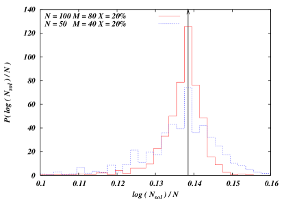
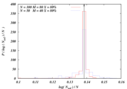
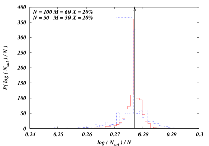
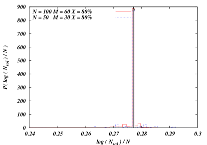
Figure 2: Histograms of the exhaustive algorithm estimates measured on $10000$ samples of $N=50$ (red boxes) and $N=100$ (blue boxes) for four different choices of $\alpha\in\{0.6,0.8\}$ and $X\in\{20\%,80\%\}$ expressed as a percentage. The black arrow is the numerical estimate using BP, that agrees perfectly with the theoretical value $\sigma=(1-\alpha)\ln 2$.

In Fig. (2) we display the frequency distribution of $\ln\mathcal{N}_{sol}$ for $10000$ samples at different values of $\alpha$ and $X$. Comparing these histograms one can observe that

• The most probable value of $P(s=\ln(\mathcal{N}_{sol})/N)$ depends strongly on $\alpha$ and only mildly on $X$.

• The distributions at increasing $N$ seem to peak around the value $s=(1-\alpha)\ln 2$.

4.2 Magnetization

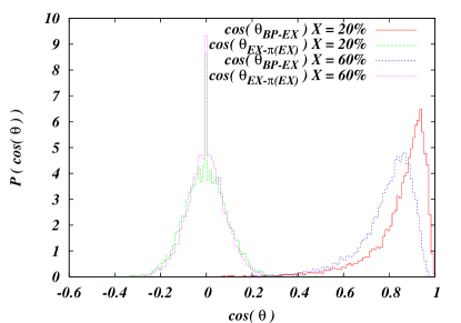
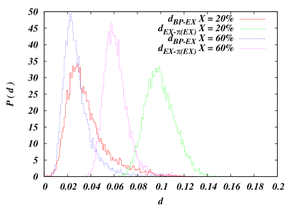
Figure 3: Histogram of $\cos(\theta_{BP-EX})$ compared with the reference histogram of $\cos(\theta_{EX-\pi(EX)})$ (left panel). In the right panel we display the histogram of both $d_{BP-EX}$ and $d_{EX-\pi(EX)}$. Measurement are done at $N=100$ $M=90$ and a percentage of XOR functions of $X=20\%,60\%$ over an ensemble of $10^{4}$ samples.

So far we have analyzed the behavior of the entropy alone. Although the entropy is very well predicted by BP, this is not always the case of the single variables marginal probabilities $P_{i}(x_{i})$ These quantities are of extreme importance in any decimation procedure that is expected to find a specific fixed point via BP. Necessary condition for any decimation procedure to be effective is, for each non pathological sample, a strong positive correlation between magnetization vectors ${\vec{m}}^{BP}$ and ${\vec{m}}^{EX}$, $N$-dimensional vectors whose $i$-th component represents the magnetization of each variable $x_{i}$ defined as

$$m^{BP/EX}_{i}=P_{i}^{BP/EX}(1)-P_{i}^{BP/EX}(0)\,\,\,,$$ (7)

where $P_{i}^{EX}(x)=P_{i}^{true}(x)=\mathcal{N}_{sol}(x_{i}=x)/\mathcal{N}_{sol}$. In order to assess this point, we define two global parameters testing respectively:

• the probability distribution of the relative angular overlap of the two magnetization vectors in the $N$ dimensional space, and

• the probability distribution of relative magnetization euclidean distances.

For each sample, the first overlap parameter is defined $\cos(\theta_{BP})$, i.e as the cosine of the angle between the exhaustive and BP magnetization vectors:

$$\cos(\theta_{BP-EX})\equiv\frac{\vec{m}^{BP}\cdot\vec{m}^{EX}}{|{m}^{BP}|\,\,|\vec{m}^{EX}|}\,\,.$$ (8)

The second is defined as the euclidean distance between non normalized magnetizations:

$$d_{BP-EX}=\frac{1}{N}\sqrt{\sum_{i=1}^{N}\left(m^{BP}_{i}-m^{EX}_{i}\right)^{2}}$$ (9)

In both cases the predictions have been tested against a null hypothesis. In the null hypothesis, random magnetization vectors are extracted in the following way: for each sample ${\vec{m}}^{\pi(EX)}$ is a random permutation of the components of ${\vec{m}}^{EX}$, so that $m^{\pi(EX)}_{i}\equiv m^{EX}_{\pi(i)}$ where $\pi(i)$ is a random permutation of the ordered set $\{1,\dots,N\}$. The quantities $\cos(\theta_{EX-\pi(EX)})$ and $d_{EX-\pi(EX)}$ are then calculated substituting ${\vec{m}}^{\pi(EX)}$ to ${\vec{m}}^{BP}$ in eqs.(8) and (9). Distributions of the overlaps over the sample populations are plotted in figure 3. The results show a strong correlation between the true and the predicted magnetization vector distributions.

4.3 Solutions overlap

It has been indicated in [10, 11] that in this model the entropy is analytic in all the phase diagram, while the organization of the fixed points undergoes a sudden reorganization at some $\alpha_{d}(X)$:

• At $\alpha<\alpha_{d}(X)$ all solutions are in a single cluster, i.e. any pair of solution is connected by a path via other solutions, where in each step only a finite number of variables can be changed.

• At $\alpha>\alpha_{d}(X)$ The space of solutions spontaneously breaks into an exponential number of macroscopically separated clusters of fixed points. Their number, or more precisely its normalized logarithm, is called complexity. It is a first-order phase transition.

This behavior is characterized by the appearance of a non-trivial structure of the space of solutions. In other words the fixed points, rather than being uniformly scattered over the $N$-dimensional hypercube, start to organize themselves in clusters, with a well defined intra-cluster and inter-cluster overlap. Nevertheless, by means of the exhaustive enumeration technique introduced above, one can easily write down all the solutions for a given sample and hence calculate all the ${\cal N}_{\mathrm{sol}}({\cal N}_{\mathrm{sol}}-1)/2$ overlaps, defined in a standard way as $q^{ab}=\frac{1}{N}\sum_{i=1}^{N}\sigma^{a}_{i}\sigma^{b}_{i}$. Note that we are using spin variables here $\sigma_{i}=-1+2{x_{i}}$, and $a,b$ indicates two distinct solutions. The distribution of the overlaps for two sizes and three different choices of $X$ are shown in figure 4. We choose a value far apart form the clustering transition line (no XOR functions), a value in the vicinity of the transition line ($50\%$ of XOR functions) and a value deep inside the clustered phase ($100\%$ of XOR functions).

Figure 4: Distribution of the overlaps for 10000 samples at $\alpha=0.93$. $X=0$ (left panel), $X=0.5$ (central panel), $X=1$ (right panel), for $N=50$ (thin line) and $N=100$ (thick line).

It is clear that as one moves from the unclustered to the clustered phase (which at fixed $\alpha$ is equivalent to increasing $X$), the distribution changes from a broad shape to a two-peaked one. However, this two-peaked pattern is just a finite size effect, as it seems to be indicated by the reduction of the weight of the right peak of the $P(q)$ from $N=50$ to $N=100$ shown in the left panel of figure 4. As the number of clusters is exponential in the system size, the probability of extracting two random solutions from the same cluster is negligibly small even for moderate sizes.

This phenomenon can be understood by the following qualitative argument: let us suppose that the number of clusters as well as the size of each single cluster are exponential in the system size. Let us further suppose that the distribution of cluster sizes is strongly peaked around a single value, ${\cal N}_{\mathrm{sol-in-cl}}$ (less stringent conditions can be found, together with pathological cases where those conditions do not hold, but a complete treatment would go beyond the scope of present work). In a completely clustered phase the weight contribution of the intra-cluster overlap will then be proportional to ${\cal N}_{\mathrm{cl}}{\cal N}^{2}_{\mathrm{sol-in-cl}}$ where ${\cal N}_{\mathrm{cl}}$ is the number of clusters. On the other hand, the contribution to the inter-cluster overlap is proportional to ${\cal N}^{2}_{\mathrm{cl}}{\cal N}^{2}_{\mathrm{sol-in-cl}}$ (i.e. all couple of solutions except those in the same clusters). If ${\cal N}_{\mathrm{cl}}$ is exponential in $N$, the intra-cluster contribution will be negligible with respect to the inter-cluster one in the thermodynamic limit.

5 Some considerations on the validity of the annealed approximation

In this section we will show that the logarithm of the number of solutions (i.e. the entropy) of our model of BNs computed within the annealed approximation scheme agrees with the numerical estimate for the entropy we performed by exhaustive enumeration and by the numerical solution of the BP equations on single sample.

This feature allows us to make some conjectures, and check whether the annealed approximation is exact in the $N\to\infty$ limit. We will show that the variance of $P(\mathcal{N}_{sol})$ as well as all higher moments are proportional to $2^{(1-\alpha)N}$ in the large $N$ limit, with a proportionality constant depending only on $\alpha$ and $X$. This implies that a non zero contribution to the entropy is given at the leading order only by the external regulating variables, in accordance with results obtained in [10, 11]. However, we will also show how, in the general case of $X<1$, the proportionality constants are different from one and greater than it, not ensuring the exactness of the annealed result, albeit replica results given in [10, 11] are a strong hint in that direction.

Moreover, we will see that in the thermodynamic limit:

$$\frac{\langle\mathcal{N}^{2}_{sol}\rangle}{\langle\mathcal{N}_{sol}\rangle^{2}}\equiv C(\alpha,X)$$ (10)

where $C(\alpha,X)$ is a constant independent of $N$. Only in the case of pure XOR classes ($X=1$), it is possible to show that the proportionality constant is exactly $1$ the large $N$ limit for any order moment and any value of $\alpha$, implying that the annealed approximation is exact.

Let’s consider a distribution of positive random variables $Z_{i}$. As we are interested in the relation between the quenched entropy and the annealed approximation, we want to investigate the relation between $\langle\ln Z\rangle$ and $\ln\langle Z\rangle$, where $\langle\phantom{Z}\rangle$ identifies here the average over the distribution of $Z_{i}$. We can write:

$$\langle\ln Z\rangle=\ln\langle Z\rangle+\langle\ln\frac{Z}{\langle Z\rangle}\rangle=\ln\langle Z\rangle+\sum_{i=2}^{\infty}\frac{(-1)^{i+1}}{i}\langle\Big{(}\frac{Z-\langle Z\rangle}{\langle Z\rangle}\Big{)}^{i}\rangle$$ (11)

where we have expressed the quenched entropy in term of the annealed one plus a series of the moments of the distribution. In our case we take $Z=\mathcal{N}_{sol}$. In cases where the sum of the series of moments is finite or for any $X$ and $\alpha$ diverges as a function $f(N)$ of the size of the graph such that $f(N)/N\to 0$, then the quenched and the annealed entropies coincide. We will show that this is the case at least for the second order moment. It is important to state, however, that the previous series expansion is valid only if $0<Z/\langle Z\rangle\leq 2$, and that averaging the resulting series term by term is possible only if the sum can be taken out of the integral which defines the average.

These conditions are not always met in our model, and in particular we expect the existence of a certain range of $X$ and $\alpha$ values beyond which the conditions are not necessarily satisfied. In particular we will also show that in the thermodynamic limit

$$\lim_{X\to 0}\lim_{\alpha\to 1}C(\alpha,X)=\infty$$ (12)

However this will not necessarily undermine the validity of the annealed calculation.

Under the hypothesis of equation (10), and thanks to a straightforward implementation of the Tschebichev inequality, one can easily show that, (see A.2)

$$\mbox{Pr}(\mathcal{N}_{sol}>\langle\mathcal{N}_{sol}\rangle)\leq 2^{-N\gamma}C(\alpha,X)$$ (13)

where $\gamma$ is a positive constant. This implies that, in the thermodynamic limit, the probability distribution of the number of solutions has support in the interval $(0,\langle\mathcal{N}_{sol}\rangle)$. Unfortunately in order to take under control also the left tail of the distribution one should compute moments of the type $\langle\mathcal{N}_{sol}^{n}\rangle$ with $0<n<1$, which is, as indicated in A.3, a rather complicated task.

5.1 General calculation of $\langle\mathcal{N}_{sol}\rangle$

Given a probability distribution of classes of Boolean functions $\pi(f)$, drawn independently, where $f$ is a generic Boolean function of $K=2$ inputs, and given a value of $\alpha\in[0,1]$ one can write

$$\langle\mathcal{N}_{sol}\rangle=\sum_{\vec{x}}\langle\prod_{m=1}^{M\sim\alpha N}\langle\delta(1;x_{0,m}f(x_{1,m},x_{2,m}))\rangle_{\pi(f)}\rangle_{\cal{G}}$$ (14)

where the external average is over the graph ensemble, while the internal one is over $\pi(f)$. Note that for the XOR class $f(x_{1},x_{2})=\epsilon x_{1}x_{2}$, while for the AND-OR class $f(x_{1},x_{2})=\epsilon_{0}/(2(\epsilon_{1}x_{1}\epsilon_{2}x_{2}+\epsilon_{1}x_{1}+\epsilon_{2}x_{2}-1))$, with $\epsilon_{i}\in\{\pm 1\}$ with a chosen probability and $X\in[0,1]$. The variables $\{x_{i}\}\in\{\pm 1\}^{N}$. Averaging over the values of $\{\epsilon_{i}\}_{i=0,1,2}$ and $X$ is therefore equivalent of averaging over the $\pi(f)$. In particular, in the case of flat classes distribution, which is the object of the present work, one has $prob(\epsilon)=(\delta(\epsilon-1)+\delta(\epsilon+1))/2$. Therefore:

$$\langle\mathcal{N}_{sol}\rangle=\sum_{\vec{x}}\langle\prod_{m=1}^{M\sim\alpha N}\langle\delta(1;x_{0,m}f(x_{1,m},x_{2,m}))\rangle_{\{\epsilon_{i}\},X}\rangle_{\cal{G}}$$ (15)

Let us now define $N_{o}=\alpha N$ regulated variables and $N_{i}=(1-\alpha)N$ external inputs (including the $(1-\alpha)e^{-2\alpha}$ isolated nodes). Assuming the input variables are extracted randomly and independently on each of the $N_{o}$ clauses; one can write

$$\langle\mathcal{N}_{sol}\rangle = \sum_{N^{+}_{o},N^{+}_{i}=0}^{N_{o},N_{i}}{N_{o}\choose N^{+}_{o}}{N_{i}\choose N^{+}_{i}}$$ (16)

$$\left[{\cal P}(++|+)g(+++)+{\cal P}(+-|+)g(+-+)+\right.$$

$$\left.{\cal P}(-+|+)g(-++)+{\cal P}(--|+)g(--+)\right]^{N^{+}_{o}}$$

$$\left[{\cal P}(++|-)g(++-)+{\cal P}(+-|-)g(+--)+\right.$$

$$\left.{\cal P}(-+|-)g(-+-)+{\cal P}(--|-)g(---)\right]^{N_{o}-N^{+}_{o}}$$

where ${\cal P}(\rho\sigma|\tau)$ is the probability of drawing two inputs of sign $\rho$ and $\sigma$ given the fact that one is looking at a clause with output variable sign $\tau$, and $g(\rho\sigma\tau)$ is the value of the function node $\delta(1;\tau f(\rho,\sigma))$ times the probability of extracting a certain Boolean function type $f$. In the case of uniform $\pi(f)$, ${\cal P}(\rho\sigma|\tau)g(\rho\sigma\tau)$ is trivially $1/8$ $\forall$ signs triplet, leading to $\langle\mathcal{N}_{sol}\rangle=2^{(1-\alpha)N}$ identically.

For a different distribution this is in general not the case. As a title of example, in the case of a mixture of pure XOR and AND functions, without any literal negation, $\pi(f)=X\delta(f;f_{\oplus})+(1-X)\delta(f;f_{\wedge})$ and eq.(16) reads

$$\langle\mathcal{N}_{sol}\rangle = \sum_{N^{+}_{o},N^{+}_{i}=0}^{N_{o},N_{i}}{N_{o}\choose N^{+}_{o}}{N_{i}\choose N^{+}_{i}}\cdot$$ (17)

$$\left[\frac{2X(N-N^{+})(N^{+}-1)}{(N-1)(N-2)}+(1-X)\frac{(N^{+}-1)(N^{+}-2)}{(N-1)(N-2)}\right]^{N^{+}_{o}}\cdot$$

$$\left[X\frac{N^{+}(N^{+}-1)}{(N-1)(N-2)}+\frac{(N-N^{+}-1)(N-N^{+}-2)}{(N-1)(N-2)}\right.$$

$$+\left.2(1-X)\frac{N^{+}(N-N^{+}-1)}{(N-1)(N-2)}\right]^{N_{o}-N^{+}_{o}}$$

Leading order terms can be computed following a calculation identical to the one shown below for the second moment, and will be omitted here.

5.2 General calculation of $\langle\mathcal{N}^{2}_{sol}\rangle$

For the second moment:

$$\langle\mathcal{N}^{2}_{sol}\rangle=\sum_{\vec{x},\vec{y}}\langle\prod_{m=1}^{M\sim\alpha N}\langle\delta(1;x_{0,m}f(x_{1,m},x_{2,m}))\delta(1;y_{0,m}f(y_{1,m},y_{2,m}))\rangle_{\{\epsilon_{i}\},X}\rangle_{\cal{G}}$$ (18)

Averaging uniformly over the function types one obtains

$$\langle\mathcal{N}^{2}_{sol}\rangle=\sum_{\vec{x}}\langle\prod_{m=1}^{M\sim\alpha N}\mathcal{G}^{(2)}(X;x_{0,m},x_{1,m},x_{2,m})\rangle_{\cal{G}}$$ (19)

with

$$\mathcal{G}^{(2)}(X;x_{0},x_{1},x_{2})=\frac{X}{2}(1+x_{0}x_{1}x_{2})+\frac{1-X}{2}((1+x_{1}+x_{2}+x_{1}x_{2})\frac{x_{0}}{4}+1)$$ (20)

Averages over different function types distributions are also possible, but beyond the scope of this work. Along the same line of arguments of the previous section, averaging over the Poissonian graph structure, one obtains

$$\langle\mathcal{N}^{2}_{sol}\rangle = \sum_{N^{+}_{o},N^{+}_{i}=0}^{N_{o},N_{i}}{N_{o}\choose N^{+}_{o}}{N_{i}\choose N^{+}_{i}}$$ (21)

$$\left[{\cal P}(++|+)g(X;+++)+{\cal P}(+-|+)g(X;+-+)+\right.$$

$$\left.{\cal P}(-+|+)g(X;-++)+{\cal P}(--|+)g(X;--+)\right]^{N^{+}_{o}}$$

$$\left[{\cal P}(++|-)g(X;++-)+{\cal P}(+-|-)g(X;+--)+\right.$$

$$\left.{\cal P}(-+|-)g(X;-+-)+{\cal P}(--|-)g(X;---)\right]^{N_{o}-N^{+}_{o}}$$

where $g(X;\rho\sigma\tau)$ is now the value of $\mathcal{G}^{(2)}$ given $X$ and the sign of the inputs. Equations (16) and (21) have an identical structure. This observation can be generalized and holds for any higher order momentum, changing the structure of the functions $g$. The details of the computation of the second moment are reported in A. At the leading order it turns out that:

$$\langle\mathcal{N}^{2}_{sol}\rangle\equiv I^{(2)}(\alpha,X)=2^{2(1-\alpha)N}C(\alpha,X)$$ (22)

The value of the multiplicative constant $C(\alpha,X)$ as a function of $X$ for increasing values of $\alpha$ is plotted in fig.(5).

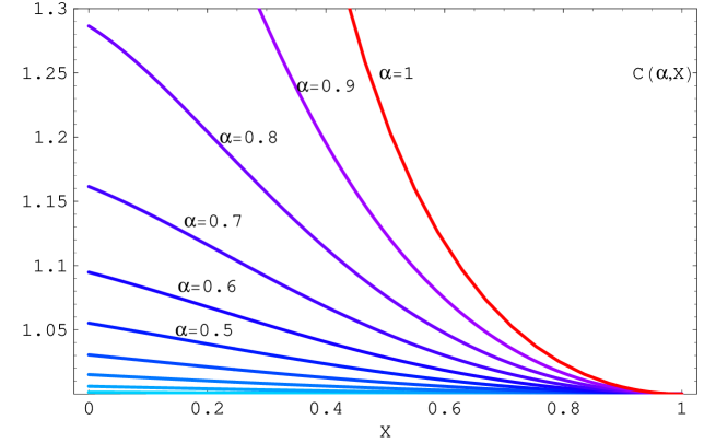
Figure 5: Plot of $C(\alpha,X)$ for the second moment of the distribution of the number of solutions in the large $N$ limit. The red uppermost line is the function $e^{(x-1)}/x$, diverging for $x\to 0$

Note that, unless in the pure XOR case, $C(\alpha,X)\neq 1$. This means that the analysis of the second order momentum is not enough to assess the theoretical validity of the annealed calculation of the entropy in the sense that the convergence of the logarithmic correction series is not ensured a priori. Moreover, whenever $C(\alpha,X)>1$, $\sigma^{2}_{{\cal N}_{sol}}=\langle\mathcal{N}^{2}_{sol}\rangle-\langle\mathcal{N}_{sol}\rangle^{2}\propto 2^{N(1-\alpha)}$.

5.2.1 The special case of $\alpha=1$

At $\alpha=1$ several simplifications in the computation of the second moment hold. Both the entropic contribution due to the external regulators, and the Kullback-Leibler terms are identically zero at the saddle point, as one can check from the saddle point equation for $\langle\mathcal{N}^{2}_{sol}\rangle$ presented in A. It turns out that the contribution to the saddle point includes also the term corresponding to the non-zero boundary term of integration. For the second moment in particular, one has to take into account the contribution of all terms around $N_{o}^{+}=N_{o}$.

Going back to eq.(21) and taking explicitly into account those terms, one obtains in the large $N$ limit

$$\langle\mathcal{N}^{2}_{sol}\rangle\to I^{(2)}(1,X)+\sum_{t=0}^{\infty}\frac{e^{-t(X+1)}(t-1)^{t}(X+1)^{t}}{t!}$$ (23)

where $I^{(2)}(1,X)=e^{(x-1)}/x$. The values of both contributions diverge for $X\to 0$. Analytic estimates suggest that the divergence goes as $\sqrt{N}$. In fig. 6 we display the numerical estimate of $\langle\mathcal{N}^{2}_{sol}\rangle$ obtained via exhaustive enumeration and the analytic estimate presented in eq. (21). The agreement is good, as it should be, since the computation of the second moment is exact, also for finite $N$.

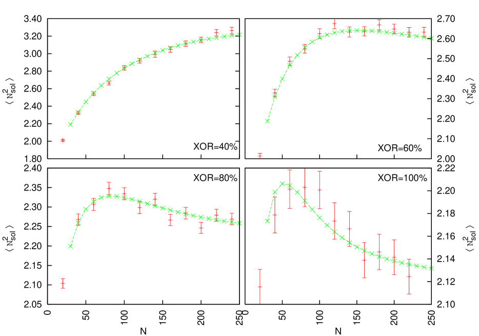
Figure 6: Second moment of the number of solutions distribution. Bars are computed by exhaustively counting the solutions for 100000 samples at $\alpha=1$, crosses by evaluating the analytical formula with Mathematica.

6 Conclusions

In this work we have investigated several aspects of the fixed points solutions set of a particular class of finite size diluted random Boolean networks with $K=2$ inputs per function. A search algorithm based on a state-of-the-art satisfiability solver was used to exhaustively enumerate fixed points up to moderate system sizes. For fixed system size ensembles the average number of solutions were plotted together with average fluctuations and with two additionally ad hoc defined order parameters indicating average distance between solutions within the fixed points set. A throughout comparison of the exact results with those given by the heuristic Belief Propagation algorithm was done in order to assess the performance of BP for small size samples whose network structure significantly deviates from tree-like. BP was shown to perform significantly well in the prediction of the correct number of solutions even in small sizes cases. BP seems to loose its predicting power in the calculation of single Boolean variables marginals at the fixed points; still it was shown to retain a significant correlation with exact results in the global spatial arrangements of the solutions. Furthermore, the analytical results closing the paper, together with their agreement with exact enumeration results, give a strong hint on the exactness of the annealed calculation of the entropy as well as the high order moments of the probability distribution of the number of solutions.

7 Acknowledgments

We are happy to acknowledge Martin Weigt for his suggestions about the computation of the first and second moment. We want also to thank Matteo Marsili, and Riccardo Zecchina, for many interesting discussions.

Appendix A The computation of the moments of $P(\mathcal{N}_{sol})$

We first present the details of the computations of the second moment and we will then give some hints on the structure of the generic $n^{th}$ moment.

A.1 The second order momentum

With respect to $\langle\mathcal{N}^{2}_{sol}\rangle$, if we keep only the leading order terms in eq.(21), the sums can be approximated by the following integral, where the exponent is given by the entropy contribution of the external variables plus a Kullback-Leibler distance term vanishing at the saddle point:

$$\langle\mathcal{N}^{2}_{sol}\rangle=I^{(2)}(\alpha,X) = 2^{(1-\alpha)N}\int_{0}^{1}\int_{0}^{1}db_{o}^{+}db_{i}^{+}K(\alpha,X,b_{o}^{+},b_{i}^{+})e^{N{\cal F}[\alpha,X,b_{o}^{+},b_{i}^{+}]}$$

$$K(\alpha,X,b_{o}^{+},b_{i}^{+}) = \frac{\sqrt{\alpha(1-\alpha)}}{\sqrt{b_{o}^{+}b_{i}^{+}(1-b_{o}^{+})(1-b_{i}^{+})}}e^{\alpha B(\alpha,X,b_{o}^{+},b_{i}^{+})}$$

$${\cal F}[\alpha,X,b_{o}^{+},b_{i}^{+}] = (1-\alpha)H(b_{i}^{+})+\alpha D_{KL}(b_{o}^{+}|G(\alpha,X,b_{o}^{+},b_{i}^{+}))$$

$$B(\alpha,X,b_{o}^{+},b_{i}^{+}) = 3-\frac{3b^{+}b_{o}^{+}+(1-X)(1-b^{+})b_{o}^{+}+(1+X)(1-b^{+})b_{o}^{+}/2}{(b^{+})^{2}+(1-X)(1-b^{+})b_{o}^{+}+(1+X)(1-b^{+})^{2}/2}$$

$$- \frac{(1+X)(b^{+}(1-b_{o}^{+})+3(1-X)(1-b^{+})(1-b_{o}^{+})/2}{1-(b^{+})^{2}+(1-X)(1-b^{+})b_{o}^{+}-(1+X)(1-b^{+})^{2}/2}$$

$$H(x) = -x\log(x)-(1-x)\log(1-x)$$

$$D_{KL}(x|y) = x\log\left(\frac{y}{x}\right)+(1-x)\log\left(\frac{1-y}{1-x}\right)$$

$$G(\alpha,X,b_{o}^{+},b_{i}^{+}) = (b^{+})^{2}+(1-X)b^{+}(1-b^{+})+\frac{1+X}{2}(1-b^{+})^{2}$$

$$b^{+}(\alpha,b_{o}^{+},b_{i}^{+}) = \alpha b_{o}^{+}+(1-\alpha)b_{i}^{+}$$

where $b_{o}^{+}=N_{o}^{+}/N_{o}$ and $b_{i}^{+}=N_{i}^{+}/N_{o}$. The value of the Integral $I^{(2)}(\alpha,X)$ can be calculated at the saddle point

$${\tilde{b}}_{i}^{+} = \frac{1}{2}$$ (24)

$${\tilde{b}}_{o}^{+} = G(\alpha,X,{\tilde{b}}_{o}^{+},{\tilde{b}}_{i}^{+})$$

$$= \frac{2-\alpha(1-\alpha)+\alpha X(1+3\alpha)-2\sqrt{1-\alpha(1-X)+\alpha^{2}X(X-1)}}{2\alpha^{2}(1+3X)}$$

Finite $N$ corrections can be in principle computed extending the calculation of $K$ to higher orders in ${\cal O}(1/N)$, and performing an asymptotic expansion around the saddle point. Whenever $\alpha<1$ and $X>0$ it can be seen that the condition (A.1) finds the only maximum ${\cal F}$, which lies within the integration interval.

A.2 An upper bound on the number of solutions

In this subsection we will show that in the thermodynamic limit the support of $P(\mathcal{N}_{sol})$ is contained in the interval $(0,\langle\mathcal{N}_{sol}\rangle)$, using, as we have already shown in the previous section, that:

$$\langle\mathcal{N}_{sol}\rangle = 2^{(1-\alpha)N}$$

$$\langle\mathcal{N}^{2}_{sol}\rangle = 2^{2(1-\alpha)N}C(\alpha,X)$$ (26)

where $C(\alpha,X)$ is a constant independent from $N$. The one-tailed Chebyshev inequality states that:

$$\mbox{Pr}\left(\mathcal{N}_{sol}>\langle\mathcal{N}_{sol}\rangle\right)\leq\frac{\langle\mathcal{N}^{2}_{sol}\rangle}{(\mathcal{N}_{sol}-\langle\mathcal{N}_{sol}\rangle)^{2}}\,\,\,\,.$$ (27)

Under the condition $\mathcal{N}_{sol}>\langle\mathcal{N}_{sol}\rangle$ we can express $\mathcal{N}_{sol}=2^{N\Sigma^{\prime}}$ where $\Sigma^{\prime}>(1-\alpha)$. Inserting eqs. (26) into eq. (27) we get:

$$\mbox{Pr}\left(\mathcal{N}_{sol}>\langle\mathcal{N}_{sol}\rangle\right) \leq \frac{2^{2(1-\alpha)N}C(\alpha,X)}{2^{2N\Sigma^{\prime}}(1-2^{N(1-\alpha-\Sigma^{\prime})})}\leq 2^{2N(1-\alpha-\Sigma^{\prime})}C(\alpha,X)$$ (28)

$$= 2^{-N\gamma}C(\alpha,X)\,\,\,\,,$$

where $\gamma$ is a positive constant making the right tail of the $P(\mathcal{N}_{sol})$ distribution (i.e. for values of $\mathcal{N}_{sol}>\langle\mathcal{N}_{sol}\rangle$) exponentially small in $N$, as we wanted to show. Indeed, this simple result is enough to imply that no contribution to the entropy is given by instances whose number of solutions is larger than the annealed value. The support of the probability distribution of entropy values $P(S)$ must be therefore $[0,S_{annealed}]$. In order to prove that also smaller values do not take part of the support, one would need to calculate fractional order moments, as explained in the end of next section.

A.3 Higher order moments

For the general $n^{th}$ order momentum one can write, along the same line of reasoning:

$$\langle\mathcal{N}^{n}_{sol}\rangle = \sum_{\{N^{\sigma_{1}...\sigma_{n-1}}_{o}\}=0}^{N_{o}}\sum_{\{N^{\sigma_{1}...\sigma_{n-1}}_{i}\}=0}^{N_{i}}\frac{N_{o}!N_{i}!}{\prod_{\vec{\sigma}}N^{\sigma_{1}...\sigma_{n-1}}_{o}!N^{\sigma_{1}...\sigma_{n-1}}_{i}!}\cdot$$ (29)

$$\delta(N_{o};\alpha N)\delta(N_{i};(1-\alpha)N)\prod_{\vec{\sigma}}T(\vec{\sigma})\cdot$$

$$\delta(N_{o};\sum_{\vec{\sigma}}N^{\sigma_{1}...\sigma_{n-1}}_{o})\delta(N_{i};\sum_{\vec{\sigma}}N^{\sigma_{1}...\sigma_{n-1}}_{i})$$

with

$$T(\vec{\sigma}) = \left[\sum_{\vec{\sigma^{(1)}}}\sum_{\vec{\sigma^{(2)}}}{\cal P}(\sigma_{1}^{(1)}\sigma_{1}^{(2)},...,\sigma_{n-1}^{(1)}\sigma_{n-1}^{(2)}|\sigma_{1},...,\sigma_{n-1})\cdot\right.$$

$$\left.g(\sigma_{1}^{(1)}\sigma_{1}^{(2)},...,\sigma_{n-1}^{(1)}\sigma_{n-1}^{(2)}|\sigma_{1},...,\sigma_{n-1})\right]^{N^{\sigma_{1}...\sigma_{n-1}}_{o}}$$

where we are summing over all configurations overlaps with $N^{\sigma_{1}...\sigma_{n-1}}_{o}/N^{\sigma_{1}...\sigma_{n-1}}_{i}$ output/input variables of signs $\sigma_{1}...\sigma_{n-1}$, the ${\cal P}$ represent the probability of finding $n-1$ real replicas of an input variables couple in a given function, and $g$ the value of the $(n-1)^{th}$ averaged product of the replicated Boolean function.

As before, from the leading terms of eq.(LABEL:eeq7), one gets

$$\langle\mathcal{N}^{n}_{sol}\rangle \to I^{(n)}(\alpha,X)$$

$$I^{(n)}(\alpha,X) = 2^{(1-\alpha)N}\int_{0}^{1}\prod_{{\vec{\sigma}}}d\{b_{o}\}d\{b_{i}\}K^{(n)}(\alpha,X,\{b_{o},b_{i}\})e^{N{\cal F}^{(n)}[\alpha,X,\{b_{o},b_{i}\}]}$$

with

$${\cal F}^{(n)}[\alpha,X,\{b_{o},b_{i}\}] = (1-\alpha)H^{(n)}+\alpha D^{(n)}_{KL}(\{b_{o}\}|G^{(n)})$$

$$H^{(n)}(\alpha,X,\{b_{o},b_{i}\}) = \sum_{{\vec{\sigma}}}b_{i}^{\sigma_{1}...\sigma_{n-1}}\log(b_{i}^{\sigma_{1}...\sigma_{n-1}})$$

$$D^{(n)}_{KL}(\{b_{o}\}|G^{(n)}) = \sum_{{\vec{\sigma}}}b_{o}^{\sigma_{1}...\sigma{n-1}}\log\left(\frac{G^{(n)}}{b_{0}^{\sigma_{1}...\sigma{n-1}}}\right)$$ (32)

with $b_{o,i}^{\sigma_{1}...\sigma_{n-1}}=N_{o,i}^{\sigma_{1}...\sigma_{n-1}}/N_{o,i}$ and $\{b_{o,i}\}=\{b_{o,i}^{\sigma_{1},...,\sigma_{n-1}}\}_{\vec{\sigma}\in\{\pm 1\}^{n-1}}$ . The explicit form of functions $G^{(n)}$ and $K^{(n)}$ is not given here for brevity. Due to the general form of the exponent, the unique saddle point can always be computed as the one fulfilling conditions:

$${\tilde{b}}_{i}^{\sigma_{1}...\sigma_{n-1}} = \frac{1}{2^{n-1}}$$

$${\tilde{b}}_{o}^{\sigma_{1}...\sigma_{n-1}} = G^{(n)}(\alpha,X,\{{\tilde{b}}_{o}^{\sigma_{1}...\sigma_{n-1}}\},\{{\tilde{b}}_{i}^{\sigma_{1}...\sigma_{n-1}}\})$$ (33)

such that

$$I^{(n)}(\alpha,X)=2^{n(1-\alpha)N}C^{(n)}(\alpha,X)=\langle\mathcal{N}_{sol}\rangle^{n}C^{(n)}(\alpha,X)$$ (34)

Unfortunately, the explicit calculation of the function $C^{(n)}(\alpha,X)$ for all $n$ seems not to be easily accessible. Let us just finally note that one could prove that the distribution of the logarithm of the number of solutions $P(S)$ tends to $\delta(S-S_{\mathrm{annealed}})$ in the large $N$ one by showing that:

$$\lim_{n\rightarrow 0}\lim_{N\rightarrow\infty}C^{(n)}(\alpha,X)=1$$ (35)

which seems reasonable given the structure of eqs. (32, 33, 34), and the numerical result displayed in section 4.1, but, again, too difficult to be shown explicitly.

References

- [1] S. Kauffman, Journal of Theoretical Biology 22, 437 (1969).
- [2] M. Aldana Gonzalez, S. Coppersmith, and L.P. Kadanoff in Perspectives and Problems in Nonlinear Science, Applied Matematical Science, Springer, (2003).
- [3] E. R. Dougherty, I. Shmulevich, J. Chen, Z. J. Wang, Eds., Genomic Signal Processing and Statistics, EURASIP, (2005).
- [4] S. Kauffman, The Origins of order, Oxford University Press, NY, (1993).
- [5] B. Samuelsson, C. Troein, Phys. Rev. Lett. 90, 098701 (2003).
- [6] U. Bastolla, G. Parisi PHYSICA D, 98, 1 (1997); J. Theoretical Biology, 187, 117, (1997).
- [7] F. Derrida, Y. Pomeau, Europhysics Letters 1, 45 (1986).
- [8] M. Mezard, G. Parisi, and R. Zecchina, Science 297, 812 (2002);
- [9] A. Hartmann, M. Weigt, “Phase Transitions in Combinatorial Optimization Problems”, Wiley-VCH, Berlin, (2005).
- [10] L. Correale, M. Leone, A. Pagnani, M. Weigt, R. Zecchina, Phys. Rev. Lett. 96, 018101 (2006).
- [11] L. Correale, M. Leone, A. Pagnani, M. Weigt, R. Zecchina, J. Stat. Mech., P03002 (2006).
- [12] S. Kauffman, C. Peterson, B. Samuelsson, and C. Troein, PNAS 100, 14796 (2003) and PNAS 101, 17102 (2004).
- [13] J.S. Yedidia, W.T. Freeman, Y. Weiss, in Advances in Neural Information Processing Systems, MIT press, 689 (2001).
- [14] F.R. Kschischang, B.J. Frey, H.A. Loeliger, IEEE Transactions on Information Theory, 47, 498, 2001.
- [15] A. Braunstein, M. Mézard, R. Zecchina, Random Structures and Algorithms 27 issue 2, 201 (2005).
- [16] http://www.satlib.org/solvers.html
- [17] R. J. Bayardo Jr. and R. C. Schrag. Using CSP look-back techniques to solve real world SAT instances. In Proc. of the 14th National Conf. on Artificial Intelligence, 203-208 (1997). http://www.bayardo.org/resources.html.