Spin transport in mesoscopic rings with inhomogeneous spin-orbit coupling

Abstract

We revisit the problem of electron transport through mesoscopic rings with spin-orbit (SO) interaction. In the well-known path-integral approach, the scattering states for a quasi-1D ring with quasi-1D leads can be expressed in terms of spinless electrons subject to a fictitious magnetic flux. We show that spin-dependent quantum-interference effects in small rings are strongest for spatially inhomogeneous SO interactions, in which case spin currents can be controlled by a small external magnetic field. Mesoscopic spin Hall effects in four-terminal rings can also be understood in terms of the fictitious magnetic flux.

I Introduction

The Aharonov-Bohm (AB) effect in quasi-one-dimensional (1D) ringsAharonov and Bohm (1959) and, more generally, the adiabaticBerry (1984) and nonadiabaticAharonov and Anandan (1987) Berry holonomies manifest nontrivial quantum topology. Recently, this has attracted much attention in mesoscopic transport, exotic particle statistics, and topological quantum computation. The interest in spintronics, which aims to inject, manipulate, and detect electron spins in electronic devices, has also led many authors to revisit geometric aspects of transport in semiconductors with spin-orbit (SO) coupling,Meir et al. (1989); Mathur and Stone (1992); Qian and Su (1994) mainly focusing on variants of the Aharonov-Casher (AC) effect.Aharonov and Casher (1984) The AC effect in planar structures with Rashba SO coupling was recently observed in single rings König et al. (2006) and ring arrays.Koga et al. (2006)

Existing studies of AC related effects in mesoscopic rings focus on spatially homogeneous SO coupling.Nitta et al. (1999); Souma and Nikolić (2005); König et al. (2006) However, we will show that quantum-interference effects in mesoscopic rings are stronger for spatially varying SO interactions in systems smaller than the SO precession length (typically 1 $\mu$m or longer in InAs-based heterostructures).Brouwer et al. (2002); Stern (1992) An inhomogeneous SO interaction can be experimentally realized by electrostatic gates in semiconductor nanostructures, as sketched in Fig. 1. Electrostatic gates partially covering a planar ring induce an inhomogeneous macroscopic electric field perpendicular to the ring, influencing the electron motion via the spin-orbit interaction. Such an inhomogeneous SO coupling gives rise to a fictitious magnetic field with $SU(2)$ symmetry. In the weak SO limit, the corresponding fictitious flux dominates the geometric AC phase. Spin and charge flow in mesoscopic rings can therefore be manipulated by a combination of spatially varying SO interactions, which induces fictitious magnetic fields, and weak external magnetic fields.

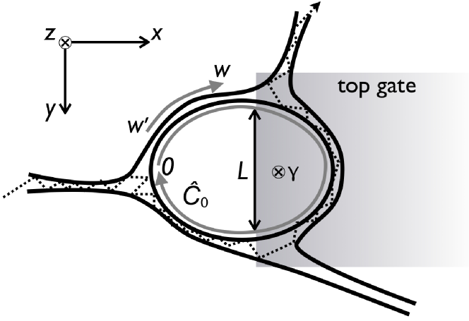
Figure 1: A multiterminal quasi-1D ring in the $xy$ plane. A spatially inhomogeneous SO interaction is induced by the top gate. $\hat{C}_{0}$ defines SO-induced spin rotation in a full clockwise loop around the ring with respect to a chosen reference point $0$. The dotted line shows a particle trajectory between two leads with a winding number $n=-1$.

Quantum-interference effects due to SO interactions linear in momentum in quasi-1D structures are most conveniently studied with path integrals, see e.g., Ref. Chakravarty and Schmid, 1986. This formulation gives a clear physical picture of geometric aspects of spin transport in mesoscopic rings, allowing one to complement and generalize recent discussions on AC phases in multiterminal rings.Nitta et al. (1999); Souma and Nikolić (2005); König et al. (2006) The path-integral approach recasts spin transport with arbitrary scalar disorder and smooth SO coupling in terms of conventional AB physics for spinless particles and purely geometric $SU(2)$ phase factors, and is valid, e.g., for both diffusive and ballistic transport. Not being limited to two-terminal configurations, we will also see that the spin Hall effect in four-terminal rings, such as that shown in Fig. 2, can be mapped onto the usual spinless Hall effect.

II Model

We consider a ring in the $xy$ plane as shown in Fig. 1. The electronic states are determined by the Hamiltonian

$$\hat{H}=\frac{1}{2m}[-i\hbar\boldsymbol{\nabla}+(e/c)\mathbf{\hat{A}}(\mathbf{r})]^{2}-eV(\mathbf{r})\,,$$ (1)

where $m$ is the effective mass, $-e$ electron charge, and the scalar potential $V(\mathbf{r})$ includes applied, gate, and disorder fields. Hats denote $2\times 2$ matrix structure in spin space for spin-$1/2$ particles. In the following, we will assume a vacuumlike SO coupling (although the arguments hold for any SO interaction linear in momentum, such as the Dresselhaus SO coupling,Dresselhaus (1955)) which can be described by the effective vector potential

$$\mathbf{\hat{A}}(\mathbf{r})=\mathbf{A}_{m}(\mathbf{r})+\lambda(\mathbf{r})\mathbf{E}_{\mathrm{eff}}(\mathbf{r})\times\boldsymbol{\hat{\sigma}}\,,$$ (2)

where $\mathbf{A}_{m}$ is the vector potential related to the applied magnetic field, $\mathbf{B}_{m}=\boldsymbol{\nabla}\times\mathbf{A}_{m}$ (disregarding Zeeman splitting), $\boldsymbol{\hat{\sigma}}$ is a vector of Pauli matrices, and $\lambda$ is a phenomenological material-dependent SO parameter (in vacuum, $\lambda=-\hbar/4mc$, but it is many orders of magnitude larger in narrow-gap semiconductors such as GaAs and, especially, InAs). $\mathbf{E}_{\mathrm{eff}}$ can consist of both the applied electric field and the macroscopic band-structure contribution due to the crystal fields. Note that the $\lambda^{2}$ term in the Hamiltonian (1) can be absorbed by a redefinition of $V(\mathbf{r})$, since $(\mathbf{E}\times\boldsymbol{\hat{\sigma}})^{2}=2E^{2}$. Electromagnetic $U(1)$ gauge invariance for the magnetic component of the effective vector potential $\mathbf{\hat{A}}$ gives rise to the AB effect and the $SU(2)$ gauge symmetry for the spin-dependent component causes the AC effect.Fröhlich and Studer (1993) It is useful to define an effective $2\times 2$ magnetic field,

$$\mathbf{\hat{B}}=\boldsymbol{\nabla}\times\mathbf{\hat{A}}=\mathbf{B}_{m}+\mathbf{\hat{B}}_{f}\,,$$ (3)

which includes the fictitious SO contribution $\mathbf{\hat{B}}_{f}$. Note that the fictitious $2\times 2$ magnetic field $\mathbf{\hat{B}}_{f}$ vanishes for a spatially homogeneous SO interaction.

For the Rashba SO coupling,Yu. I. Bychkov and Rashba (1984) $\mathbf{E}_{\rm eff}$ is along the $z$ direction, and, after including the magnitude of $\mathbf{E}_{\rm eff}$ into the coefficient $\lambda$, the fictitious field and the associated flux through the ring are given by

$$\mathbf{\hat{B}}_{f} =(\boldsymbol{\hat{\sigma}}\cdot\boldsymbol{\nabla}\lambda)\mathbf{z}\,,$$ (4)

$$\hat{\phi}_{f} =\int_{A}d^{2}r(\mathbf{z}\cdot\mathbf{\hat{B}}_{f})\,.$$ (5)

Diagonalization of this flux in spin space determines the spin quantization axis with corresponding fictitious magnetic fluxes of equal magnitude but opposite sign for spins up and down. For example, if $\lambda$ is induced by a top gate at $x>x_{0}$, with $\lambda(x>x_{0})=\lambda_{0}$ under the gate and vanishing outside of the gate, then $\hat{\phi}_{f}=\lambda_{0}L\hat{\sigma}_{x}$, where $L$ is the length of the top gate edge at $x=x_{0}$ overlapping the loop area, see Fig. 1. We may now naïvely conclude that the spin-up (down) transport is governed by the transport coefficients $g(\phi_{m}\pm\gamma\phi_{0})$, with the spin-quantization axis along the $x$ axis. This will be indeed justified below. $g(\phi)$ can denote any transport coefficients in two- or multiterminal configurations, e.g., the current response in one contact to voltages applied at two other contacts, as a function of the magnetic flux $\phi$ through the ring, in the absence of the SO coupling. $\phi_{m}$ is the physical magnetic field contribution to the flux, while $\gamma=\lambda_{0}L/\phi_{0}$ is the fictitious contribution due to the SO interaction, in units of the magnetic flux quantum $\phi_{0}=hc/e$. Keeping only linear in SO coupling $\gamma$ terms, the total conductance per spin equalsMeir et al. (1989)

$$g_{c}=\frac{1}{2}[g(\phi_{m}+\gamma\phi_{0})+g(\phi_{m}-\gamma\phi_{0})]\approx g(\phi_{m})\,,$$ (6)

while the spin conductance is

$$g_{s}=\frac{1}{2}[g(\phi_{m}+\gamma\phi_{0})-g(\phi_{m}-\gamma\phi_{0})]\approx\gamma\phi_{0}\partial_{\phi}g(\phi_{m})\,.$$ (7)

According to Eqs. (6) and (7), the magnetic flux $\phi_{m}$ through the ring can be used to modulate both spin and charge transport and the spin response is proportional to the SO coupling. Even such a simple setup, an electrostatic gate partially covering the ring and inducing inhomogeneous SO coupling, can thus exhibit nontrivial spintronic applications.

Note that the fictitious magnetic field (4) and the corresponding flux (5) are relevant only when we are interested in the linear in SO coupling effects. In particular, a homogeneous SO coupling $\lambda$ induces no fictitious field (4). Nevertheless, the noncommutative $2\times 2$ SO vector potential $\mathbf{\hat{A}}(\mathbf{r})$ does not allow a removal of the SO field by a gauge transformation altogether. The vanishing field (4) for homogeneous SO interactions suggests that the SO effects are manifested in transport properties at higher orders in the SO strength, as detailed in the following. In particular, even in the absence of a fictitious field $\mathbf{\hat{B}}_{f}$, there is in general a finite effective flux $\gamma$, which in the leading order is quadratic in the SO strength. Consequently, for a weak SO strength, inhomogeneous SO interactions are more effective than their homogeneous counterpart in generating spin-dependent transport effects. The relevant small parameter here is the fictitious magnetic flux $\gamma$, in units of $\phi_{0}$. In the above example, $\gamma=L/2l_{\rm so}$, where

$$l_{\rm so}=\frac{\phi_{0}}{2\lambda}=\frac{\pi\hbar^{2}}{\alpha m}$$ (8)

is the spin-precession length expressed in terms of the Rashba SO parameter $\alpha=e\hbar\lambda/cm$. Taking $\alpha=10^{-11}$ eV m (which is at the upper limit of typical values for InAs-based heterostructures Koga et al. (2006)) and $m=0.05m_{e}$, in terms of the free-electron mass $m_{e}$, we get $l_{\rm so}\approx 1/2$ $\mu$m. We thus conclude that linear in SO coupling effects will dominate in submicron systems if the SO profile is strongly inhomogeneous on the scale of the spin-precession length.

III Path-integral approach

For a more systematic study of topological properties for arbitrary SO strength, we express the evolution operator in terms of path integrals. To this end, we are interested in the $2\times 2$ propagator $\hat{K}(\mathbf{r},\mathbf{r}^{\prime};t)$ for the Schrödinger equation $i\hbar\partial_{t}\hat{\varphi}=\hat{H}\hat{\varphi}$, where $\hat{\varphi}(\mathbf{r},t)$ is the spinor column:Chakravarty and Schmid (1986)

$$\hat{K}(\mathbf{r},\mathbf{r}^{\prime};t)=T_{c}e^{-\frac{2\pi i}{\phi_{0}}\int_{c}d\mathbf{r}\lambda\left(\mathbf{E}_{\mathrm{eff}}\times\boldsymbol{\hat{\sigma}}\right)}\int\mathcal{D}[\mathbf{r}(t)]e^{\frac{i}{\hbar}S}\,.$$ (9)

Here, $\mathcal{D}[\mathbf{r}(t)]$ schematically denotes all trajectories in space-time connecting points $\mathbf{r}$ and $\mathbf{r}^{\prime}$ in time $t$, $S[\mathbf{r}(t)]$ is the corresponding classical action for spinless motion, and $T_{c}$ is the contour ordering operator that moves operators in the expanded exponential which are further along the contour to the left. The contour ordering is necessary for inhomogeneous effective fields $\mathbf{E}_{\mathrm{eff}}$, since the Pauli matrices do not commute. We now assume the potential $V(\mathbf{r})$ constrains the orbital motion within a narrow quasi-1D ring connected to several wires, see Fig. 1. Within each wire and the ring, electrons can scatter and undergo arbitrary orbital motion governed by the potential $V(\mathbf{r})$, but we disregard the net spin precession determined by $\mathbf{E}_{\mathrm{eff}}$ for the transverse motion within the quasi-1D channels, and focus on the phase accumulated during the propagation along the ring. This requires the characteristic SO precession length to be much longer than the wire widths, which is easily realized experimentally. The key observation, according to Eq. (9), is that the SO-induced phase is purely geometric and independent of how fast the electrons propagate.

In order to formally separate the geometric contribution to the propagator (9), we first need to make a convention for labeling quasi-1D paths connecting an arbitrary point $w^{\prime}$ in the system (either in the ring or the connected wires) to another point $w$. In the following, we suppress the transverse degrees of freedom along the connectors and the loop. The paths along the ring are classified according to the number of clockwise windings, $n$. We define the $n=0$ path to be the shortest clockwise path between the points $w^{\prime}$ and $w$. A finite positive (negative) $n$ corresponds to $n$ additional clockwise (counterclockwise) windings around the loop. The shortest clockwise path from $w^{\prime}$ to $w$ is shown in Fig. 1. In addition, we choose an arbitrary point in the loop [e.g., the contact between a wire and the ring, as in Fig. 1], denoted by $w=0$, to be the reference point. Let us denote the contour-ordered spin-rotation operator entering Eq. (9) for the $n$th path from $w^{\prime}$ to $w$ by $\exp[i\hat{C}_{n}(w,w^{\prime})]$, where $\hat{C}_{n}(w,w^{\prime})$ is a $2\times 2$ Hermitian matrix determined by $\mathbf{E}_{\mathrm{eff}}$ along the path. The eigenstates $\epsilon$ of the Hamiltonian (1) can now be found from the eigenvalue problem

$$i\hbar\int dw^{\prime}\sum_{n}e^{i\hat{C}_{n}(w,w^{\prime})}\partial_{t}K_{n}(w,w^{\prime};t)\hat{\varphi}(w^{\prime})=\epsilon\hat{\varphi}(w)$$ (10)

at $t=0$, where $K_{n}(w,w^{\prime};t)$ is the propagator for spinless electron motion. The spin-orbit interaction contributes only to the path-dependent $SU(2)$ geometric prefactor. The eigenvalue problem (10) can be diagonalized in spin space, after we make several definitions: Let $\hat{C}_{0}=\hat{C}_{0}(0,0^{+})$, where $0^{+}$ is a point slightly clockwise offset from $0$, so that $\hat{C}_{0}$ corresponds to one full cycle with respect to $w=0$. $e^{i\hat{C}_{0}}$ is diagonalized by a unitary transformation:

$$\hat{U}^{\dagger}e^{i\hat{C}_{0}}\hat{U}=\mathrm{diag}\{e^{\mp 2\pi i\gamma}\}\,,$$ (11)

with a unique $\gamma$ in the range $0\leq\gamma<1$. We next introduce a fictitious vector potential $\mathbf{A}_{\gamma}(\mathbf{r})=-\mathbf{A}_{-\gamma}(\mathbf{r})$ corresponding to the magnetic flux $\pm\gamma$ (in units of $\phi_{0}$), respectively, through the loop, see Fig. 1, but in an otherwise arbitrary gauge. Finally,

$$\theta(w,w^{\prime})=\frac{2\pi}{\gamma\phi_{0}}\int_{w^{\prime}}^{w}d\mathbf{q}\cdot\mathbf{A}_{\gamma}$$ (12)

is a line integral along the $n=0$ path from $w^{\prime}$ to $w$ around the loop, so that $\theta(w,w+0^{+})=2\pi$ and $\theta(w,w-0^{+})=0$ for points $w$ inside the ring. We are now ready to make the transformation:

$$\hat{\varphi}(w)=e^{i\hat{C}_{0}(w,0)}\hat{U}\mathrm{diag}\{e^{\pm i\gamma\theta(w,0)}\}\hat{\varphi}^{\prime}(w)\,.$$ (13)

Note that this is a smooth transformation when the SO interaction and the magnetic field are smooth. Straightforward manipulations show that substituting Eq. (13) into Eq. (10) diagonalizes the eigenvalue problem for two spin species:

$$\mathrm{diag}\{H_{\pm\gamma}\}\hat{\varphi}^{\prime}=\epsilon\hat{\varphi}^{\prime}\,,$$ (14)

where $H_{\pm\gamma}$ is the Hamiltonian with the potential $V(\mathbf{r})$, vector potential $\mathbf{A}_{m}(\mathbf{r})$ due to the external magnetic field, but with the SO coupling replaced by the additional spin-dependent fictitious vector potential $\mathbf{A}_{\pm\gamma}(\mathbf{r})$. The eigenvalues and eigenstates of our original Hamiltonian (1) can thus be expressed in terms of the solution of the simpler problem, Eq. (14), describing spinless electron experiencing a magnetic flux, which was discussed extensively in various contexts. The spin texture corresponding to the SO coupling is then added by a purely geometric unitary transformation (13). SO interactions linear in momentum thus do not add any complexity to the electronic structures of general multiterminal quasi-1D rings. We thus remark that many of the results discussed in Ref. Nitta et al., 1999 can be readily obtained after solving the problem of magnetotransport for spinless electrons and then making the transformation (13) (valid for arbitrarily strong SO coupling) in order to get detailed information about spin as well as charge transport.

We can now return to justify the use of the fictitious magnetic field (4) for inhomogeneous SO coupling in the discussion leading to Eqs. (6) and (7). In the weak SO limit, to linear order in $\lambda$,

$$e^{i\hat{C}_{0}}\approx e^{-2\pi i\frac{\hat{\phi}_{f}}{\phi_{0}}}\,,$$ (15)

where $\hat{\phi}_{f}$ is given by Eq. (5). Using the Hausdorff formula,

$$e^{\hat{A}}e^{\hat{B}}=e^{\hat{A}+\hat{B}+\frac{1}{2}[\hat{A},\hat{B}]+...}\,,$$ (16)

it is clear that corrections to the approximation (15) are quadratic in $\lambda$, corresponding to non-commuting spin rotations along the loop contour, and can be disregarded for systems smaller than the spin-precession length $l_{\rm so}$. The spin transport problem thus reduces to the AB effect for two spin species along the quantization axis determined by $\hat{\phi}_{f}$, with opposite fictitious fluxes. Since this quantum-interference effect is linear in the SO strength, this regime can become useful in practice when a weak SO coupling is modulated by external electrostatic gates. We should note here that in the spirit of the approximation, i.e., for the spin-transport properties linear in the SO strength, the additional spin transformation determined by $\hat{C}_{0}(r,0)$ in Eq. (13), which rotates spins at position $\mathbf{r}$ by an angle linear in the SO coupling, can be disregarded, as well as ambiguities in defining spin currents and spin conductances in the leads with a finite SO coupling $\lambda$.

IV Four-terminal longitudinal and Hall spin currents

After the general discussion of Sec. III, let us now consider a specific example that illustrates how the theory can be applied in practice to i) enhance spin-dependent effects and ii) control the size and direction of the induced spin currents and accumulations. We will analyze spin-dependent transport through a four-terminal conducting loop with spin-orbit interactions, using the theory of AB effect for coherent multiterminal conductors.buttikerPRL86

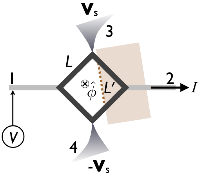
Figure 2: A diamond-shaped four-terminal loop. Voltage is applied to terminal 1, current is drawn out at 2 and Hall voltage and spin accumulation are measured at 3 and 4.

Consider a diamond-shaped loop, contacted by four leads, as sketched in Fig. 2. Low-bias spinless transport between the leads, in the presence of a magnetic flux threading the loop, is fully determined by two functions $g(\phi)$ and $t(\phi)$ (that depends on microscopic details), supposing for simplicity the structure is mirror symmetric with respect to the axis connecting leads 1 and 3 as well as leads 2 and 4. $t(\phi)$ [$g(\phi)$] is the flux-dependent conductance relating the current in lead 2 (3) induced by voltage in lead 1, while three other leads are grounded. By symmetry, the conductance for lead 4 equals $t(-\phi)$, which is in general different from $t(\phi)$. The coefficient $g(\phi)=g(-\phi)$, on the other hand, is symmetric in magnetic field. For the “transverse” conductance $t(\phi)$, we define symmetric and antisymmetric components:

$$t_{\pm}(\phi)=\frac{1}{2}\left[t(\phi)\pm t(-\phi)\right]\,.$$ (17)

Let us apply a small voltage bias $V$ to lead 1, grounding lead 2, and calculate the current $I$ in lead 2 and voltages $V_{3}$ and $V_{4}$ induced in leads 3 and 4, respectively, assuming leads 3 and 4 are disconnected from any external circuitry so that $I_{3}=I_{4}=0$. We find

$$V_{\pm}(\phi)=\frac{t_{\pm}(\phi)}{2t_{+}(\phi)}V\,,$$ (18)

where $V_{+}=(V_{4}+V_{3})/2$ and $V_{-}=(V_{4}-V_{3})/2$ is the Hall voltage. The induced current $I$ equals

$$I(\phi)=\left[g(\phi)+t_{+}(\phi)-\frac{t_{-}(\phi)^{2}}{t_{+}(\phi)}\right]V\,.$$ (19)

It therefore follows $I(\phi)=I(-\phi)$, as it should in effectively two-terminal conductor, according to time-reversal symmetry. The voltage difference $V_{-}(\phi)=-V_{-}(-\phi)$, on the other hand, is antisymmetric in magnetic field. This is an interference-induced Hall effect, in the absence of magnetic field within the wires.

Let us now return to the spin-orbit physics. Consider first a ring conductor with a uniform Rashba spin-orbit constant $\lambda$: $\hat{\mathbf{A}}=\lambda\mathbf{z}\times\hat{\boldsymbol{\sigma}}$. The effective magnetic flux is quadratic in $\lambda$ in this case, $\hat{\phi}_{f}\propto[\hat{A}_{x},\hat{A}_{y}]$:

$$\hat{\phi}_{f}\approx-\pi\left(\frac{L}{l_{\rm so}}\right)^{2}\phi_{0}\hat{\sigma}_{z}\,,$$ (20)

where $l_{\rm so}$ is the spin-orbit precession length (8). We are assuming here and henceforth weak spin-orbit coupling on the scale set by the ring size: $L\ll l_{\rm so}$. The flux governing the AC effect on the two-terminal conductance is therefore $\phi_{s}=-\pi(L/l_{\rm so})^{2}\phi_{0}$. At the same time, a spin Hall effect develops, which is quadratic in the SO strength:

$$V_{s4} =V_{4}(\phi_{s})-V_{4}(-\phi_{s})=2V_{-}(\phi_{s})$$

$$=\frac{t_{-}(\phi_{s})}{t_{+}(\phi_{s})}V\approx\frac{\phi_{s}\partial_{\phi}t|_{\phi\to 0}}{t}V\,,$$ (21)

where $V_{s4}=-V_{s3}$ are the $z$-axis spin accumulations induced in leads 3 and 4, respectively.

Next, suppose a top gate induces Rashba interaction only in a half-space. Let $L^{\prime}$ be the length of the gate edge overlapping the ring and $\mathbf{n}$ is the in-plane normal to the edge, pointing toward the region with a finite Rashba coupling $\lambda$, see Fig. 2. Using Eq. (5), we get

$$\hat{\phi}_{f}/\phi_{0}=\frac{L^{\prime}}{2l_{\rm so}}(\hat{\boldsymbol{\sigma}}\cdot\mathbf{n})\,.$$ (22)

Compare this result to Eq. (20). There are two important differences: Firstly, the spin-orbit inhomogeneity enhances the magnitude of the flux, making it linear in $\lambda$ rather than quadratic. Secondly, the spins are induced along the $\mathbf{n}$ direction determined by the edge orientation, rather than the 2DEG normal ($z$ axis) as in Eq. (20). Both AC and spin Hall effects discussed for the uniform $\lambda$ are similar in the present case, once we identify the new effective flux magnitude $\phi_{s}=(L^{\prime}/2l_{\rm so})\phi_{0}$ and the new spin quantization axis $\mathbf{n}$.

Finally, we note that the importance of the fictitious magnetic field (4) and the relation to the conventional Hall effect for the semiclassical boundary spin Hall physics was discussed in Ref. Tserkovnyak et al., , in a related but different context.

V Summary

In conclusion, we have shown that a spatially inhomogeneous SO interaction enhances the spin-interference effects in rings smaller than the spin-precession length. Transport can be understood in terms of the AB physics with fictitious spin-dependent magnetic fluxes. Spin injection in two-terminal rings and spin Hall effect in four-terminal rings are enhanced and controlled by the edge of the SO interaction inhomogeneity.