Anisotropic spin relaxation in quantum dots

Abstract

We study theoretically phonon-assisted spin relaxation of an electron confined in an elliptical quantum dot (QD) subjected to a tilted magnetic field. In the presence of both Rashba and Dresselhaus spin-orbit terms, the relaxation rate is anisotropic with respect to the in-plane field orientation. This anisotropy originates from the interference, at nonzero tilt angle, between the two spin-orbit terms. We show that, in a narrow range of magnetic field orientations, the relaxation rate exhibits anomalous sensitivity to variations of the QD parameters. In this range, the relative change in the relaxation rate with in-plane field orientation is determined solely by the spin-orbit coupling strengths and by the dot geometry. This allows simultaneous determination of both Rashba and Dresselhaus coupling parameters and the dot ellipticity from analysis of the angular dependence of the relaxation rate.

I introduction

Spin relaxation in semiconductor quantum dots (QDs) has recently attracted intense interest because of the possible use of the electron spin as a qubit.loss-pra98 Quantization of orbital states in a QD due to the zero-dimensional (0D) confinement leads to the suppression of traditional spin-relaxation mechanisms (e.g., D’yakonov-Perel) that are dominant in continuous systems. Indeed, recent experiments on GaAs QDs in a magnetic field $B$ have revealed extremely long spin-relaxation times (up to $T_{1}=170$ ms at $B\simeq 1.75$ T). tokura-nature02 ; hanson-prl03 ; elzerman-nature04 ; kroutvar-nature04 ; hanson-prl05 ; tokura-prl06 ; kastner-condmat06 For moderate and high fields ($B>1$ T), spin relaxation in QDs is dominated by phonon-assisted electronic transitions between Zeeman-split levels due to spin-orbit (SO) coupling. khaetskii-prb00 ; lyanda-prb02 ; golovach-prl04 ; bulaev-prb05 ; ulloa-prb05 ; falko-prl05 ; konemann-prl05 ; stano-prl06 There are two distinct types of SO couplings, one originating from bulk inversion asymmetry (Dresselhaus coupling) and the other from structural inversion asymmetry along the growth direction (Rashba coupling), that cause the admixture of orbital states with opposite spins. winkler-book In the case of circular QDs in a perpendicular magnetic field, the Rashba and Dresselhaus terms mix different pairs of levels, and can, in principle, be distinguished if one such pair provides the dominant relaxation channel. This is the case, for example, when adjacent orbital levels, coupled via the Rashba term, are brought into resonance with changing magnetic field.bulaev-prb05 However, in more realistic situations, deformations of the QD shape strongly alter the electronic spectrum austing-prb99 and, in general, the effects of the two SO contributions are not separable. valin-rodriguez-prb02

An important distinction between the Rashba and Dresselhaus terms is their different symmetry properties. The former, described by the Hamiltonian $\hat{H}_{R}=\alpha_{R}\bigl{(}\sigma_{x}\pi_{y}-\sigma_{y}\pi_{x}\bigr{)}$, possesses an in-plane rotational symmetry, while the latter, $\hat{H}_{D}=\alpha_{D}\bigl{(}\sigma_{x}\pi_{x}-\sigma_{y}\pi_{y}\bigr{)},$ does not.winkler-book Here ${\bm{\pi}}=-i{\bm{\nabla}}+e{\bf A}$, ${\bf A}$ being the vector potential, ${\bm{\sigma}}$ is the Pauli matrix vector, and $\alpha_{R}$ ($\alpha_{D}$) is Rashba (Dresselhaus) coupling constant (we set $\hbar=1$). This lack of rotational invariance for $\hat{H}_{D}$ leads to an in-plane momentum azimuthal anisotropy in the presence of both SO terms that was recently reported in transport experiments in quantum wells. marcus-prl03 ; ganichev-prl04 In a magnetic field, the anisotropy arises due to the interference between Rashba and Dresselhaus terms in the matrix elements falko-prb92 in the presence of an in-plane field component. In QDs, this anisotropy reveals itself as a modulation of the spin relaxation rate for different orientations of the in-plane field. golovach-prl04 ; falko-prl05 ; konemann-prl05 ; stano-prl06

Here we study the spin relaxation between Zeeman-split levels in elliptical QDs in a tilted magnetic field. We demonstrate that the interplay between SO interactions and QD geometry leads to dramatic changes in the relaxation rate in a certain range of field orientations for which Rashba and Dresselhaus contributions undergo destructive interference. Furthermore, in the vicinity of level anticrossings (see Fig. 1), the SO contribution to the relaxation rate factors out from the phonon one. This allows simultaneous determination of the parameters for both SO interactions and QD geometry from the azimuthal anisotropy of the differential (with respect to angle) relaxation rate.

The paper is organized as follows. In Section II we derive electronic spectrum of elliptical QD in a tilted magnetic field with both Rashba and Dresselhaus SO terms included. In Section III the spin relaxation rate between lowest levels is evaluated. Numerical results for GaAs dots are presented in Section IV.

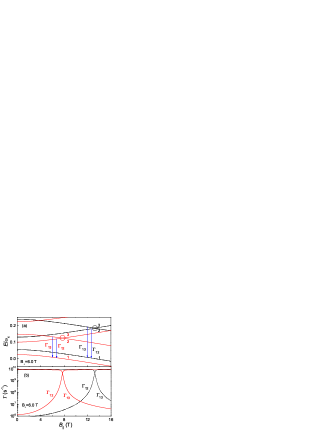
Figure 1: (Color online) (a) Energy levels and (b) relaxation rates $\Gamma_{12}$ and $\Gamma_{13}$ for circular (dashed line) and elliptical (solid line) QDs vs. in-plane field component $B_{||}$. Arrows in panel (a) indicate relevant transitions, and circles indicate resonance regions.

II Spin-Orbit coupling and electron states in elliptical QD in tilted magnetic field

We start with the electronic spectrum in an elliptical QD in the presence of SO interactions subjected to a tilted magnetic field

$${\bf B}={\bf B}_{\perp}+{\bf B}_{||}=B\bigl{(}\hat{x}\sin\theta\cos\varphi+\hat{y}\sin\theta\sin\varphi+\hat{z}\cos\theta\bigr{)},$$ (1)

where $\theta$ and $\varphi$ are the tilt and azimuthal angles, respectively. The system is described by the Hamiltonian $\hat{H}=\hat{H}_{0}+\hat{H}_{SO}+\hat{H}_{Z},$ where $\hat{H}_{0}={\bm{\pi}}^{2}/2m+V_{c}$ is the Hamiltonian of a 2D electron confined by the parabolic potential

$$V_{c}=m\bigl{(}\omega_{x}^{2}x^{2}+\omega_{y}^{2}y^{2}\bigr{)}/2,$$ (2)

$\omega_{x}$ and $\omega_{y}$ being the frequencies of the QD in-plane potential, $\hat{H}_{SO}=\hat{H}_{R}+\hat{H}_{D}$ is the SO term, and $\hat{H}_{Z}=\frac{1}{2}g^{\ast}\mu_{B}{\bm{\sigma}}\cdot{\bf B}$ is the Zeeman term ($m$, $g^{\ast}$ and $\mu_{B}$ stand for the electron effective mass, $g$ factor and Bohr magneton). For sufficiently strong 2D confinement, the orbital effect of the in-plane field can be neglected and $\hat{H}_{0}$ depends only on the perpendicular field component via ${\bf A}=\frac{B_{\perp}}{2}\bigl{(}-y,x,0\bigr{)}$ (in symmetrical gauge). Using the transformation

$$\pi_{x}=a_{1}P_{1}-a_{2}P_{2},~{}\pi_{y}=-m\omega_{1}b_{1}Q_{1}+m\omega_{2}b_{2}Q_{2}$$

$$x=a_{1}Q_{1}-a_{2}Q_{2},~{}y=\frac{b_{1}}{m\omega_{1}}P_{1}-\frac{b_{2}}{m\omega_{2}}P_{2},\qquad$$ (3)

$P_{j}$ and $Q_{j}$ ($j=1,2$) being canonical momenta and coordinates, the Hamiltonian $\hat{H}_{0}$ can be brought to the canonical form of two uncoupled oscillators with frequencies galkin-prb04

$$\omega_{1,2}=\frac{1}{2}\biggl{[}\sqrt{\bigl{(}\omega_{x}+\omega_{y}\bigr{)}^{2}+\omega_{c}^{2}}\pm\sqrt{\bigl{(}\omega_{x}-\omega_{y}\bigr{)}^{2}+\omega_{c}^{2}}\biggr{]},$$ (4)

where $\omega_{c}=eB_{\perp}\bigl{/}m$ is the cyclotron frequency and the coefficients $a_{j}$ and $b_{j}$ are given by

$$a_{j}=\omega_{c}\omega_{j}/D_{j},~{}b_{j}=\bigl{(}\omega_{x}^{2}-\omega^{2}_{j}\bigr{)}/D_{j}$$ (5)

with $D_{j}=\bigl{[}\bigl{(}\omega_{x}^{2}-\omega_{j}^{2}\bigr{)}^{2}+\omega_{x}^{2}\omega_{c}^{2}\bigr{]}^{1/2}$. In the absence of SO coupling, the spectrum represents two ladders of equidistant levels (for each spin projection) with energies

$$E^{(0)}_{n_{1}n_{2}\pm}=\bigl{(}n_{1}+1\bigl{/}2\bigr{)}\omega_{1}+\bigl{(}n_{2}+1\bigl{/}2\bigr{)}\omega_{2}\pm\omega_{Z},$$ (6)

where $\omega_{Z}=\frac{1}{2}g^{\ast}\mu_{B}B$ is the Zeeman energy.

The SO term $\hat{H}_{SO}=\hat{H}_{D}+\hat{H}_{R}$ causes an admixture of the oscillator states $|n_{1}n_{2}\rangle_{\pm}$ with different orbital ($n_{j}$) and spin ($\pm$) quantum numbers. In a titled field, the calculation of the SO matrix elements is carried out in two steps (see Appendix A). First, the spin operators $\bm{\sigma}$ in $\hat{H}_{SO}$ are rotated in spin space to align the spin-quantization axis along the total field B. Second, the orbital operators $\bm{\pi}$ in $\hat{H}_{SO}$ are expressed via new canonical variables $P_{j}$, $Q_{j}$. The expressions for the general matrix elements are provided in Appendix A; for the lowest adjacent levels with opposite spins corresponding to the $\omega_{2}$ ladder, they have the form

$${}_{\pm}\langle 01\bigl{|}\hat{H}_{SO}\bigr{|}00\rangle_{\mp}\qquad\qquad\qquad\qquad\qquad\qquad\qquad\qquad$$

$$=\frac{\alpha_{R}}{l_{2}\sqrt{2}}\Bigl{[}\bigl{(}b_{2}\cos\theta\pm a_{2}\bigr{)}\cos\varphi+i\bigl{(}a_{2}\cos\theta\pm b_{2}\bigr{)}\sin\varphi\Bigr{]}$$

$$-\frac{i\alpha_{D}}{l_{2}\sqrt{2}}\Bigl{[}\bigl{(}a_{2}\cos\theta\mp b_{2}\bigr{)}\cos\varphi-i\bigl{(}b_{2}\cos\theta\mp a_{2}\bigr{)}\sin\varphi\Bigr{]},$$ (7)

where $l_{j}=(m\omega_{j})^{-1/2}$. These matrix elements explicitly depend on the tilt, $\theta$, and azimuthal, $\varphi$, angles as well as on the QD geometry encoded in the coefficients $a_{j},b_{j}$. In general, the magnitude of SO coupling is small compared to the level separation, $\alpha\bigl{/}l_{j}\ll\omega_{j}$, and, accordingly, the SO-induced level admixture is weak. However, the level mixing gets strongly enhanced near the resonance, i.e., when the spacing between adjacent levels is of the order of the SO energy: $\omega_{2}-\omega_{Z}\sim\alpha_{R,D}/l_{2}$ (see Fig. 1). This can be achieved, e.g., by varying the Zeeman energy with the tilt angle $\theta$. The corresponding anticrossing gap,

$$\Delta=2\bigl{|}{}_{+}\langle 01\bigr{|}\hat{H}_{SO}\bigl{|}00\rangle_{-}\bigr{|},$$ (8)

is evaluated from Eq. (II) as

$$\mbox{}\Delta^{2}\!=\!\frac{\alpha_{R}^{2}}{l_{2}^{2}}\Bigl{[}\bigl{(}b_{2}\cos\theta+a_{2}\bigr{)}^{2}\!\cos^{2}\varphi+\bigl{(}b_{2}+a_{2}\cos\theta\bigr{)}^{2}\!\sin^{2}\varphi\Bigr{]}$$

$$\,\,+\frac{\alpha_{D}^{2}}{l_{2}^{2}}\Bigl{[}\bigl{(}b_{2}\cos\theta-a_{2}\bigr{)}^{2}\!\sin^{2}\varphi+\bigl{(}b_{2}-a_{2}\cos\theta\bigr{)}^{2}\!\cos^{2}\varphi\Bigr{]}$$

$$\,\,+\frac{\alpha_{R}\alpha_{D}}{l_{2}^{2}}\bigl{(}a_{2}^{2}+b_{2}^{2}\bigr{)}\sin^{2}\theta\sin 2\varphi.$$ (9)

The gap magnitude is governed by the angle-dependent interference between Rashba and Dresselhaus terms. Importantly, in elliptical QDs, such interference depends on the dot geometry via the coefficients $a_{j}$, $b_{j}$.

Thus, near the resonance, $\omega_{2}-\omega_{Z}\sim\Delta$, the energies of the lowest excited states,

$$E_{2,3}=\omega_{2}\mp\frac{1}{2}\sqrt{(\omega_{2}-\omega_{Z})^{2}+\Delta^{2}},$$ (10)

acquire a strong angular dependence. At the same time, the phonon-assisted transitions between these states $|j\rangle$ ($j=2,3$) and the ground state $|1\rangle$ are enhanced due to the strong admixture of constituent orbital levels (see Fig. 1). As a result, the spin relaxation becomes anisotropic with respect to the in-plane field orientation $\varphi$. As we show below, the relaxation exhibits anomalous sensitivity of to the system parameters in a narrow range of $\varphi$ where the SO terms interfere destructively.

III Phonon-assisted spin relaxation

The transition rate between state $|j\rangle$ and the ground state $|1\rangle$ is given by

$$\Gamma_{1j}=2\pi\sum_{{\bf Q}\lambda}|\langle 1|U_{\lambda}|j\rangle|^{2}\delta\bigl{(}E_{1}-E_{j}+\omega_{{\bf Q}\lambda}\bigr{)},$$ (11)

where the sum runs over acoustic phonon modes $\lambda$ with dispersion $\omega_{{\bf Q}\lambda}=c_{\lambda}Q$, $c_{\lambda}$ being the sound velocity, and 3D momenta ${\bf Q}=({\bf q},q_{z})$. The transition matrix element is a product of phonon and electron contributions,

$$\langle 1|U_{\lambda}|j\rangle=M_{\lambda}({\bf Q})\langle 1|e^{i{\bf Q}{\bf R}}|j\rangle,$$ (12)

where the phonon part,

$$M_{\lambda}({\bf Q})=\Lambda_{\lambda}({\bf Q})+i\Xi_{\lambda}({\bf Q}),$$ (13)

includes piezoelectric, $\Lambda_{\lambda}$, and deformation, $\Xi_{\lambda}$, contributions.gantmakher-book In the numerical calculations below, we include both longitudinal and two transverse piezoelectric acoustical modes. The details can be found in Appendix B. The electron matrix element can, in turn, be decomposed into a product of transverse and in-plane contributions,

$$\langle 1|e^{i{\bf Q}{\bf R}}|j\rangle=f_{z}(q_{z})f_{1j}(\bf q).$$ (14)

The transverse contribution $f_{z}(q_{z})$ is determined by the 2D confinement, assumed parabolic below, while the in-plane contribution $f_{1j}(\bf q)$ is evaluated as follows.

Not too far from the resonance region, $\bigl{|}\frac{\omega_{2}-\omega_{Z}}{\omega_{2}+\omega_{Z}}\bigr{|}\ll 1$, it is sufficient to restrict calculations to the lowest four levels of the $\omega_{2}$ ladder. The states $|2\rangle$ and $|3\rangle$, corresponding to the anticrossing levels, are superpositions of unperturbed states,

$$|j\rangle=d^{(j)}_{00-}|00\rangle_{-}+d^{(j)}_{01+}|01\rangle_{+},$$ (15)

while the ground state acquires a small admixture from the upper orbital of opposite spin,

$$\bigl{|}1\bigr{\rangle}=d^{(1)}_{00+}\bigl{|}00\rangle_{+}+d^{(1)}_{01-}\bigl{|}01\rangle_{-}.$$ (16)

The coefficients $d$ are obtained as

$$d^{(3)}_{01+}=d^{(2)}_{00-}=\bigl{(}1+e^{-2\beta}\bigr{)}^{-1/2},$$

$$d^{(3)}_{00-}=-d^{(2)\ast}_{01+}=e^{i\eta}\bigl{(}1+e^{2\beta}\bigr{)}^{-1/2},$$

$$d^{(1)}_{00+}=\bigl{(}1+\xi^{2}\bigr{)}^{-1/2},\,\,d^{(1)}_{01-}=\xi^{\ast}\bigl{(}1+\xi^{2}\bigr{)}^{-1/2},$$ (17)

where

$$\xi=\frac{{}_{-}\bigl{\langle}01\bigl{|}\hat{H}_{SO}\bigr{|}00\bigr{\rangle}_{+}}{\omega_{2}+\omega_{Z}}\sim\frac{\alpha_{R,D}}{l_{2}(\omega_{2}+\omega_{Z})}$$ (18)

is the ratio of SO and orbital energies, while $\eta=\arg\bigl{(}{}_{+}\langle 01\bigl{|}\hat{H}_{SO}\bigr{|}00\rangle_{-}\bigr{)}$ is the phase of the SO matrix element. The parameter $\beta$ characterizes the proximity to the resonance:

$$\sinh\beta=(\omega_{2}-\omega_{Z})/\Delta$$ (19)

is the detuning in units of the anticrossing gap. In deriving Eqs. (III), we neglected higher-order terms in the SO coupling suppressed by the additional factor $\bigl{|}\xi\bigr{|}\ll 1$. In the resonance region $\beta\sim 1$, the coefficients $d^{(2)}\sim d^{(3)}\sim 1$, i.e., the levels 2 and 3 are well hybridized. Away from the resonance, $\Delta\ll|\omega_{2}-\omega_{Z}|\ll(\omega_{2}+\omega_{Z})$, corresponding to $|\beta|\gg 1$, the eigenstates 2 and 3 are mainly determined by the unperturbed states $|00\rangle_{-}$ and $|01\rangle_{+}$ (and vice versa) to the left (right) from the resonance region.

In terms of the coefficients $d$, the 2D matrix element takes the form

$$f_{1j}({\bf q})=d^{(1)}_{01-}d^{(j)\ast}_{00-}f_{0001}({\bf q})+d^{(1)}_{00+}d^{(j)\ast}_{01+}f_{0100}({\bf q}),$$ (20)

with $f_{m^{\prime}n^{\prime}mn}=\langle m^{\prime}n^{\prime}|e^{i{\bf qr}}|mn\rangle.$ The relevant elements are (see Appendix C)

$$f_{0001}=f_{0100}^{\ast}=\frac{il_{2}q}{\sqrt{2}}e^{-(a_{1}^{2}l_{1}^{2}+a_{2}^{2}l_{2}^{2})q^{2}/4}(-a_{2}\cos\phi+ib_{2}\sin\phi),$$ (21)

with $\phi=\arg(\bf q)$. We then obtain

$$f_{1j}=-\frac{il_{2}q}{\sqrt{2}}e^{-(a_{1}^{2}l_{1}^{2}+a_{2}^{2}l_{2}^{2})q^{2}/4}\bigl{[}F^{(j)}_{1}e^{-i\phi}+F^{(j)}_{2}e^{i\phi}\bigr{]},$$ (22)

where

$$F^{(j)}_{1}=\frac{1}{2}\Bigl{[}(a_{2}+b_{2})d^{(j)}_{01+}d^{(1)\ast}_{00+}+(a_{2}-b_{2})d^{(j)}_{00-}d^{(1)^{\ast}}_{01-}\Bigr{]},\,\,$$

$$F^{(j)}_{2}=\frac{1}{2}\Bigl{[}(a_{2}-b_{2})d^{(j)}_{01+}d^{(1)^{\ast}}_{00+}+(a_{2}+b_{2})d^{(j)}_{00-}d^{(1)^{\ast}}_{01-}\Bigr{]}.\,\,$$ (23)

Substituting Eq. (22) into the full transition matrix element,

$$\langle 1|U_{\lambda}|j\rangle=M_{\lambda}({\bf Q})f_{z}(q_{z})f_{1j}(\bf q),$$ (24)

the scattering rate $\Gamma_{1j}$ is obtained by summing up over phonon modes in a standard manner khaetskii-prb00 ; lyanda-prb02 ; golovach-prl04 ; bulaev-prb05 ; ulloa-prb05 (see Appendix B). The result is the product

$$\Gamma_{1j}=G_{1j}\bigl{(}\varphi\bigr{)}W_{j},\ \ \ j=2,3$$ (25)

where the geometric factor

$$G_{1j}=\bigl{|}F^{\left(j\right)}_{1}\bigr{|}^{2}+\bigl{|}F^{\left(j\right)}_{2}\bigr{|}^{2}$$ (26)

is determined only by the SO-induced admixture of electronic states, encoded in the coefficients $d$, while the phonon factor $W_{j}$ describes the probability of phonon-assisted transitions between levels separated by energy $E_{j}-E_{1}$ (see Appendix B). Note that $W_{j}$ are nearly independent of the SO coupling; in the resonance region, the SO contribution to $W_{j}$ is $\sim\xi^{2}\ll 1$ and can be neglected.

Thus, near the resonance, the dependence of scattering rate $\Gamma$ on the SO parameters and, accordingly, on the azimuthal angle $\varphi$, comes only through the geometric factor $G_{1j}$. Remarkably, this factor can be extracted directly from the experimental data via the differential relaxation rate normalized to its value at some angle (e.g., $\varphi=0$):

$$\frac{\Delta\Gamma_{j}}{\Gamma}=\frac{\Gamma_{1j}\bigl{(}\varphi\bigr{)}-\Gamma_{1j}\bigl{(}0\bigr{)}}{\Gamma_{1j}\bigl{(}0\bigr{)}}=\frac{G_{1j}\bigl{(}\varphi\bigr{)}-G_{1j}\bigl{(}0\bigr{)}}{G_{1j}\bigl{(}0\bigr{)}},$$ (27)

where the r.h.s. is independent of the phonon contribution.

IV Discussion and numerical results

Below we present our numerical results for spin relaxation rates in a GaAs QD. Calculations were performed for a parabolic confining potential with $\omega_{x}=2$ meV and $\omega_{y}=1.33$ meV, corresponding to the ellipticity $\omega_{x}\bigl{/}\omega_{y}=3\bigr{/}2$. For comparison, results for the circular QD ($\omega_{x}=\omega_{y}=2$ meV) are presented too. We choose the parabolic transverse confinement with $l_{z}=4$ nm. The values of the SO constants, if not specified otherwise, in GaAs were taken as $\alpha_{R}=5$ meVÅ and $\alpha_{D}=16.25$ meVÅ, while the phonon parameters were taken from Ref. gantmakher-book, (see Appendix B).

In Fig. 1 we plot the lowest energy levels and relaxation rates for both circular and elliptical QDs as a function of the in-plane field $B_{||}$ at fixed $B_{\perp}=6.0$ T and $\varphi=0$. For chosen parameters, the level anticrossings at $\omega_{2}=\omega_{Z}$, indicated by circled regions, for elliptical QDs are achieved at lower $B_{||}$ due to a weaker confinement along the $y$ axis [see Fig. 1(a)]. The relaxation rates $\Gamma_{12}$ and $\Gamma_{13}$ are plotted in Fig. 1(b). The sharp increase in $\Gamma_{12}$ ($\Gamma_{13}$) is caused by a stronger SO-induced admixture of the $\bigl{|}00\bigr{\rangle}_{-}$ and $\bigl{|}01\bigr{\rangle}_{+}$ states as one approaches to the resonance from the left (right). To the right of the resonance ($\omega_{Z}>\omega_{2}$), $\Gamma_{12}$ is dominated by the orbital transition between states $\bigl{|}00\bigr{\rangle}_{+}$ and $\bigl{|}01\bigr{\rangle}_{+}$; so is $\Gamma_{13}$ to the left of the resonance ($\omega_{Z}<\omega_{2}$). The flat $B_{||}$ dependence in these regions is because in a narrow 2D layer the orbital wave functions depend only on $B_{\perp}$. Apart from the magnitude of $\Gamma$, the overall behavior is similar for circular and elliptical QDs.

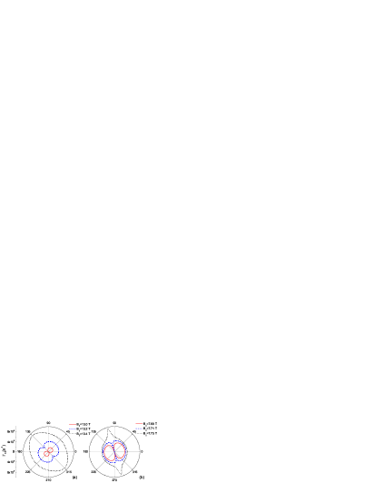
Figure 2: (Color online) Angular dependence of the relaxation rate $\Gamma_{12}$ for (a) circular and (b) elliptical QDs for $B_{\perp}=6.0$ T and several values of $B_{||}$.

In Fig. 2, we plot the relaxation rate $\Gamma_{12}$ as a function of in-plane field orientation $\varphi$ at several values of its magnitude $B_{||}$ in the resonance region. A strong azimuthal anisotropy is apparent: at certain angles, $\Gamma_{12}$ reaches minima that turn into maxima as $B_{||}$ sweeps through the resonance. For a circular QD, the extrema of $\Gamma_{12}$ occur at $\varphi=\pm\pi\bigl{/}4$ regardless of the values of $\alpha_{R}$ and $\alpha_{D}$ [see Fig. 2(a)]. This anisotropy originates from the angular dependence of the anticrossing gap $\Delta\bigl{(}\varphi\bigr{)}$. Indeed, in the resonance region, $|\omega_{2}-\omega_{Z}|\bigl{/}\Delta\sim 1$, the SO contribution to $\Gamma_{12}$ takes the simple form

$$G_{12}\bigl{(}\varphi\bigr{)}=\bigl{(}a_{2}^{2}+b_{2}^{2}\bigr{)}\Biggl{(}1-\frac{\omega_{2}-\omega_{Z}}{\bigl{[}\Delta^{2}+\bigl{(}\omega_{2}-\omega_{Z}\bigr{)}^{2}\bigr{]}^{1/2}}\Biggr{)}.$$ (28)

For a circular QD, the expression (II) for the gap simplifies to falko-prb92 ; golovach-prl04

$$\Delta^{2}=\frac{\omega_{2}}{\Omega}\bigl{(}\lambda_{D}^{2}+\lambda_{R}^{2}+2\lambda_{D}\lambda_{R}\sin 2\varphi\bigr{)}$$ (29)

with $\lambda_{D}=\alpha_{D}\sin^{2}(\theta/2)/l_{2}$ and $\lambda_{R}=\alpha_{R}\sin^{2}(\theta/2)/l_{2},$ so the extrema of $\Delta$ at $\varphi=\pm\pi/4$ translate into the extrema of $G$. In contrast, in elliptical QDs, the angular dependence of $\Gamma$ depends on the system parameters [see Fig. 2(b)]. The additional asymmetry introduced by the QD ellipticity modifies the interference between Rashba and Dresselhaus terms and shifts the extrema away from $\pm\pi/4$. The extrema of $\Delta$, Eq. (II), now depend on both the QD ellipticity and the SO parameters, and occur at

$$\tan 2\varphi_{e}=-2\frac{\alpha_{R}\alpha_{D}}{\alpha_{R}^{2}-\alpha_{D}^{2}}\frac{a_{2}^{2}+b_{2}^{2}}{a_{2}^{2}-b_{2}^{2}}.$$ (30)

For the parameters of Fig. 2(b), $\varphi_{e}=106^{\rm o}$.

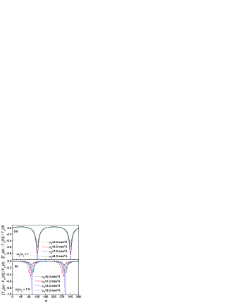
Figure 3: (Color online) Angular dependence of the differential relaxation rates for (a) circular and (b) elliptical QDs for several values of the coefficients $\alpha_{R}$ at $B_{\perp}=6.0$ T and $B_{||}=13.2$ T (a) and $B_{||}=7.7$ T (b).

Such interplay between QD geometry and SO interactions suggests a way to simultaneously determine both SO couplings and QD ellipticity from the measured angular dependence of the differential relaxation rate $\Delta\Gamma/\Gamma$, Eq. (27). In the resonance region, the phonon contribution $W_{j}$ drops out, as does the prefactor in Eq. (28), so $\Delta\Gamma/\Gamma$ is determined solely by the anticrossing gap $\Delta(\varphi,\omega_{x},\omega_{y})$. The angular dependence of $\Delta\Gamma\bigl{/}\Gamma$ is shown in Fig. 3 for several values of Rashba coupling $\alpha_{R}$ which can be varied, e.g., with an external electric field.winkler-book For a circular QD, change in $\alpha_{R}$ does not affect the minima positions at $\varphi=-\pi\bigl{/}4$, as discussed above; however, the modulation depth varies strongly [see Fig. 3(a)]. Note that the $\alpha_{R}$ dependence is nonmonotonic; the deepest minimum occurs for the almost complete destructive interference of the SO terms at $\alpha_{R}\bigl{/}\alpha_{D}\approx\tan^{2}(\theta/2)$.

Deviations from circular QD shape give rise to angular dispersion of spin relaxation in the parameter space. For elliptical QDs, variations of $\alpha_{R}$ shift the minima positions of $\Delta\Gamma\bigl{/}\Gamma$ [see Fig. 3(b)]. In fact, the sensitivity of $\Delta\Gamma\bigl{/}\Gamma$ to the system parameters is drastically enhanced for $\varphi$ in the vicinity of the critical angles $\varphi_{e}$, Eq. (30), for which the destructive interference between the Rashba and Dresselhaus terms is strongest. Thus, a scan of the angular dependence of the experimental differential relaxation rate in this narrow domain would enable an unambiguous extraction of both SO and QD geometry parameters.

V conclusion

In summary, we proposed a method for simultaneous extraction of both the spin-orbit constants as well as the quantum dot shape from the angular anisotropy of the differential spin relaxation rate in a tilted field. The underlying mechanism is based upon the enhanced sensitivity of phonon-assisted spin-flip transitions to the system parameters in the vicinity of level anticrossings. This sensitivity arises from destructive interference between the SO terms in a narrow domain of in-plane field orientations in the presence of asymmetric confinement. Note that such interplay between SO interactions and QD geometry cannot be captured by simplified descriptions of elliptical QDs using circular QDs with effective parameters.tokura-nature02

VI acknowledgement

This work was supported by the NSF under Grant No. DMR-0606509 and by the DoD under contract No. W912HZ-06-C-0057.

Appendix A Spin-orbit matrix elements in tilted field

Here we describe calculation of the SO matrix elements in elliptical QD in tilted magnetic field. It is convenient to work in the basis in which Zeeman term is diagonal. Therefore, we choose the spin quantization axis along the total field and perform the corresponding rotation of the Pauli matrices:

$$\sigma_{x} \rightarrow \sigma_{x}\cos\theta\cos\varphi-\sigma_{y}\sin\varphi+\sigma_{z}\sin\theta\cos\varphi,$$

$$\sigma_{y} \rightarrow \sigma_{x}\cos\theta\sin\varphi+\sigma_{y}\cos\varphi+\sigma_{z}\sin\theta\sin\varphi,$$

$$\sigma_{z} \rightarrow -\sigma_{x}\sin\theta+\sigma_{z}\cos\theta.$$ (31)

The orbital variables are chosen to diagonalize the free Hamiltonian $\hat{H}_{0}$ with the help of transformation Eq. (II). In this basis, the Hamiltonian $\hat{H}_{0}+\hat{H}_{Z}$ is diagonal in both orbital and spin spaces, with the eigenstates $|n_{1},n_{2}\rangle_{\pm}$ corresponding to two uncoupled oscillators with energies given by Eq. (6). The calculation of matrix elements of $\hat{H}_{SO}$ between these eigenstates is convenient to perform by utilizing rising $\hat{c}_{j}^{\dagger}=\frac{1}{\sqrt{2}}\Bigl{(}\frac{Q_{j}}{l_{j}}-il_{j}P_{j}\Bigr{)}$ and lowering $\hat{c}_{j}=\frac{1}{\sqrt{2}}\Bigl{(}\frac{Q_{j}}{l_{j}}+il_{j}P_{j}\Bigr{)}$ operators. The corresponding non-zero matrix elements have the form

$${}_{\pm}\langle n_{1},n_{2}\bigl{|}\hat{H}_{SO}\bigr{|}n_{1},n_{2}-1\rangle_{\mp}=\sqrt{\frac{n_{2}}{2}}\biggl{(}\frac{\alpha_{R}}{l_{2}}\Bigl{[}\bigl{(}b_{2}\cos\theta\pm a_{2}\bigr{)}\cos\varphi+i\bigl{(}a_{2}\cos\theta\pm b_{2}\bigr{)}\sin\varphi\Bigr{]}$$

$$+i\frac{\alpha_{D}}{l_{2}}\Bigl{[}\bigl{(}-a_{2}\cos\theta\pm b_{2}\bigr{)}\cos\varphi+i\bigl{(}b_{2}\cos\theta\mp a_{2}\bigr{)}\sin\varphi\Bigr{]}\biggr{)},$$

$${}_{\pm}\langle n_{1},n_{2}\bigl{|}\hat{H}_{SO}\bigr{|}n_{1},n_{2}-1\rangle_{\pm}=\pm\sqrt{\frac{n_{2}}{2}}\biggl{[}\frac{\alpha_{R}}{l_{2}}\bigl{(}b_{2}\cos\varphi+ia_{2}\sin\varphi\bigr{)}-i\frac{\alpha_{D}}{l_{2}}\bigl{(}a_{2}\cos\varphi-ib_{2}\sin\varphi\bigr{)}\biggr{]}\sin\theta$$

$${}_{\pm}\langle n_{1},n_{2}\bigl{|}\hat{H}_{SO}\bigr{|}n_{1}-1,n_{2}\rangle_{\mp}=\sqrt{\frac{n_{1}}{2}}\biggl{(}\frac{\alpha_{R}}{l_{1}}\Bigl{[}\bigl{(}-b_{1}\cos\theta\mp a_{1}\bigr{)}\cos\varphi\pm i\bigl{(}b_{1}\pm a_{1}\cos\theta\bigr{)}\sin\varphi\Bigr{]}$$

$$+i\frac{\alpha_{D}}{l_{1}}\Bigl{[}\bigl{(}a_{1}\cos\theta\mp b_{1}\bigr{)}\cos\varphi+i\bigl{(}-b_{1}\cos\theta\pm a_{1}\bigr{)}\sin\varphi\Bigr{]}\biggr{)},$$

$${}_{\pm}\langle n_{1},n_{2}\bigl{|}\hat{H}_{SO}\bigr{|}n_{1}-1,n_{2}\rangle_{\pm}=\mp\sqrt{\frac{n_{1}}{2}}\biggl{[}\frac{\alpha_{R}}{l_{1}}\bigl{(}b_{1}\cos\varphi+ia_{1}\sin\varphi\bigr{)}-i\frac{\alpha_{D}}{l_{1}}\bigl{(}a_{1}\cos\varphi-ib_{1}\sin\varphi\bigr{)}\biggr{]}\sin\theta.$$ (32)

Note that $\hat{H}_{SO}$ does not couple states of different oscillators. The second and fourth relations in Eqs. (A) describe SO-induced transitions without spin-flip that are absent in perpendicular field ($\theta=0$). Here, both Rashba and Dresselhaus terms contribute to the coupling between same levels. In contrast, for circular QD in perpendicular field with $\omega_{x}=\omega_{y}=\omega_{0}$, the two SO terms only couple different levels:

$${}_{+}\langle n_{1},n_{2}\bigl{|}\hat{H}_{SO}\bigr{|}n_{1},n_{2}-1\rangle_{-}=\frac{\alpha_{R}}{l_{2}}\sqrt{\frac{n_{2}\omega_{2}}{\Omega}}\,$$

$${}_{-}\langle n_{1},n_{2}\bigl{|}\hat{H}_{SO}\bigr{|}n_{1},n_{2}-1\rangle_{+}=-i\frac{\alpha_{D}}{l_{2}}\sqrt{\frac{n_{2}\omega_{2}}{\Omega}},$$ (33)

where $\Omega=\sqrt{\omega_{0}^{2}+\omega_{c}^{2}/4}$ and $\omega_{1,2}=\Omega\pm\omega_{c}/2$ (analogous relations hold for the $\omega_{1}$ ladder).

Appendix B Electron-phonon matrix elements

B.1 Phonon matrix element $M(\bf Q)$

The phonon-assisted transition rate is given by

$$\Gamma_{1j}=2\pi\sum_{{\bf Q}\lambda}|\langle 1|U_{\lambda}|j\rangle|^{2}\delta\bigl{(}E_{1}-E_{j}+c_{\lambda}Q\bigr{)}$$ (34)

where the operator of electron-phonon interaction $U_{\lambda}$ has the form gantmakher-book

$$U_{\lambda}=\bigl{(}2\rho Qc_{\lambda}V\bigr{)}^{-1/2}\bigl{(}eA_{{\bf Q}\lambda}+iQD_{{\bf Q}\lambda}\bigr{)}e^{i{\bf Q}{\bf R}}\bigl{(}b_{{\bf Q}\lambda}+b^{\dagger}_{-{\bf Q}\lambda}\bigr{)}.$$ (35)

Here,

$$A_{{\bf Q}\lambda}=\frac{h_{14}}{Q^{2}\kappa}\bigl{(}q_{x}q_{y}e^{\lambda}_{z}+q_{x}q_{z}e^{\lambda}_{y}+q_{y}q_{z}e^{\lambda}_{x}\bigr{)}$$ (36)

is the amplitude of electric field created by phonon strain, and deformation potential $D_{{\bf Q}\lambda}$ contains only longitudinal acoustical (LA) component, $D_{{\bf Q}\lambda}=\delta_{\lambda,LA}\Xi_{0}$, with $\Xi_{0}$ being a constant of the deformation potential. Also, $b^{\dagger}_{{\bf Q}\lambda}$ ($b_{{\bf Q}\lambda}$) creates (annihilates) phonon with dispersion $\omega_{{\bf Q}\lambda}=Qc_{\lambda}$, $V$ is the QD volume, ${\bf R}=({\bf r},z)$ is 3D electron radius vector, $\rho$ is the crystal mass density, ${\bf e}^{\lambda}$ is the phonon polarization vector, $c_{\lambda}$ is sound velocity, $h_{14}$ is bulk phonon constant, $\kappa$ is the static dielectric constant. Accordingly, the phonon part $M_{\lambda}({\bf Q})$ of the transition matrix element $\langle 1|U_{\lambda}|j\rangle$ includes both piezoelectric $\Lambda_{\lambda}$ and deformation $\Xi_{\lambda}$ contributions:

$$M_{\lambda}({\bf Q})=\Lambda_{\lambda}({\bf Q})+i\Xi_{\lambda}({\bf Q})$$ (37)

with piezoelectric part containing LA and two transverse acoustical (TA1, TA2) modes. Since polarization directions are given as

$${\bf e}^{L}=\hat{x}\sin\theta_{\bf Q}\cos\phi+\hat{y}\sin\theta_{\bf Q}\sin\phi+\hat{z}\cos\theta_{\bf Q},$$

$${\bf e}^{TA1}=\hat{x}\cos\theta_{\bf Q}\cos\phi+\hat{y}\cos\theta_{\bf Q}\sin\phi-\hat{z}\sin\theta_{\bf Q},$$

$${\bf e}^{TA2}=-\hat{x}\sin\phi+\hat{y}\cos\phi$$ (38)

[$\theta_{\bf Q}=\arcsin\bigl{(}q\bigl{/}Q\bigr{)}$, $\phi=\arg(\bf q)$], one gets

$$\Xi_{LA}\bigl{(}{\bf Q}\bigr{)}=\Xi_{0}A_{LA}\sqrt{Q},$$ (39)

where, as mentioned above, only $LA$ mode is present for $\Xi_{\lambda}$. For $\Lambda_{\lambda}$ one obtains

$$\Lambda_{LA}\bigl{(}{\bf Q}\bigr{)}=\frac{3}{2}\Lambda_{0}A_{LA}\frac{q^{2}q_{z}}{Q^{7/2}}\sin 2\phi,$$

$$\Lambda_{TA1}\bigl{(}{\bf Q}\bigr{)}=\frac{1}{2}\Lambda_{0}A_{TA}\biggl{(}2\frac{q_{z}^{2}}{q^{2}}-1\biggr{)}\frac{q^{3}}{Q^{7/2}}\sin 2\phi,$$

$$\Lambda_{TA2}\bigl{(}{\bf Q}\bigr{)}=\Lambda_{0}A_{TA}\frac{qq_{z}}{Q^{5/2}}\cos 2\phi.$$ (40)

In the above equations, $\Lambda_{0}=eh_{14}/\kappa$, and $A_{\lambda}=\bigl{(}2\rho Vc_{\lambda}\bigr{)}^{-1/2}$. The sound velocities of the transverse and longitudinal modes are $c_{TA1}=c_{TA2}\equiv c_{TA}$ and $c_{LA}$, respectively. For GaAs, the parameter values are $eh_{14}=0.14$ eV/Å, $\Xi_{0}=7$ eV, $c_{LA}=5.14\times 10^{3}$ m/s, $c_{TA}=3.03\times 10^{3}$ m/s, $\rho=5.31$ g/${\rm cm}^{3}$, and $\kappa=12.79$.

B.2 Expressions for $W_{j}$

To obtain Eq. (25), one has to perform integration over phonon modes in Eq. (34). The transition matrix element has the form $\langle 1|U_{\lambda}|j\rangle=M_{\lambda}({\bf Q})f_{z}(q_{z})f_{1j}(\bf q)$, where $M_{\lambda}({\bf Q})$ is described in the previous subsection, $f_{z}(q_{z})$ is provided in the next section, and $f_{1j}$ is given by Eq. (22). Then, integration over $q_{z}$ eliminates $\delta$-functions in Eq. (34). Subsequent $\phi$-integration eliminates terms linear in $F^{\left(j\right)}_{i}$. Remaining $q$-integration leads to Eq. (25) where the phonon factor $W_{j}$ is given by

$$W_{j}=\frac{1}{2\pi}\sum_{\lambda}\int_{0}^{\frac{\Delta E_{j}}{c_{\lambda}}}\frac{A_{\lambda}\bigl{(}q\bigr{)}q^{3}dq}{\sqrt{\Bigl{(}\frac{\Delta E_{j}}{c_{\lambda}}\Bigr{)}^{2}-q^{2}}}\qquad\qquad\qquad$$

$$\times e^{-\bigl{(}a_{1}^{2}l_{1}^{2}+a_{2}^{2}l_{2}^{2}\bigr{)}q^{2}/2}\Biggl{|}f_{z}\Biggl{(}\sqrt{\biggl{(}\frac{\Delta E_{j}}{c_{\lambda}}\biggr{)}^{2}-q^{2}}\Biggr{)}\Biggr{|}^{2},$$ (41)

with summation running over all phonon modes: deformation ($Def$), longitudinal and transverse acoustical:

$$A_{Def}\bigl{(}q\bigr{)}=\Xi_{0}^{2}A_{LA}^{2}\frac{2\bigl{(}\Delta E_{j}\bigr{)}^{2}}{c_{LA}^{3}},\qquad\qquad$$

$$A_{LA}\bigl{(}q\bigr{)}=\frac{9}{4}\Lambda_{0}^{2}A_{LA}^{2}\frac{c_{LA}^{5}}{\bigl{(}\Delta E_{j}\bigr{)}^{6}}q^{4}\biggl{[}\biggl{(}\frac{\Delta E_{j}}{c_{LA}}\biggr{)}^{2}-q^{2}\biggr{]},\qquad$$

$$A_{TA}\bigl{(}q\bigr{)}=\Lambda_{0}^{2}A_{TA}^{2}\frac{c_{TA}^{4}}{\bigl{(}\Delta E_{j}\bigr{)}^{5}}q^{2}\biggl{[}\biggl{[}\biggl{(}\frac{\Delta E_{j}}{c_{TA}}\biggr{)}^{2}-q^{2}\biggr{]}^{3/2}$$ (42)

$$\qquad\qquad+\frac{1}{4}\frac{c_{TA}}{\Delta E_{j}}\biggl{[}2\biggl{(}\biggl{[}\frac{\Delta E_{j}}{c_{TA}}\biggr{]}^{2}-q^{2}\biggr{)}-q^{2}\biggr{]}^{2}\biggr{]},\qquad$$

where two transverse contributions are compacted as a single mode, $\Delta E_{j}=E_{j}-E_{1}$, and zero temperature has been assumed.

Appendix C Electron matrix elements in elliptical QD

The form factor $f_{z}\bigl{(}q_{z}\bigr{)}$ is calculated in the assumption that electron in the transverse direction is frozen on the lowest level. Its explicit expression for the transverse parabolic confinement $V_{z}\bigl{(}z\bigr{)}=\frac{m}{2}\omega_{z}^{2}z^{2}$ is: $f_{z}\bigl{(}q_{z}\bigr{)}=e^{-l_{z}^{2}q_{z}^{2}/4}$ with $l_{z}=\bigl{(}m\omega_{z}\bigr{)}^{-1/2}$.

The explicit expression for the in-plane orbital matrix element, $f_{m^{\prime}n^{\prime}mn}=\langle m^{\prime}n^{\prime}\bigr{|}e^{i{\bf qr}}\bigl{|}mn\rangle$, is

$$f_{m^{\prime}n^{\prime}mn}=\sqrt{\frac{m!n!}{m^{\prime}!n^{\prime}!}}e^{-(a_{1}^{2}l_{1}^{2}+a_{2}^{2}l_{2}^{2})q^{2}/4}\qquad\qquad\qquad\qquad$$

$$\times\biggl{[}\frac{il_{1}q}{\sqrt{2}}\bigl{(}a_{1}\cos\phi+ib_{1}\sin\phi\bigr{)}\biggr{]}^{m^{\prime}-m}L_{m}^{m^{\prime}-m}\biggl{(}\frac{1}{2}a_{1}^{2}l_{1}^{2}q^{2}\biggr{)}~{}~{}~{}$$

$$\times\biggl{[}-\frac{il_{2}q}{\sqrt{2}}\bigl{(}a_{2}\cos\phi+ib_{2}\sin\phi\bigr{)}\biggr{]}^{n^{\prime}-n}L_{n}^{n^{\prime}-n}\biggl{(}\frac{1}{2}a_{2}^{2}l_{2}^{2}q^{2}\biggr{)},~{}~{}$$ (43)

where $L_{n}^{\alpha}(x)$ is the associate Laguerre polynomial, and $m^{\prime}\geq m$ and $n^{\prime}\geq n$. In deriving Eq. (C), the following identity has been used

$$\langle m^{\prime}\bigr{|}e^{ilq[(a_{1}e^{-i\phi}+a_{2}e^{i\phi})\hat{c}^{\dagger}+(a_{2}e^{-i\phi}+a_{1}e^{i\phi})\hat{c}]}\bigl{|}m\rangle\qquad\qquad$$

$$=\sqrt{\frac{m!}{m^{\prime}!}}e^{-(a_{1}+a_{2})^{2}l^{2}q^{2}/2}\bigl{[}ilq\bigl{(}a_{1}e^{-i\phi}+a_{2}e^{i\phi}\bigr{)}\bigr{]}^{m^{\prime}-m}$$

$$\times L_{m}^{m^{\prime}-m}\bigl{[}(a_{1}+a_{2})^{2}l^{2}q^{2}\bigr{]}.\qquad$$ (44)

References

- (1) D. Loss and D. P. DiVincenzo, Phys. Rev. A 57, 120 (1998)
- (2) T. Fujisawa, D. G. Austing, Y. Tokura, Y. Hirayama, and S. Tarucha, Nature (London) 419, 278 (2002).
- (3) R. Hanson, B. Witkamp, L. M. K. Vandersypen, L. H. Willems van Beveren, J. M. Elzerman, and L. P. Kouwenhoven, Phys. Rev. Lett. 91, 196802 (2003).
- (4) J. M. Elzerman, R. Hanson, L. H. Willems van Beveren, B. Witkamp, L. M. K. Vandersypen and L. P. Kouwenhoven, Nature (London) 430, 431 (2004).
- (5) M. Kroutvar, Y. Ducommun, D. Heiss, M. Bichler, D. Schuh, G. Abstreiter, and J. J. Finley, Nature (London) 432, 81 (2004).
- (6) R. Hanson, L. H. Willems van Beveren, I. T. Vink, J. M. Elzerman, W. J. M. Naber, F. H. L. Koppens, L. P. Kouwenhoven, and L. M. K. Vandersypen, Phys. Rev. Lett. 94, 196802 (2005).
- (7) Y. Tokura, W. G. van der Wiel, T. Obata, and S. Tarucha, Phys. Rev. Lett. 96, 047202 (2006).
- (8) S. Amasha, K. MacLean, I. Radu, D. M. Zumbuhl, M. A. Kastner, M. P. Hanson, and A. C. Gossard, Arxiv eprint: cond-mat/0607110.
- (9) A. V. Khaetskii and Y. V. Nazarov, Phys. Rev. B 61, 12639 (2000); 64, 125316 (2001).
- (10) L. M. Woods, T. L. Reinecke, and Y. Lyanda-Geller, Phys. Rev. B 66, 161318(R) (2002).
- (11) V. N. Golovach, A. Khaetskii, and D. Loss, Phys. Rev. Lett. 93, 016601 (2004).
- (12) D. V. Bulaev and D. Loss, Phys. Rev. B 71, 205324 (2005).
- (13) C. F. Destefani and S. E. Ulloa, Phys. Rev. B 72, 115326 (2005).
- (14) V. I. Fal’ko, B. L. Altshuler, and O. Tsyplyatev, Phys. Rev. Lett. 95, 076603 (2005).
- (15) J. Könemann, R. J. Haug, D. K. Maude, V. I. Fal’ko, and B. L. Altshuler, Phys. Rev. Lett. 94, 226404 (2005).
- (16) P. Stano and J. Fabian, Phys. Rev. Lett. 96, 186602 (2006); Phys. Rev. B 74, 045320 (2006).
- (17) See, e.g., R. Winkler, Spin-Orbit Coupling Effects in Two-Dimensional Electron and Hole Systems (Springer, Berlin, 2003), and references therein.
- (18) D. G. Austing, S. Sasaki, S. Tarucha, S. M. Reimann, M. Koskinen, M. Manninen, Phys. Rev. B 60, 11514 (1999).
- (19) M. Valín-Rodríguez, A. Puente, and L. Serra, Phys. Rev. B 69, 085306 (2004).
- (20) J. B. Miller, D. M. Zumbühl, C. M. Marcus, Y. B. Lyanda-Geller, D. Goldhaber-Gordon, K. Campman, and A. C. Gossard, Phys. Rev. Lett. 90, 076807 (2003).
- (21) S. D. Ganichev, V. V. Bel’kov, L. E. Golub, E. L. Ivchenko, P. Schneider, S. Giglberger, J. Eroms, J. De Boeck, G. Borghs, W. Wegscheider, D. Weiss, and W. Prettl, Phys. Rev. Lett. 92, 256601 (2004).
- (22) V. I. Fal’ko, Phys. Rev. B 46, 4320 (1992).
- (23) N. G. Galkin, V. A. Margulis, and A. V. Shorokhov, Phys. Rev. B 69, 113312 (2004).
- (24) V. F. Gantmakher and Y. B. Levinson, Carrier Scattering in Metals and Semiconductors (North-Holland, Amsterdam, 1987).