Order from Disorder in Graphene Quantum Hall Ferromagnet

Abstract

Valley-polarized quantum Hall states in graphene are described by a Heisenberg O(3) ferromagnet model, with the ordering type controlled by the strength and sign of valley anisotropy. A mechanism resulting from electron coupling to strain-induced gauge field, giving leading contribution to the anisotropy, is described in terms of an effective random magnetic field aligned with the ferromagnet $z$ axis. We argue that such random field stabilizes the XY ferromagnet state, which is a coherent equal-weight mixture of the $K$ and $K^{\prime}$ valley states. The implications such as the Berezinskii-Kosterlitz-Thouless ordering transition and topological defects with half-integer charge are discussed.

Gate-controlled graphene monolayer sheets Novoselov04 host an interesting two-dimensional electron system. Recent studies of transport have uncovered, in particular, anomalous Quantum Hall effect Novoselov05 ; Zhang05 , resulting from Dirac fermion-like behavior of quasiparticles. Most recently, when magnetic field was increased above about 20 T, the Landau levels (LL) were found to split Zhang06 , with the $n=\pm 1$ and $n=0$ levels forming two and four sub-levels, respectively, as illustrated in Fig.1a. The observed splittings were attributed to spin and valley degeneracy lifted by the Zeeman and exchange interactions.

The physics of the interaction-induced gapped quantum Hall state is best understood by analogy with the well-studied quantum Hall bilayers realized in double quantum well systems QHFM . In the latter, the interaction is nearly degenerate with respect to rotations of pseudospin describing the two wells. As a result, the states with odd filling factors are characterized by pseudospin O(3) ordering, the so-called quantum Hall ferromagnet (QHFM) QHFM . The pseudospin $z$ component describes density imbalance between the wells, while the $x$ and $y$ components describe the inter-well coherence of electron states. Several different phases MacDonald94 ; MacDonald95 are possible in QHFM depending on the strength of the anisotropic part of Coulomb interaction, controlled by well separation.

In the case of graphene, with all electrons moving in a single plane, the valleys $K$ and $K^{\prime}$ play the role of the two wells in the pseudospin representation with the lattice constant replacing the inter-well separation. To assess the possibility of QHFM ordering, we note that the magnetic length at the $10-30\,{\rm T}$ field is much greater than the lattice constant. Thus graphene QHFM can be associated with the double-well systems with nearly perfect pseudospin symmetry of Coulomb interaction Nomura06 ; Moessner06 ; Alicea06 . Our estimate, presented below, yields anisotropy magnitude of about $10\,\mu{\rm K}$ at $B\sim 30\,{\rm T}$, which is very small compared to other energy scales in the system.

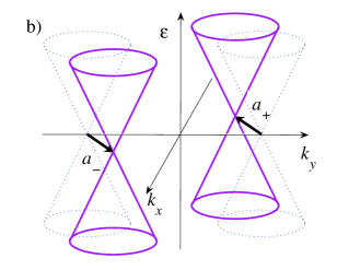
Figure 1: a) Graphene Landau level splitting, Ref.Zhang06 , attributed to spin and valley polarization. When the Zeeman energy exceeds valley anisotropy, all $N=0$ states are spin-polarized, with the $\nu=\pm 1$ states valley-polarized and the $\nu=0$ state valley-unpolarized. b) The effect of uniform strain on electron spectrum, Ref.Iordanskii85 , described by Dirac cones shift in opposite directions from the points $K$ and $K^{\prime}$. Position-dependent strain is described as a random gauge field, Eq.(2).

Can some other mechanism break pseudospin symmetry more efficiently? Coupling to disorder seems an unlikely candidate at first glance. However, there is an interesting effect that received relatively little attention, which is strain-induced random gauge field introduced by Iordanskii and Koshelev Iordanskii85 . To clarify its origin, let us consider the tight-binding model with spatially varying hopping amplitudes. Physically, such variation can be due to local strain, curvature KaneMele97 ; Morpurgo06 or chemical disorder. With hopping amplitudes $t_{i}$ for three bond orientations varying independently, we write

$$\left[\begin{array}[]{cc}0&\tau({\bf q})\\ \tau^{*}({\bf q})&0\end{array}\right]\left(\begin{array}[]{c}u\\ v\end{array}\right)=\varepsilon\left(\begin{array}[]{c}u\\ v\end{array}\right),\,\,\,\tau({\bf q})=\sum_{i=1,2,3}t_{i}e^{i{\bf q}.{\bf e}_{i}},$$ (1)

where ${\bf e}_{i}$ are vectors connecting a lattice site to its nearest neighbors, and $u$ and $v$ are wavefunction amplitudes on the two non-equivalent sublattices, $A$ and $B$. The low-energy Hamiltonian for the valleys $K$ and $K^{\prime}$ is obtained at ${\bf q}\approx\pm{\bf q}_{0}$, where $\pm{\bf q}_{0}$ are two non-equivalent Brillouin zone corners:

$$H_{\pm}=v\left[\begin{array}[]{cc}0&ip_{x}\mp p_{y}+\frac{e}{c}a_{\pm}\\ -ip_{x}\mp p_{y}+\frac{e}{c}a^{*}_{\pm}&0\end{array}\right]$$ (2)

with $a_{\pm}=\frac{c}{e}\sum_{i=1,2,3}\delta t_{i}e^{\pm i{\bf q}_{0}.{\bf e}_{i}}$, where the subscript $+(-)$ corresponds to $K(K^{\prime})$ valley. Decomposing $a_{\pm}=a_{y}\mp ia_{x}$, we see that the effective vector potential in the two valleys is given by $\pm(a_{x},a_{y})$. Notably, the field $a$ is of opposite sign for the two valleys, thus preserving time-reversal symmetry (see Fig.1b).

Here we assume that the gauge field has white noise correlations with a correlation length $\xi$,

$$\langle a_{i}(k)a_{j}(k)\rangle_{k\xi\ll 1}=\alpha^{2},\quad a_{i}(k)=\int e^{-ikr}a_{i}(r)d^{2}r,$$ (3)

as appropriate for white noise fluctuations of $\delta t_{i}$. The fluctuating effective magnetic field can be estimated as

$$\delta h(x)=\partial_{x}a_{y}-\partial_{y}a_{x}\sim\alpha/\xi^{2},$$ (4)

whereby the correlator of Fourier harmonics $\langle\delta h_{k}\delta h_{-k}\rangle$ behaves as $k^{2}$ at $k\xi\ll 1$.

Recently, strain-induced effective magnetic field was employed to explain anomalously small weak localization in graphene Morozov06 . A direct observation of graphene ripples Morozov06 yields typical corrugation length scale $\xi$ of a few tens of nanometers. Estimates from the first principles Morozov06 gave $\delta h\sim 0.1-1\,{\rm T}$, consistent with the observed degree of weak localization suppression.

Valley $K$-$K^{\prime}$ asymmetry of QHFM in the presence of the gauge field (2) translates into a uniaxial random magnetic field, proportional to (4) and aligned with the pseudospin $z$ axis. We shall see that the effect of random gauge field is subtle: somewhat counterintuitively, weak $\delta h$ induces ordering in the system, acting as an easy plane anisotropy which favors the $XY$ state. This behavior can be understood by noting that the transverse fluctuations in a ferromagnet are softer than the longitudinal fluctuations, making it beneficial for the spins to be polarized, on average, transversely to the field, as illustrated in Fig.2. This random field-induced ordering maximizes the energy gain of the spin system coupled to $\delta h$.

For magnets with uniaxial random field this behavior has been established Aharony78 ; Feldman98 in high space dimension. The situation in dimension two is considerably more delicate Pelcovits85 ; Wehr06 due to competition with the Larkin-Imry-Ma (LIM) Larkin70 ; ImryMa75 disordered state. We shall see that the anisotropy induced by random gauge field is more robust than that due to random magnetic field. (This scenario is also relevant for the two-valley QH in AlAs system Shkolnikov05 .)

The field-induced easy-plane anisotropy completely changes thermodynamics, transforming an O(3) ferromagnet, which does not order in 2d, to the XY model which exhibits a Berezinskii-Kosterlitz-Thouless transition to an ordered XY state. The transition temperature $T_{BKT}$ is logarithmically renormalized by the out-of-plane fluctuations Hikami80 , $T_{BKT}\sim{J}/{\ln(l_{XY}/\ell_{B})}$, where $l_{XY}$ is the correlation length. For fields of the order of $30\,{\rm T}$, with $l_{XY}$ given by Eq.(15) below, we obtain $T_{BKT}$ in the experimentally accessible range of a few Kelvin.

The XY-ordered QHFM state hosts fractional $\pm e/2$ charge excitations, so-called merons MacDonald95 . Merons are vortices such that in the vortex core the order parameter smoothly rotates out of the $xy$ plane. There are four types of merons MacDonald95 , since a meron can have positive or negative vorticity and the order parameter inside the core can tilt either in $+z$ or $-z$ direction. A pair of merons with the same charge and opposite vorticity is topologically equivalent to a skyrmion of charge $2(e/2)=e$ MacDonald95 .

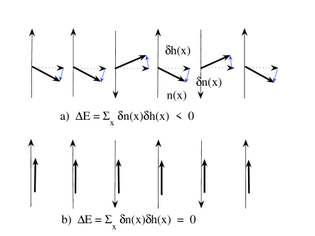
Figure 2: Random field-induced order in a ferromagnet. The energy gained from the order parameter tilting opposite to the field is maximal when the spins and the field are perpendicular (a), and minimal for the spins parallel to the field (b). Uniaxial random field induces ordering in the transverse plane.

Turning to the discussion of QH effect, the hierarchy of the spin- and valley-polarized states is determined by relative strength of the Zeeman energy and the randomness-induced anisotropy. Our estimate below obtains the anisotropy of a few Kelvin at $B\sim 30\,{\rm T}$. This is smaller than the Zeeman energy in graphene, $\Delta_{z}=g\mu_{B}B\sim 50\,{\rm K}$ at $B\sim 30\,{\rm T}$. Therefore we expect that $\nu=0$ state is spin-polarized, with both valley states filled. (This was assumed in our previous analysis Abanin06 of edge states in $\nu=0$ state.) In contrast, in highly corrugated samples, when the anisotropy exceeds the Zeeman energy, an easy-plane valley-polarized $\nu=0$ state can be favored.

While the character of $\nu=0$ state is sensitive to the anisotropy strength, the $\nu=\pm 1$ states (see Fig.1a) are always both spin- and valley-polarized. Below we focus on $\nu=\pm 1$ states, keeping in mind that for strong randomnes our discussion also applies to $\nu=0$ state.

Zeeman-split free Dirac fermion LL are given by

$$E_{n}={\rm{sgn}}(n)|2n|^{1/2}\frac{\hbar v}{\ell_{B}}\pm\Delta_{z},\quad\ell_{B}=\left(\hbar c/eB\right)^{1/2},$$ (5)

with $n$ integer and $v\approx 8\times 10^{7}\,{\rm cm/s}$. Each LL is doubly valley-degenerate. Random field (4) couples to electron orbital motion in the same way as the external field $B$, producing a local change in cyclotron energy and in the LL density. While the random field splits the $n\neq 0$ LL, for $n=0$, it does not affect the the single-particle energy (5) and couples to electron dynamics via exchange effects only. To estimate this coupling, we note that the field (4) leads to valley imbalance in exchange energy per particle:

$$E_{\rm K(K^{\prime})}=E_{\rm exch}(B\pm\delta h)=\frac{Ae^{2}}{\kappa\ell_{B\pm\delta h}},\quad A=\left(\frac{\pi}{8}\right)^{1/2},$$ (6)

where $\kappa$ is the dielectric constant of graphene.

Let us analyze the graphene QHFM energy dependence on the gauge field. We consider a fully spin- and valley-polarized $\nu=-1$ state, described by a ferromagnetic order parameter ${\bf n}=(n_{1},n_{2},n_{3})$ in the $K,K^{\prime}$ valley space. The valley-isotropic exchange interaction gives rise to a sigma model, with the gradient term only MacDonald94 :

$$E_{0}(n)=\frac{1}{2}\int J(\nabla{\bf n})^{2}d^{2}x,\quad J=\frac{e^{2}}{64\kappa\ell_{B}}.$$ (7)

The valley-asymmetric coupling to $\delta h$ in Eq.(6) generates a Zeeman-like Hamiltonian with a uniaxial random field.

$$E_{1}(n)=\int g\delta h(x)n_{3}(x)d^{2}x,\quad g=n\frac{dE_{\rm exch}}{dB}=\frac{Ane^{2}}{2B\ell_{B}},$$ (8)

where $n=1/2\pi\ell_{B}^{2}$ is the electron density.

We estimate the energy gain from the order parameter ${\bf n}(x)$ correlations with the random field, treating the anisotropy (8) perturbatively in $\delta h$. Decomposing ${\bf n}(x)=\bar{{\bf n}}+\delta{\bf n}(x)$ and taking variation in $\delta{\bf n}$, we obtain

$$J\nabla^{2}\delta{\bf n}=g\delta{\bf h}_{\perp},\quad\delta{\bf h}_{\perp}=({\bf z}-\bar{{\bf n}}(\bar{{\bf n}}\cdot{\bf z}))\delta h.$$

Substituting the solution for $\delta{\bf n}$ into the energy functional (7), (8), we find an energy gain for $\bar{{\bf n}}$ of the form

$$\delta E=-\lambda\int(1-\bar{n}^{2}_{3}(x))d^{2}x,\quad\lambda=\sum_{k}\frac{g^{2}\langle\delta h_{-k}\delta h_{k}\rangle}{2Jk^{2}},$$ (9)

where averaging over spatial fluctuations of $\delta h$ is performed. This anisotropy favors the $XY$ state, $\bar{n}_{3}=0$. Qualitatively (see Fig.2), the fluctuations due to $\delta{{\bf n}}$ tilting towards the $z$-axis minimize the energy of coupling to the uniaxial field when $\bar{{\bf n}}$ is transverse to it.

Now, let us compare the energies of the $XY$ and the Larkin-Imry-Ma state Larkin70 ; ImryMa75 . In LIM state the energy is lowered by domain formation such that the order parameter in each domain is aligned with the average field in this domain. Polarization varies smoothly between domains, and the typical domain size $L$ is determined by the balance between domain wall and magnetic field energies. In our system, the LIM energy per unit area is

$$\varepsilon_{LIM}\sim-\frac{g\Phi(L)}{L^{2}}+\frac{J}{L^{2}},$$ (10)

where $\Phi(L)$ is typical flux value through a region of size $L$. To estimate $\Phi(L)$ we write the magnetic flux through a region of size $L$ as an integral of the vector potential over the boundary, which gives

$$\Phi(L)=\oint a_{i}(x)\,dx_{i}\sim\alpha\sqrt{L/\xi}.$$ (11)

Minimizing the LIM energy (10), we find

$$\varepsilon_{LIM}\sim-\frac{g^{4}\alpha^{4}}{J^{3}\xi^{2}}.$$ (12)

Comparison to the $XY$ anisotropy $\lambda\sim-{g^{2}\alpha^{2}}/{J\xi^{2}}$ gives

$$\frac{\lambda}{\varepsilon_{LIM}}\sim\frac{J^{2}}{g^{2}\alpha^{2}}\sim\left(\frac{\Phi_{0}}{\Phi(\xi)}\right)^{2},\quad\Phi_{0}=hc/e,$$ (13)

where the flux through a region of size $\xi$ where random field does not change sign. Interestingly, the ratio (13) does not depend on the external magnetic field. Therefore, at weak randomness, when the random field flux through an area $\xi^{2}$ is much smaller than the flux quantum, the ordered $XY$ state has lower energy than the disordered LIM state.

In the opposite limit of strong randomness spins align with the local $\delta h$, forming a disordered state. It is instructive to note that for a model with white noise correlations of magnetic field, rather than of vector potential, the ratio (13) is of order one. In this case the competition of the LIM and the ordered states is more delicate.

A different perspective on the random-field-induced ordering is provided by analogy with the classical dynamics of a pendulum driven at suspension Kapitza . The latter, when driven at sufficiently high frequency, acquires a steady state with the pendulum pointing along the driving force axis. As discussed in Ref. LandauLifshitz , this phenomenon can be described by an effective potential $U_{\rm eff}$ obtained by averaging the kinetic energy over fast oscillations, with the minima of $U_{\rm eff}$ on the driving axis and maxima in the equatorial plane perpendicular to it. This behavior is robust upon replacement of periodic driving by noise noise-driven-pendulum . Our statistical-mechanical problem differs from the pendulum problem merely in that the 1d time axis is replaced by 2d position space, which is inessential for the validity of the argument. The resulting effective potential is thus identical to that for the pendulum, with the only caveate related to the sign change $U_{\rm eff}\to-U_{\rm eff}$ in the effective action, as appropriate for transtion from classical to statistical mechanics. Thus in our case the minima of $U_{\rm eff}$ are found in the equatorial plane, in agreement with the above discussion.

The easy-plane anisotropy (9) can be estimated as

$$\lambda/n\sim\frac{\delta h^{2}}{B^{2}}\times\frac{\xi^{2}}{\ell_{B}^{2}}\times\frac{e^{2}}{\kappa\ell_{B}}\approx 0.1-10\ {\rm K/particle},$$ (14)

where $\delta h\sim 0.1-1\,{\rm T}$, $\xi\sim 30\,{\rm nm}$ and $B\sim 30\,{\rm T}$ was used. Since this is smaller than the Zeeman energy, we expect that the easy-plane ferromagnet in the valley space is realized at $\nu=\pm 1$, while $\nu=0$ state is spin polarized with both valley states filled.

The out-of-plane fluctuations of the order parameter are characterized by the correlation length

$$l_{XY}\sim\sqrt{J/\lambda}\approx 1-10\,\ell_{B}$$ (15)

for the above parameter values. The length $l_{XY}$ sets a typical scale for order parameter change in the core of vortices (merons) as well as near edges of the sample and defects which induce non-zero $z$-component.

To measure the correlation length $l_{XY}$ one may use the spatial structure of $\nu=0$ wavefunction. Since the $K(K^{\prime})$ electrons reside solely on either $A$ or $B$ sublattice, the order parameter $z$-component is equal to the density imbalance between the two sublattices. The latter can be directly measured by STM imaging technique.

Finally, we briefly outline the calculation of QHFM valley anisotropy for a pure graphene sheet (the details will be published elsewhere). Let us compare the energies of state 1, in which only the valley $K$ (or $K^{\prime}$) Landau level is occupied, and state 2, with electrons in an equal-weight $K$-$K^{\prime}$ superposition state. Since the $K\,(K^{\prime})$ electrons at $\nu=0$ reside on $A\,(B)$ sublattice, the energies per particle in the Hartree-Fock approximation are given by

$$E_{1}=\frac{n}{2}\sum_{{\bf r}\in A}v_{0}V(r)\left(1-e^{-r^{2}/2l_{B}^{2}}\right),\quad V(r)=\frac{e^{2}}{\kappa r},$$

$$E_{2}=\frac{n}{4}\sum_{{\bf r}\in A,B}v_{0}V(r)\left(1-e^{-r^{2}/2l_{B}^{2}}\right),$$

where $v_{0}$ is unit cell volume. (Here we take $z=0$ to be a site of the $A$ sublattice.) We approximate the energy difference $E_{1}-E_{2}$ by the Fourier harmonic of the Hatrtree-Fock energy density at the wave vector $\left|{\bf Q}\right|\sim 1/a$, where $a\approx 0.14\,{\rm nm}$ is the graphene lattice spacing:

$$\Delta E=E_{1}-E_{2}\approx\frac{n}{4}\int V(r)\left(1-e^{-r^{2}/2l_{B}^{2}}\right)e^{i{\bf Qr}}\,d^{2}r.$$

With $Q\ell_{B}\sim\ell_{B}/a\gg 1$ at $B\simeq 30\,{\rm T}$, the integral yields

$$\Delta E\approx-\frac{27}{512\pi^{3}}\times\left(\frac{a}{l_{B}}\right)^{3}\times\frac{e^{2}}{\kappa l_{B}}\simeq 10\,{\mu}{\rm K}$$ (16)

indicating that the anisotropy is negligible.

We note that the situation is completely different for higher LL. Goerbig et al. Moessner06 pointed out that the Coulomb interaction can backscatter electrons of $K$ and $K^{\prime}$ type at LL with $n\neq 0$, which leads to a much stronger lattice anisotropy of the order $a/l_{B}$. This effect is absent for the zeroth LL due to the fact that $K$ and $K^{\prime}$ states occupy different sublattices.

In summary, we studied the valley symmetry breaking of graphene QHFM. We considered the coupling of the strain-induced random magnetic field and found that it generates an easy-plane anisotropy, which is much stronger than the symmetry-breaking terms due to lattice. The estimates of the field-induced anisotropy suggest that the random field may be a principal mechanism of $K-K^{\prime}$ QHFM symmetry breaking. The easy-plane ordered state is expected to exhibit BKT transition at experimentally accessible temperatures and half-integer charge excitations.

We are grateful to A. K. Geim, M. Kardar and P. Kim for useful discussions. This work is supported by NSF MRSEC Program (DMR 02132802), NSF-NIRT DMR-0304019 (DA, LL), and NSF grant DMR-0517222 (PAL).

References

- (1) K. S. Novoselov, A. K. Geim, S. V. Morozov, D. Jiang, Y. Zhang, S. V. Dubonos, I. V. Grigorieva, A. A. Firsov, Science, 306, 666 (2004); Proc. Natl. Acad. Sci. U.S.A., 102, 10 451 (2005).
- (2) K. S. Novoselov, A. K. Geim, S. V. Morozov, D. Jiang, M. I. Katsnelson, I. V. Grigorieva, S. V. Dubonos, A. A. Firsov, Nature 438, 197 (2005).
- (3) Y. Zhang, Y.-W. Tan, H. L. Stormer and P. Kim, Nature 438, 201 (2005).
- (4) Y. Zhang, Z. Jiang, J. P. Small, M. S. Purewal, Y. W. Tan, M. Fazlollahi, J. D. Chudow, J. A. Jaszaczak, H. L. Stormer, and P. Kim, Phys. Rev. Lett., 96, 136806 (2006).
- (5) For a review, see article by S. M. Girvin and A. H. MacDonald in Perspectives in Quantum Hall Effects, S. Das Sarma and A. Pinczuk, Eds. (Wiley, New York, 1997).
- (6) K. Yang, K. Moon, L. Zheng, A. H. MacDonald, S. M. Girvin, D. Yoshioka, and S.-C. Zhang, Phys. Rev. Lett. 72, 732 (1994).
- (7) K. Moon, H. Mori, K. Yang, S. M. Girvin, A. H. MacDonald, L. Zheng, D. Yoshioka, and S.-C. Zhang, Phys. Rev. B 51, 5138 (1995).
- (8) K. Nomura and A. H. MacDonald, Phys. Rev. Lett. 96, 256602 (2006)
- (9) M. O. Goerbig, R. Moessner and B. Douçot, cond-mat/0604554, unpublished.
- (10) J. Alicea and M. P. A. Fisher, Phys. Rev. B 74, 075422 (2006)
- (11) S. V. Iordanskii and A. E. Koshelev, ZETF Pisma, 41, 471 (1985) [translation: JETP Lett. 41, 574 (1985)].
- (12) C. L. Kane and E. J. Mele, Phys. Rev. Lett. 78, 1932 (1997).
- (13) A. Morpurgo and F. Guinea, cond-mat/0603789.
- (14) S. V. Morozov, K. S. Novoselov, M. I. Katsnelson, F. Schedin, L. A. Ponomarenko, D. Jiang, and A. K. Geim, Phys. Rev. Lett. 97, 016801 (2006).
- (15) A. Aharony, Phys. Rev. B18, 3328 (1978).
- (16) D. E. Feldman, J. Phys. A: Math. Gen. 31, 177 (1998).
- (17) B. J. Minchau and R. A. Pelcovits, Phys. Rev. B32, 3081 (1985).
- (18) J. Wehr, A. Niederberger, L. Sanchez-Palencia and M. Lewenstein, cond-mat/0604063.
- (19) A. I. Larkin, JETP 31, 784 (1970).
- (20) Y. Imry and S. K. Ma, Phys. Rev. Lett. 35, 1399 (1975).
- (21) Y. P. Shkolnikov, S. Misra, N. C. Bishop, E. P. De Poortere, and M. Shayegan, Phys. Rev. Lett. 95, 066809 (2005)
- (22) S. Hikami, T. Tsuneto, Progr. Theor. Phys. 63, 387 (1980).
- (23) D. A. Abanin, P. A. Lee and L. S. Levitov, Phys. Rev. Lett. 96, 176803 (2006).
- (24) P. L. Kapitza, Zh. Eksp. Teor. Fiz., 21, 588 (1951).
- (25) L. D. Landau and E. M. Lifshitz, Mechanics, Chap. V, §30, (Reed Educational and Pofessional Publ. Ltd, 2002)
- (26) R. L. Stratonovich and Yu. M. Romanovsky, Nauch. Dokl. Vys. Shk., ser. fiz.-mat. 3, 221 (1958) (in Russian).