Simulations for trapping reactions with subdiffusive traps and subdiffusive particles

Abstract

While there are many well-known and extensively tested results involving diffusion-limited binary reactions, reactions involving subdiffusive reactant species are far less understood. Subdiffusive motion is characterized by a mean square displacement $\langle x^{2}\rangle\sim t^{\gamma}$ with $0<\gamma<1$. Recently we calculated the asymptotic survival probability $P(t)$ of a (sub)diffusive particle ($\gamma^{\prime}$) surrounded by (sub)diffusive traps ($\gamma$) in one dimension. These are among the few known results for reactions involving species characterized by different anomalous exponents. Our results were obtained by bounding, above and below, the exact survival probability by two other probabilities that are asymptotically identical (except when $\gamma^{\prime}=1$ and $0<\gamma<2/3$). Using this approach, we were not able to estimate the time of validity of the asymptotic result, nor the way in which the survival probability approaches this regime. Toward this goal, here we present a detailed comparison of the asymptotic results with numerical simulations. In some parameter ranges the asymptotic theory describes the simulation results very well even for relatively short times. However, in other regimes more time is required for the simulation results to approach asymptotic behavior, and we arrive at situations where we are not able to reach asymptotia within our computational means. This is regrettably the case for $\gamma^{\prime}=1$ and $0<\gamma<2/3$, where we are therefore not able to prove or disprove even conjectures about the asymptotic survival probability of the particle.

1 Introduction

The survival probability of a particle diffusing in a one-dimensional medium of diffusive traps has only recently been calculated (but only asymptotically) [1, 2, 3, 4, 5]. This is surprising in view of its long history [6, 7, 8] and that of its antecedents, the so-called trapping problem [9, 10, 11, 12, 13, 14, 15, 16, 17, 18], in which the traps are static, and the target problem [15, 16, 17, 18], in which the particle does not move. The antecedent systems could be translated to tractable boundary value problems, which is not possible when both particle and traps move. The solution is an elegant “tour de force” in which the desired survival probability is bounded above and below by two others that can be posed as boundary value problems and that converge to one another asymptotically.

Recently, we undertook the generalization of the bounding approach to the case of a subdiffusive particle surrounded by a distribution of subdiffusive traps [19, 20]. Subdiffusion of a particle is usually characterized by the time dependence of the mean square of the particle displacement $x(t)$,

$$\left<x^{2}(t)\right>\sim\frac{2K_{\gamma}}{\Gamma(1+\gamma)}t^{\gamma}.$$ (1)

Here $K_{\gamma}$ is the (generalized) diffusion constant, and $\gamma$ is the exponent that characterizes normal ($\gamma=1$) or anomalous ($\gamma\neq 1$) diffusion. In particular, the process is diffusive when $\gamma=1$ and sudiffusive when $0<\gamma<1$. There are a variety of models and physical circumstances that lead to subdiffusion in the trapping and, more generally, in the binary reaction context [15, 16, 17, 21, 22, 23, 24, 25, 26, 27, 28, 29, 30, 31]. Many are based on the continuous time random walk formalism, where particles are thought of as random walkers with waiting-time distributions between steps that have broad long-time tails and consequently infinite moments, $\psi(t)\sim t^{-1-\gamma}$. Our work is based on the fractional diffusion equation, which describes the evolution of the probability density $P(x,t)$ of finding the particle at position $x$ at time $t$ by means of the fractional partial differential equation (in one dimension) [32, 33],

$$\frac{\partial}{\partial t}P(x,t)=K_{\gamma}~{}_{0}D_{t}^{1-\gamma}\frac{\partial^{2}}{\partial x^{2}}P(x,t),$$ (2)

where $K_{\gamma}$ is the generalized diffusion coefficient that appears in equation (1), and $~{}_{0}\,D_{t}^{1-\gamma}$ is the Riemann-Liouville operator,

$$~{}_{0}D_{t}^{1-\gamma}P(x,t)=\frac{1}{\Gamma(\gamma)}\frac{\partial}{\partial t}\int_{0}^{t}d\tau\frac{P(x,\tau)}{(t-\tau)^{1-\gamma}}.$$ (3)

The connection between these two approaches is in itself an interesting subject, see e.g. [34, 35].

The survival probability of a particle $A$ characterized by exponent $\gamma^{\prime}$ and generalized diffusion coefficient $K_{\gamma^{\prime}}$ surrounded by traps characterized by $\gamma$ and $K_{\gamma}$ is bounded as follows [19, 20]. An upper bound is obtained by forcing particle $A$ to remain still. The “Pascal principle” that says that the best survival strategy for the particle is to stand still was proved for the diffusive case in [8, 4, 5] and for the subdiffusive problem in our work. The solution of the fractional subdiffusion equation for the $B$ traps with the location of $A$ as an appropriate boundary then leads to the upper bound for the survival probability of $A$,

$$P_{U}(t)=\exp\left[-2\rho\frac{\sqrt{K_{\gamma}t^{\gamma}}}{\Gamma\left(1+\frac{\gamma}{2}\right)}\right],$$ (4)

where $\rho$ is the density of traps. A lower bound is calculated by allowing particle $A$ to move within a box of size ${\mathcal{L}}$ while the traps $B$ are forced to remain outside of this box. The box size is then found so as to maximize this lower bound, with the $t\to\infty$ result

$$P_{L}(t) = \frac{e^{-2}}{8\Gamma(1-\gamma^{\prime})}\left(\frac{2}{\rho}\right)^{2}\frac{1}{K^{\prime}_{\gamma^{\prime}}t^{\gamma^{\prime}}}$$ (5)

$$\times\exp\left[-2\rho\frac{\sqrt{K_{\gamma}t^{\gamma}}}{\Gamma\left(1+\frac{\gamma}{2}\right)}\right]\times\left[1+O\left(\frac{1}{\rho^{2}K^{\prime}_{\gamma^{\prime}}t^{\gamma^{\prime}}}\right)\right]$$

for $0<\gamma^{\prime}<1$. For the diffusive case ($\gamma^{\prime}=1$)

$$P_{L}(t)=\frac{4}{\pi}\exp\left[-2\rho\frac{2\sqrt{K_{\gamma}t^{\gamma}}}{\Gamma(1+\gamma/2)}-3(\pi^{2}\rho^{2}D^{\prime}t/4)^{1/3}\right].$$ (6)

With these bounds we see that for a subdiffusive particle ($0<\gamma^{\prime}<1$) and diffusive or subdiffusive traps ($0<\gamma\leq 1$) the upper and lower bounds converge asymptotically (viz., compare the logarithms of both), so that we arrive at the explicit asymptotic survival probability

$$P(t)\sim\exp\left[-2\rho\frac{\sqrt{K_{\gamma}t^{\gamma}}}{\Gamma\left(1+\frac{\gamma}{2}\right)}\right].$$ (7)

This result elicits a comment about the so-called “subordination principle” [17], according to which in some cases asymptotic anomalous diffusion behavior can be found from corresponding results for normal diffusion with the simple replacement of $t$ by $t^{\gamma}$. This can be understood from a continuous time random walk perpective because the average number of jumps made by a subdiffusive walker up to time $t$ scales as $\langle n\rangle\sim t^{\gamma}$, and in many instances the number of jumps is the relevant factor that explains the behavior of the system. However, for systems where each species has a different anomalous diffusion exponent, such a replacement becomes ambiguous. The result (7) indicates a subordination principle at work as determined by the traps. In other words, it is the motion of the traps that regulates the survival probability of the particle whether or not the particle moves, provided it does not move “too easily,” i.e., provided it is subdiffusive ($\gamma^{\prime}<1$).

When the particle is diffusive ($\gamma^{\prime}=1$) the situation is more complicated, because its asymptotic survival probability is no longer necessarily the same as it would be if it stood still. If $2/3<\gamma<1$, i.e., if the traps move sufficiently easily, the upper and lower bounds still converge and Eq. (7) still holds, that is, it is still the motion of the traps that determines the asymptotic survival probability of the particle. If the traps are subdiffusive with $\gamma=2/3$ (marginal case), the bounds lead only to a prediction of the asymptotic time dependence but not of the accompanying exponential prefactor, i.e., the bounds establish that $P(t)\sim\exp(-\lambda t^{1/3})$ but are not able to determine $\lambda$. In particular, we can not determine whether whether $\lambda$ is given by the coefficient $2\rho\sqrt{K_{2/3}}/\Gamma(4/3)$ of $t^{1/3}$ in the exponent of Eq. (7) when $\gamma=2/3$, which one might conjecture. Finally, when the particle is diffusive and the traps are sufficiently slow ($0<\gamma<2/3$), the upper and lower bounds do not have the same asymptotic time dependence, so we are not able to even functionally bound the survival probability. While it is still possible in principle that the trap-driven subordination principle continues to apply in this regime so that $\theta=\gamma/2$, we have not been able to prove or disprove such a conjecture (and the behavior at $\gamma=0$ would not fall within this conjecture, see below). If this subordination result is invalid, it would imply (and would not be surprising) that it is no longer possible to assume the particle to be standing still, and/or that it may no longer be (or only be) the exponent of the traps that regulates the motion. It is interesting to note that for $\gamma^{\prime}=1$ and $\gamma=0$, the traditional “trapping problem,” the asymptotic survival probability is [36] $P(t)\sim\exp[-3(\pi^{2}\rho^{2}D/4)^{1/3}t^{1/3}]$. One might thus be tempted to conjecture a behavior of the form $P(t)\sim\exp(-\lambda(\gamma,\rho)t^{1/3})$ throughout the range $0<\gamma\leq 2/3$, i.e., the exponential prefactor $\lambda$ would have to depend on $\gamma$ and on $\rho$. However, we have not been able to prove or disprove this conjecture either.

This analysis therefore leaves open two important questions, which we attempt to answer by way of detailed numerical simulations (although we do not entirely succeed):

1. In the cases where the bounds converge asymptotically, how much time does it take for the result to adequately describe the survival probability of the particle? In other words, how rapidly do the upper and lower bounds converge to one another?

2. Is it possible to find the asymptotic survival probability for the cases in which our analysis fails to provide converging bounds?

In part the success or failure of this attempt is of course constrained by the numerical resources at our disposal; the difficulties in numerically reaching asymptotia even in diffusion problems are well known [37].

The rest of this paper thus consists mostly of figures and a table presenting numerical simulation results. Our purpose is to ascertain the behavior of $\lambda$ and $\theta$ in the expression

$$P(t)=\exp(-\lambda t^{\theta})$$ (8)

if indeed we arrive at a regime where the survival probability exhibits this behavior. If asymptotia has been reached, we expect both to be constant with time. If they are constant, we compare their values with those obtained from the asymptotic result (7). To test $\theta$, we plot $\ln[-\ln P(t)]$ vs $\ln t$. For some cases where $\theta$ is clearly determined as a result of our simulations (i.e., constant in time and independent of $\rho$), we test $\lambda$ by plotting $-\ln P(t)/\chi$ vs $\chi$,

$$\chi\equiv\rho\langle x^{2}\rangle^{1/2}=\rho\left(\frac{2K_{\gamma}}{\Gamma(1+\gamma)}\right)^{1/2}t^{\gamma/2}.$$ (9)

$\chi$ is in effect a convenient dimensionless measure of time, and is also the ratio of the root mean square displacement of a particle at time $t$ to the average distance $\rho^{-1}$ between traps.

In section 2 we briefly outline our simulation methodology. Section 3 is a compendium of our results, along with the associated descriptions. A recapitulation is presented in section 4.

2 Numerical simulation methodology

A brief review of our numerical simulation methodology is appropriate at this point. We generate the trap distribution by placing a trap at each site of a one-dimensional lattice with probability $\rho$ (and not placing a trap with probability $1-\rho$). The particle $A$ is placed at the origin of the lattice. The typical lattice has $10\,000$ sites, and we implement periodic boundary conditions. We have simulated larger lattices and different (free) boundary conditions to ascertain that the results are not affected.

The dynamics of a moving particle in a sea of moving traps is implemented as follows. Each particle and trap is assigned an “internal clock” starting at time $t=0$ according to their waiting time probability distributions. One particular trap, or the particle, will be the first to take a step, left or right with equal probability ($1/2$). We check if trapping of the particle occurs as a result. If it does, we stop the dynamics, record the time, and generate a new ensemble of traps plus one particle. If it does not, we continue the dynamics by observing the very next trap or particle that takes a step. Again, if trapping occurs, the time is recorded and the dynamics stopped; if not, the walk continues. We also define a maximal time threshold (dictated by our computational resources) at which we stop the dynamics.

In order to collect enough statistics we have run a large number of realizations (ensembles of traps and particle) of the dynamics, typically on the order of $50\,000$. A $64$-bit congruential random number generator was used througout the program [38]. The output of interest of each realization is the time when the particle is annhilated. On the basis of this observable we construct the integrated probability distribution of particle survival. The statistical errors have been computed using the jackknife procedure [39].

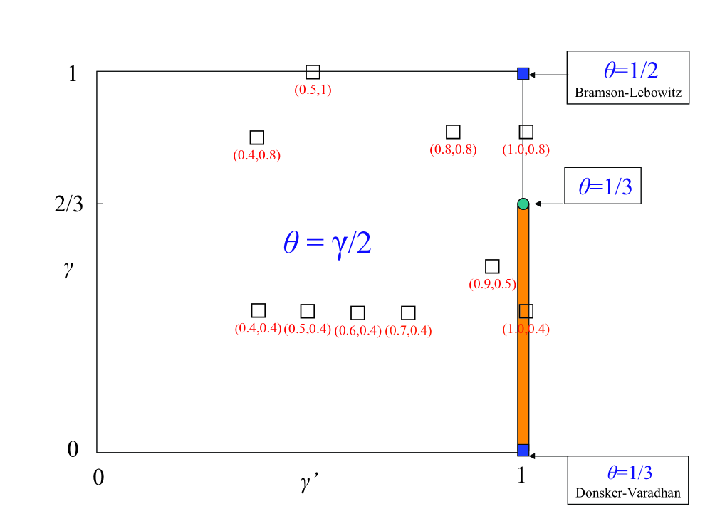
Figure 1: $\gamma$-$\gamma^{\prime}$ parameter space indicating regions of analytic asymptotic predictions for the exponent $\theta$ and the coefficient $\lambda$ in $P(t)\sim\exp(-\lambda t^{\theta})$. No predictions are available along the thick strip (orange in colour version) $\gamma^{\prime}=1$, $0<\gamma<2/3$. The exponent is predicted at the end points of the thick strip, the prefactor only at the lower end point.

3 Results

We will see that our numerical simulations of the problem $A+B\to B$ when both the traps $B$ and the particle $A$ are mobile approach asymptotic behavior far more rapidly in some regions of parameter space than in others. Figure 1 shows a $\gamma$-$\gamma^{\prime}$ space in which are indicated regions and points of exponents $\theta$ predicted analytically. The thick (orange in colour rendition) strip on the right (not including its end points) represents the parameter regime where the upper and lower survival probability bounds do not coverge asymptotically and hence no predictions (aside from conjectures) have been made. The prefactor $\lambda$ has also been predicted everywhere except on the thick (orange) strip and its upper end point, indicated by a circle (green in colour rendition). The empty squares in figure 1 indicate the pairs ($\gamma^{\prime},\gamma$) where we have carried out numerical simulations. All of our results for the apparent exponent $\theta$ obtained from the simulations for these points are summarized in table 1, and a number of them are subsequently exhibited in figures.

Table 1: Numerical simulation results for the apparent exponent $\theta$ in the survival probability of the particle $A$. The first five sets of results are for the parameter regime $\gamma<\gamma^{\prime}$. The next four sets are for $\gamma\geq\gamma^{\prime}$. Only the last set is in the regime $0<\gamma<2/3$, $\gamma^{\prime}=1$ for which we have no bounding results. In addition we show the $\chi^{2}/\mathrm{d.o.f}$ of the fit - $\mathrm{d.o.f}$ being the number of degrees of freedom of the fit-, the number of realizations performed, $N_{R}$, and the logarithm of the minimum value of time used on each fit, $\ln(t_{\mathrm{min}}^{\mathrm{fit}})$. The statistical error in $\theta$ (one standard deviation) has been computed using a jackknife procedure.

• Traps($\gamma$)	Particle($\gamma^{\prime}$)	$\rho$	$\theta$	$\gamma/2$	$\ln(t_{\mathrm{min}}^{\mathrm{fit}})$	$\chi^{2}/\mathrm{d.o.f}$	$N_{R}$
  		$\gamma<\gamma^{\prime}$
  $0.4$	$0.5$	$0.01$	$0.146(7)$	$0.2$	$27.2$	$0.58$	460000
  		$0.1$	$0.175(3)$	$0.2$	14.47	0.37	511733
  $0.4$	$0.6$	$0.01$	$0.121(4)$	$0.2$	25.12	0.26	2050560
  		$0.1$	$0.155(4)$	$0.2$	15.74	1.05	1398048
  $0.4$	$0.7$	$0.1$	$0.093(5)$	$0.2$	24.8	0.81	6908894
  		$0.5$	$0.190(4)$	$0.2$	8.17	1.04	2106963
  $0.5$	$0.9$	$0.01$	$0.124(2)$	$0.25$	18.5	0.6	38523723
  		$0.1$	$0.176(4)$	$0.25$	11.9	1.08	2285460
  		$0.5$	$0.262(6)$	$0.25$	6.25	0.93	789940
  $0.8$	$1.0$	$0.01$	$0.423(2)$	$0.4$	12	1.00	13626177
  		$0.1$	$0.430(5)$	$0.4$	3.55	0.83	618793
  		$\gamma\geq\gamma^{\prime}$
  $0.4$	$0.4$	$0.1$	$0.186(2)$	$0.2$	15.2	0.43	548122
  		$0.5$	$0.210(2)$	$0.2$	6.47	1.05	425840
  $0.8$	$0.4$	$0.01$	$0.396(4)$	$0.4$	11.5	0.4	111208
  		$0.1$	$0.378(2)$	$0.4$	5.58	0.7	225796
  $0.8$	$0.8$	$0.01$	$0.374(2)$	$0.4$	12.14	1.03	325275
  		$0.1$	$0.361(3)$	$0.4$	8.64	1.03	618793
  $1.0$	$0.5$	$0.01$	$0.501(2)$	$0.5$	7.5	0.5	3159970
  		$0<\gamma<2/3,~{}\gamma^{\prime}=1$
  $0.4$	$1.0$	$0.01$	$0.427(6)$	$0.2$	10	1.06	11952
  		$0.1$	$0.433(7)$	$0.2$	5	1.05	7740
  		$0.5$	$0.474(7)$	$0.2$	3	1.0	10000

The table leads to a number of broad conclusions, starting with the assertion that in the parameter regime $\gamma\geq\gamma^{\prime}$ we have been able to reach the asymptotic exponent $\theta$, and that this exponent agrees with the theoretical asymptotic prediction. In this regime the slope we identify as $\theta$ is indeed insensitive to trap density changes and close to the asymptotic value $\gamma/2$. We have listed four sets of results for $\gamma\geq\gamma^{\prime}$, and exhibit three of them explicitly in figures 2, 3, and 4. We see that the time to achieve asymptotic behavior increases drastically with decreasing $\gamma$ for a given $\rho$. For example, for the same $\rho$ in figures 2 and 3, we need to go to $\ln(t)>20$ or so for $\gamma=0.4$ but only to $\ln(t)>10$ or so for $\gamma=0.8$. For a given pair of parameters $(\gamma,~{}\gamma^{\prime})$, the time needed to reach asymptotic behavior is of course greater when the density of traps is lower. Note also that this time seems insensitive to the value of $\gamma^{\prime}$: for the case in the table not shown in a figure ($\gamma=\gamma^{\prime}=0.8$), the abscissa $\ln(t)$ covers the same range for the same trap densities as those in figure 3.

Figure 2: Simulation results for $\gamma=\gamma^{\prime}=0.4$. The left set of data (black in colour version) corresponds to a trap density $\rho=0.5$ and a slope of $0.210$; the right set (red in the colour version) to $\rho=0.1$ and a slope of $0.186$. The asymptotic prediction for the slope is $\gamma/2=0.2$. The error bars of the points are smaller than the size of the symbols (the same in figures  3 to 8).

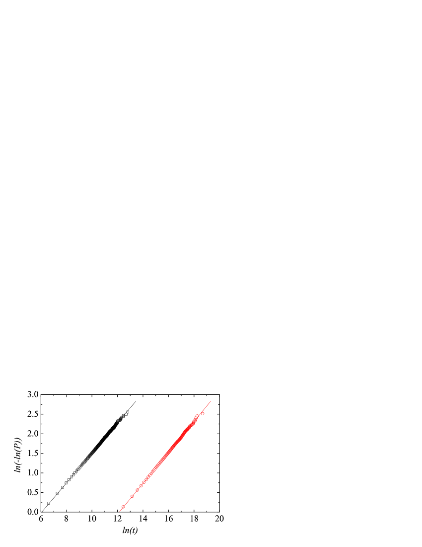
Figure 3: Simulation results for $\gamma=0.8$ and $\gamma^{\prime}=0.4$. The left set of data (black) corresponds to a trap density $\rho=0.1$ and a slope of $0.378$; the right set (red) to $\rho=0.01$ and a slope of $0.396$. The asymptotic prediction for the slope is $\gamma/2=0.4$.

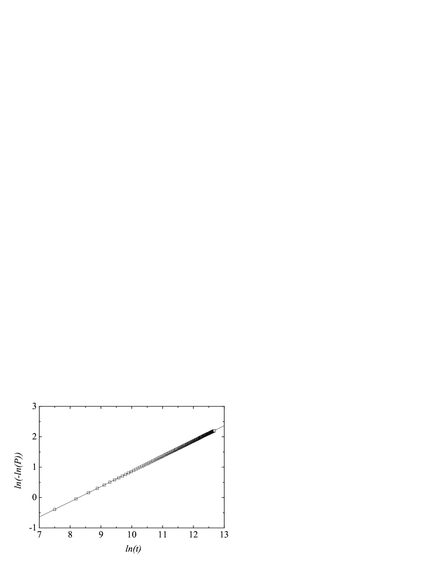
Figure 4: Simulation results for $\gamma=1$ and $\gamma^{\prime}=0.5$. Only one set of data points is shown, for $\rho=0.01$. The slope is $0.501$. The asymptotic prediction for the slope is $\gamma/2=0.5$.

The situation is more complicated and less satisfactory for $\gamma<\gamma^{\prime}$. This is seen into the first five sets of results in table 1. Although (as we will see in the figures) a clear slope can be read off the simulation data for $\ln[-\ln P(t)]$, this slope is not independent of $\rho$ in most cases, nor does it yet satisfactorily approach the theoretically predicted asymptotic value. We conclude that in this parameter regime asymptotia requires a much longer time than we can reasonably simulate, that is, when the particle moves “more easily” than the traps, it takes the system a much longer time to behave as it would if the particle were simply sitting still. Nevertheless, within this range of parameters there are some statements of “quality” than can be made, as shown in figures 5, 6, and 7. The most salient point seems to be that asymptotia is reached more readily when both $\gamma$ and $\gamma^{\prime}$ are closer to the diffusive case and closer to one another. Thus the results in figure 7 are satisfactory (i.e., essentially independent of $\rho$ and in fair agreement with the asymptotic slope) within a reasonable time range. If $\gamma^{\prime}$ is close to unity but $\gamma$ is too small, it is clearly difficult to reach asymptotia, as evidenced in the results of figure 6. If both $\gamma$ and $\gamma^{\prime}$ are small then even going to extraordinarily long times as shown in figure 5 is not sufficient.

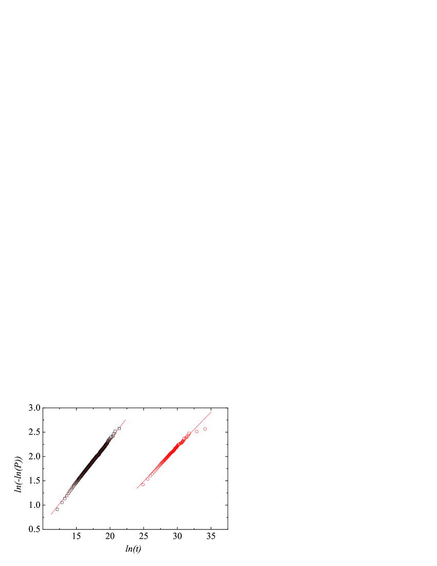
Figure 5: Simulation results for $\gamma=0.4$ and $\gamma^{\prime}=0.5$. The left set of data (black in colour version) corresponds to a trap density $\rho=0.1$ and a slope of $0.175$; the right set (red in the colour version) to $\rho=0.01$ and a slope of $0.146$. The asymptotic prediction for the slope is $\gamma/2=0.2$.

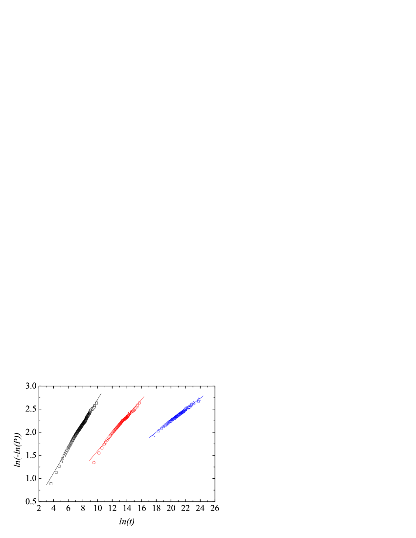
Figure 6: Simulation results for $\gamma=0.5$ and $\gamma^{\prime}=0.9$. The left set of data (black) corresponds to a trap density $\rho=0.5$ and a slope of $0.262$; the middle set (red) to $\rho=0.1$ and a slope of $0.176$; the right set (blue) to $\rho=0.01$ and a slope of $0.124$. The asymptotic prediction for the slope is $\gamma/2=0.25$.

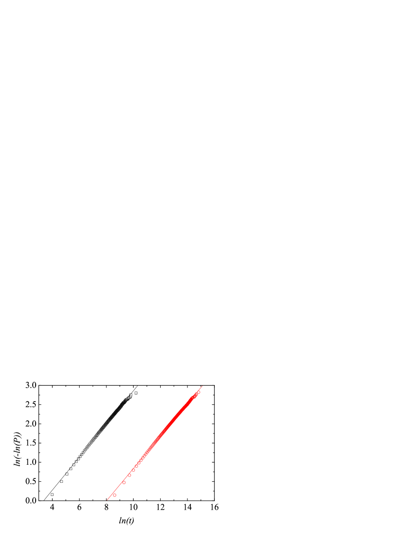
Figure 7: Simulation results for $\gamma=0.8$ and $\gamma^{\prime}=1$. The left set of data (black) corresponds to a trap density $\rho=0.1$ and a slope of $0.430$; the right set (red) to $\rho=0.01$ and a slope of $0.421$. The asymptotic prediction for the slope is $\gamma/2=0.4$.

Finally, it is apparent that the simulation results for the “problem case” $0<\gamma<2/3$, $\gamma^{\prime}=1$ lead to a slope that seems well defined (see figure 8) and relatively insensitive to $\rho$. It is therefore tempting to relate this slope to asymptotic behavior. However, the value of the slope does not confirm either of the conjectures put forther earlier, namely, that it is perhaps equal to $\gamma/2$ or to $1/3$. The slope is not particularly close to either of these values. On the other hand, the observation does not necessarily disprove the conjectures, since it is not clear that asymptotia has been reached. In fact, the observed slope is closer to that expected for the short-time behavior of a normally diffusing particle surrounded by stationary traps, $\theta=1/2$. Thus the question of the asymptotic behavior in this regime is still open.

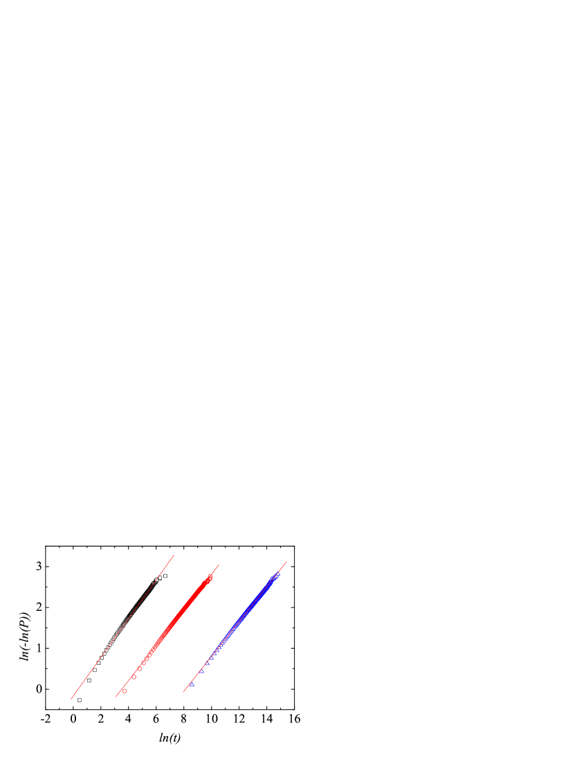
Figure 8: Simulation results for $\gamma=0.4$ and $\gamma^{\prime}=1$. The left set of data (black) corresponds to a trap density $\rho=0.5$ and a slope of $0.474$; the middle set (red) to $\rho=0.1$ and a slope of $0.433$; the right set (blue) to $\rho=0.01$ and a slope of $0.427$. There is no asymptotic prediction for the slope in this regime, but two conjectures would be that it might be $1/3$ or $\gamma/2=0.2$.

We have thus found up to this point that our numerical simulations are able to confirm the asymptotic prediction for the survival probability of a particle $A$ characterized by (sub)diffusion exponent $\gamma^{\prime}$ surrounded by traps $B$ characterized by exponent $\gamma$ provided that $\gamma<\gamma^{\prime}$, but that it is difficult to do so for $\gamma\geq\gamma^{\prime}$. For the regime $0<\gamma<2/3,~{}\gamma^{\prime}=1$ we have no asymptotic theory, and the numerical results do not inform us about the validity of conjectured behaviors.

Having determined the exponent $\theta$ in the survival probability expression (8) in some parameter regimes, it remains to explore whether we can numerically determine, or at least bound, the exponential prefactor $\lambda$. This turns out to be difficult. In figure 9 we show our simulation results for the case $\gamma=\gamma^{\prime}=0.4$ of figure 2. We also show the upper bound, which is exactly the asymptotic prediction, cf. compare equations (4) and (7), and so appears as a straight (broken) line in the figure. It lies in the lower part of the figure because of the minus sign in the ordinate. The lower bound of equation (5), which only approaches the upper bound asymptotically, is shown as the dotted curve. The simulation results are for $\rho=0.1$ and $\rho=0.5$, and fall between the bounds. However, we would have to go to times far longer than we are able to in order to ascertain the asymptotic prediction. A similar figure, but for only one concentration, $\rho=0.01$, is shown in figure 10 for $\gamma=1$ and $\gamma^{\prime}=0.5$. Here the upper and lower bounds do not even find their rightful relative placements until a time far beyond our simulation capabilities, although the simulation results at least point in the right direction. It is, in any case, clearly very difficult to determine the prefactor $\lambda$ and even to ascertain that it is properly bounded by the theory.

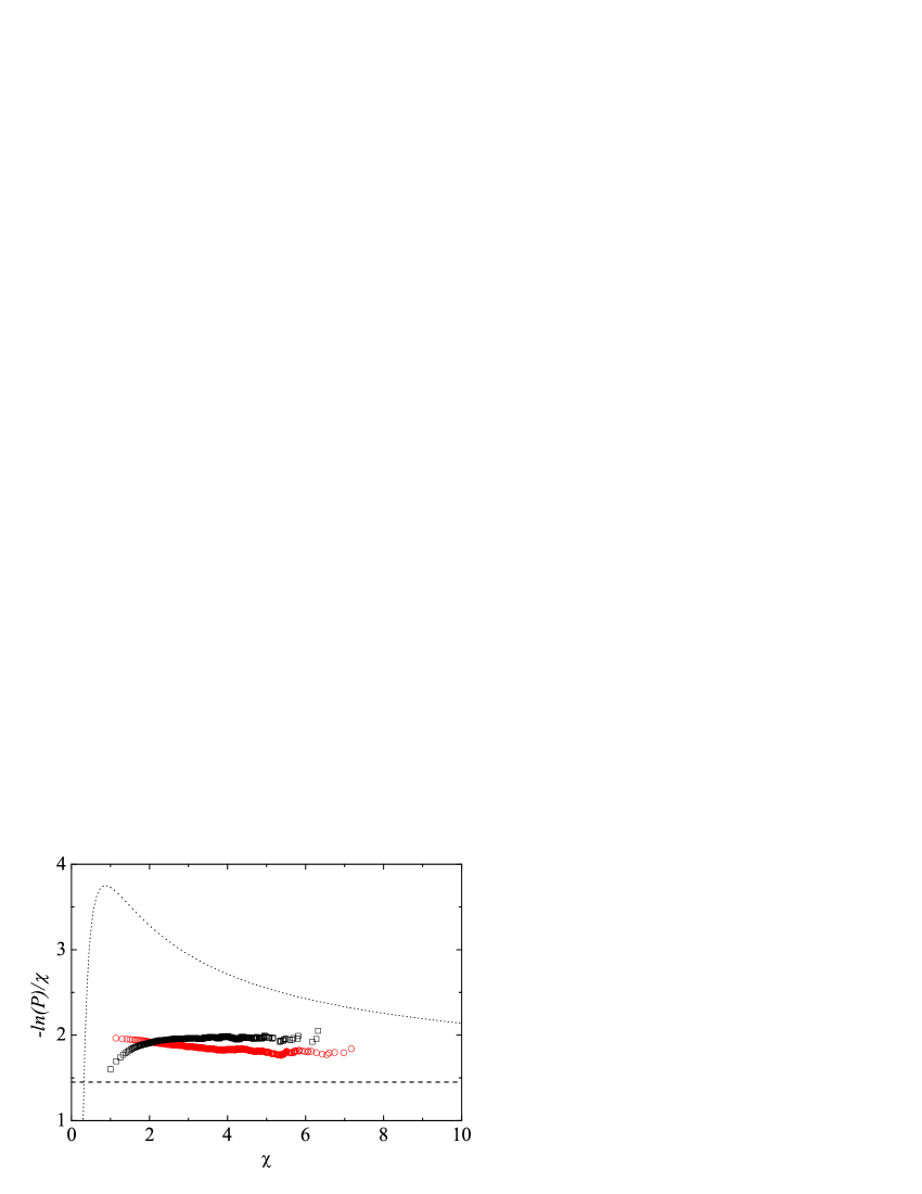
Figure 9: Simulation results for the exponential prefactor $\lambda$ in equation (8) for $\gamma=\gamma^{\prime}=0.4$. Broken line: upper bound; Dotted curve: lower bound. Data points are for $\rho=0.1$ (red, lower set) and $\rho=0.5$ (black, upper set).

Figure 10: Simulation results for the exponential prefactor $\lambda$ in equation (8) for $\gamma=1$ and $\gamma^{\prime}=0.5$. Broken line: upper bound; Dotted curve: lower bound. Data points are for $\rho=0.01$.

4 Recap

In this paper we have made an attempt to assess the validity of the asymptotic predictions for the survival probability of a (sub)diffusive particle $A$ characterized by exponent $\gamma^{\prime}$ surrounded by (sub)diffusive traps of density $\rho$ characterized by exponent $\gamma$. The prediction is arrived at by obtaining an upper and a lower bound to the survival probability that in most parameter regimes converge to one another [19, 20]. This asymptotic survival probability in fact turns out to be exactly the upper bound, which is calculated under the assumption that particle $A$ remains still. It is thus the case that in the parameter regime where this prediction is valid it eventually makes no difference whether or not particle $A$ moves; the asymptotic survival probability is entirle determined by the motion of the traps. However, when $\gamma^{\prime}=1$ and the traps are “too slow” ($0<\gamma<2/3$), the bounds no longer converge even asymptotically, and this approach does not lead to a prediction. In other words, it is no longer evident that the motion of the particle does not matter. We have proposed two conjectures for this regime. One is that in fact the motion of the particle does not matter, as before, but our numerical results do not seem to support this assumption. The other relies on the fact that for a diffusive particle we know something about the asymptotic survival probability at the two extreme points of this interval, namely at $\gamma=0$ (when the traps are stationary) and at $\gamma=2/3$. In both of these cases the survival probability decays as $P(t)\sim\exp\left(-\lambda t^{1/3}\right)$ (with $\lambda$ known for the former but not for the latter), and so one might conjecture a $t^{1/3}$ dependence in the unknown range. However, this conjecture could not be verified either.

In the regimes where there is an asymptotic prediction, we are able to verify it quite clearly when $\gamma\geq\gamma^{\prime}$, that is, when the particle moves more slowly or at the same pace than the traps. Again, the results indicate that the particle could just as well sit still to reach the same asymptotic survival probability as it does when it moves. Also, the “time to asymptotia” is insensitive to the value of $\gamma^{\prime}$, but it is shorter when $\gamma$ is larger and when the density of traps is higher. We also tested our ability to predict the asymptotic exponential prefactor $\lambda$, but find that at best we can show that it lies between the correct bounds. At worst, the bounds do not take their rightful places until times that we can not reach with our simulations.

When $\gamma<\gamma^{\prime}$ the situation is far more difficult, increasingly so with increasing difference between the two exponents. It would seem to be necessary to go beyond the leading asymptotic term to thoroughly understand the dynamics for these cases. This has been done with some measure of success in the purely diffusive problem [40].

Our simulation method can not be stretched beyond the times implemented in this work. We have been able to answer some questions and ascertain some predictions, but not others. To reach the longer times needed to deal with the questions that we have not been able answer conclusively will require new simulation optimization methods. Such methods have been developed for diffusive particles and traps [37], but their generalization to the subdiffusive problem does not appear evident.

References

References

- [1] Bray A J and Blythe R A 2002 Phys. Rev. Lett. 89 150601
- [2] Blythe R A and Bray A J 2003 Phys. Rev. E 67 041101
- [3] Oshanin B, Bénichou O, Coppey M and Moreau M 2002 Phys. Rev. E 66 060101R
- [4] Moreau M, Oshanin G, Bénichou O and Coppey M 2003 Phys. Rev. E 67 045104R
- [5] Bray A J, Majumdar S N and Blythe R A 2003 Phys. Rev. E 67 060102
- [6] Bramson M and Lebowitz J L 1988 Phys. Rev. Lett. 61 2397
- [7] Bramson M and Lebowitz J L 1991 J. Stat. Phys. 62 297
- [8] Burlatsky S F, Oshanin G S and Ovchinnikov A A 1989 Phys. Lett. A 139 241
- [9] Hughes B F 1995 Random Walks and Random Environments, Volume 1: Random Walks (Oxford: Clarendon Press)
- [10] Hughes B F 1996 Random Walks and Random Environments, Volume 2: Random Environments (Oxford: Clarendon Press)
- [11] Weiss G H 1994 Aspects and Applications of the Random Walk (Amsterdam: North-Holland)
- [12] den Hollander F and Weiss G H 1994 in Contemporary Problems in Statistical Physics ed G H Weiss (Philadelphia: SIAM) p 147
- [13] Havlin S and ben Avraham D 1987 Adv. Phys. 36 695
- [14] ben Avraham D and Havlin S 2000 Diffusion and Reactions in Fractals and Disordered Systems (Cambridge: Cambridge University Press)
- [15] Zumofen G, Klafter J and Blumen A 1983 J. Chem. Phys. 79 5131
- [16] Klafter J, Blumen A and Zumofen G 1984 J. Stat. Phys. 36 561
- [17] Blumen A, Klafter J and Zumofen G 1986 in Optical Spectroscopy of Glasses ed I Zschokke (Dordrecht: Reidel).
- [18] Redner S 2001 A Guide to First-Passage Processes (Cambridge: Cambridge University Press)
- [19] Yuste S B and Lindenberg K 2005 Proc. SPIE 5845 27
- [20] Yuste S B and Lindenberg K 2005 Phys. Rev. E 72 061103
- [21] Sung J and Silbey R J 2003 Phys. Rev. Lett. 91 160601
- [22] Seki K, Wojcik M and Tachiya M 2003 J. Chem. Phys. 119 2165
- [23] Henry B I and Wearne S L 2000 Physica A 276 448
- [24] Henry B I and Wearne S L 2002 SIAM J. Appl. Math. 62 870
- [25] Vlad M O and Ross J 2002 Phys. Rev. E 66 061908
- [26] Fedotov S and Méndez V 2002 Phys. Rev. E 66 030102
- [27] Sung J, Barkai E, Silbey R J and Lee S 2002 J. Chem. Phys. 116 2338
- [28] Yuste S B and Acedo L 2004 Physica A 336 334
- [29] Yuste S B and Lindenberg K 2001 Phys. Rev. Lett. 87 118301
- [30] Yuste S B and Lindenberg K 2002 Chem. Phys. 284 169
- [31] Yuste S B, Acedo L and Lindenberg K 2004 Phys. Rev. E 69 036126
- [32] Metzler R and Klafter J 2000 Physica A 278 107
- [33] Schneider W R and Wyss W 1989 J. Math. Phys. 30 134
- [34] Barkai E 2003 Phys. Rev. Lett. 90 104101
- [35] Mainardi F, Vivoli A and Gorenflo R 2005 Fluct. and Noise Lett. 5 L291
- [36] Donsker M D and Varadhan S R S 1975 Comm. Pure Appl. Math. 28 525
- [37] Mehra V and Grassberger P 2002 Phys. Rev. E 65 050101
- [38] Ossola G and Sokal A D Nucl. Phys. B 691 259
- [39] Efron B 1982 The Jackknife, the Bootstrap and other Resampling Plans (Philadelphia: SIAM)
- [40] Anton L and Bray A J 2004 J. Phys. A 37 8407